Journal of
Applied Research on Industrial Engineering
Journal of Applied Research on Industrial Engineering Vol. 1, No. 4 (2014) 208-229
Proposing Objective Mathematical Model for Design of
Multi-Product Forward and Reverse Logistics Network
Ehsan Hashemi
1*1, Reza Tavakkoli-Moghaddam
22, Mahdi Bashiri
31Department of Industrial Engineering, Najafabad Branch, Islamic Azad University, Isfahan, Iran ([email protected]) 2 Department of Industrial Engineering, University of Tehran, Tehran, Iran ([email protected])
3Department of Industrial Engineering, Shahed University, Tehran, Iran, Iran ([email protected])
A B S T R A C T A R T I C L E I N F O
The attestation towards environmental, statutory obligations and economic interests arising from rehabilitation operations in recent years has led to more focus on reverse logistics operations. To this end, integration of the design of reverse and forward logistics networks which results in prevention of sub optimality due to separated design of these networks is of high significance. This model discusses a mixed-integer nonlinear programming model for the integrated design of multi-level and multi-commodity forward-reverse supply chain network. In the end, the calculation results of the proposed model solution have been presented via GAMS software in order to locate facilities, determine the relationship between facilities and raw material procurement rate and production rate. The result of the solved multi-purpose models has corroborated the single-purpose models and it shows the efficiency of the used methods.
Article history : Received: 19 September 2014 Received in revised format: 20 October 2014
Accepted: 25 October 2014 Available online: 1 December 2014
Keywords :
Closed-Loop Logistics, Mixed Integer Nonlinear Programming,
Multi-Product, Multi-Objective
1.
Introduction
Since the relationship of raw materials and product in the opponent direction to supply chain is an inevitable issue due to various reasons, it is necessary to design a reverse logistics network. Various definitions have been suggested for the reverse logistics. "Reverse logistics is the efficient and effective process of planning, implementing and controlling of inputs as well as storing of second-hand commodities and their relevant data with the purpose of either value recovery or proper disposal in opponent direction to the traditional supply chain" (Fleischmann
209
et al., 2001).Products and materials are returned due to different reasons: impaired products that may be repaired once again, products in the final stage of their lifecycles that still have value, unsold and unwanted products on retailers' shelves, returned products, wastes and dangerous substances (Bernon and Cullen, 2007). Moreover, products at the end of their lease or warranty periods and the damaged ones are considered as returned products. In case these returned products are not managed and controlled efficiently, then the manufacturers of main equipment would sustain more costs (Pishvaee et al., 2009).
Execution of strategic decisions calls for spending of huge sums as it would be costly to apply changes following the establishment of factories and distribution centers. Hence, strategic decisions must be adopted such that they are least deviated from optimum state through time. The choice of objective and identification of existing and future circumstances would have a great contribution to adoption of better strategic decisions. The main objective here is to minimize the costs of network (Santoso et al., 2005). Minimization of time delays and deterioration products are of those targets less discussed by the researchers.
Most of the previous studies have considered the design of forward and reverse logistics networks separately but configuration of reverse logistics network influences the forward logistics network to a great extent. Separate design may lead to sub optimality. Therefore, the design of the forward and reverse logistics network must be integrated which entails more efforts to be made in order to simultaneously analyze both forward and reverse logistics networks (Lee and Dong, 2008). Network design is also considered an important strategic decision in the supply chain. Generally speaking, the design of logistics network includes the determination of number, location and capacity of facilities and the relationship between facilities. Moreover, the existing literatures suggest that a major part of relevant articles in the past had been focused on the design of single-purpose network which mostly consists of cost reduction and only a few research conducted in recent years have taken on the subject of design of multi-objective reverse logistics network and that is while the decision makers in designing of real networks often tend to optimize more than one objective (Amiri, 2006).
This article proposes a model for design of multi-product integrated logistics network with restricted capacity. The output of this model is the detection of facilities and relationship between facilities, determination of costs, production rates, amount of procured raw materials and the unsatisfied demand. The objectives of this model include minimization of costs, time delays and number of deterioration products and row materials.
2.
Literature Review
210
layers of repair, collection, manufacturer and customer was design by Eskandarpour et al. (2013) to develop a post-sale service network.
In their single-period and multi-product article, Ramezani et al. (2013) considered the maximum revenue and response to customer and the quality of raw materials as the objectives of model while supplier, manufacturer and distributor layers are considered in the forward path and collection, reproduction and disposal centers are considered in the reverse path. Tabrizi and Razmi (2013), designed a mixed-integer nonlinear mathematical model in their article. Fuzzy set theory was used to determine uncertainty and Benders decomposition method was used to solve the model. Amin and Zhang (2013) designed a model aimed at minimization of costs for the closed-loop supply chain network and then developed a bi-objective model by considering uncertainty in demand and returned products.
Keyvanshokooh et al. (2013) applied a dynamic pricing approach for the returned products in addition to design of a multi-period and multi-product integrated supply chain network. The returned products in this model are classified based on the level of their qualities and a different procurement price is provided for each class. Hatefi and Jolai (2013) considered a single-period multi-product model with production and distribution centers in the forward path and the collection, recycling and disposal centers in the reverse path. The purpose of this model is to minimize the costs. Tafti et al. (2014) designed an integrated form of supply chain network. Their proposed network included assembly, customers, collection, and disposal centers. Demand and cost parameters in this multi-period model were considered as uncertain and fuzzy. Pishvaee et al. (2014) using a multi-objective programming model designed a supply chain network for pharmaceutical industry. The proposed model was a solid one consisting of economic, environmental and social targets. A multi-objective and multi-product model was proposed by Ramezani et al. (2014) in order to develop a closed-loop supply chain network in fuzzy environment. The relocation of products between the two levels is facilitated through transportation. The proposed model consists of four layers in forward path (supplier, manufacturing, distribution and customers) and three layers in reverse path (customers, collection and disposal centers). The objectives of this model include maximization of revenue, service level and sigma quality level. Ozceylan et al. (2014) have simultaneously taken into account both tactical and strategic decisions in their model such that the issues related to development of supply chain network and logistics are considered in the strategic phase while the tactical phase is related to balance of assembly lines.
In the single-product model of Hatefi et al. (2014), production and reproduction centers as well as distribution and collection centers are considered modular and parameters of demand and product return rate, shipment and operational costs, facilities capacity are considered as fuzzy and the objective function comprises the minimization of costs. Demirel et al. (2014) developed a multi-period mixed linear programming model for closed-loop supply chain network. The pricing in secondary market and encouraging policies have been considered. The capacity of all facilities in this model is restricted and demand is certain with no allowable shortages. Presenting a systematic approach, Vahdani et al (2014) developed a reliable network of facilities in the closed-loop supply chain network in uncertain circumstances. A case study of an iron factory was considered in this model so that the results would become much closer to the real world.
211
responsible to manage inventory in DCs and deliver products to customers. Furthermore, they proposed a non-dominated sorting genetic algorithm to perform high-quality search using two-parallel neighborhood search procedures for creating initial solutions. The potential of this algorithm has been evaluated by its application to the numerical example. Then, the obtained results have been analyzed and compared with multi-objective simulated annealing. Ghorbani et al. (2014) considered a fuzzy goal programming approach for solving a multi-objective model of reverse supply chain design. This model involves of three objectives that they minimize recycling cost, rate of waste generated by recyclers and material recovery time in such a way that the best set of recyclers to allocate products is determined. The main contribution of the proposed model is that it considers cost, time and efficiency rate to design responsive and efficient reverse supply chain.
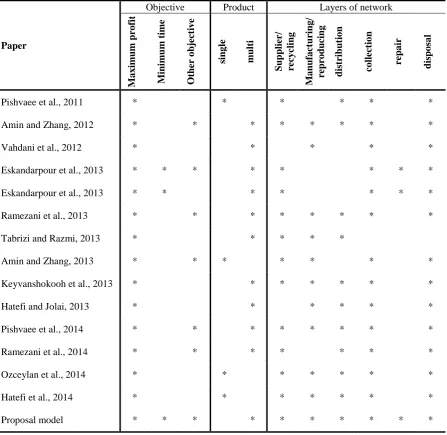
Table 1 Review of some existing models.
Paper
Objective Product Layers of network
M
a
x
imu
m
pro
fit
M
ini
mu
m t
ime
O
ther
o
bje
ct
iv
e
sing
le
mu
lt
i
Su
pp
lier/
re
cy
cling
M
a
nu
fa
ct
uring
/
re
pro
du
cing
dis
trib
utio
n
co
llect
io
n
re
pa
ir
dis
po
sa
l
Pishvaee et al., 2011 * * * * * *
Amin and Zhang, 2012 * * * * * * * *
Vahdani et al., 2012 * * * * *
Eskandarpour et al., 2013 * * * * * * * *
Eskandarpour et al., 2013 * * * * * * *
Ramezani et al., 2013 * * * * * * * *
Tabrizi and Razmi, 2013 * * * * *
Amin and Zhang, 2013 * * * * * * *
Keyvanshokooh et al., 2013 * * * * * * *
Hatefi and Jolai, 2013 * * * * * *
Pishvaee et al., 2014 * * * * * * * *
Ramezani et al., 2014 * * * * * * *
Ozceylan et al., 2014 * * * * * * *
Hatefi et al., 2014 * * * * * * *
Proposal model * * * * * * * * * *
212
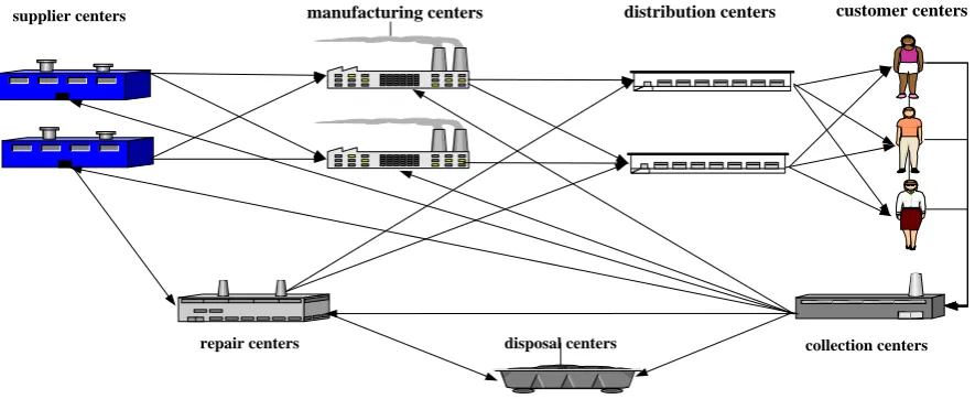
Also, most of the articles have only considered either of repair, recycling, reproduction or redistribution. Therefore, in the multi-product closed-loop logistics network model of this article, the layers of supplier, manufacturer and distributer are considered for the forward path while the reverse path includes the layers of recycling, reproduction, repair and disposal. The deterioration rate has been considered in the proposed model for production rate and procured raw materials. Various modes of transportation have been considered in the relationships of facilities. Moreover, the not estimated demand rate and the minimum number of transportation means between distribution and customer are considered as the output variable. One of the innovations of this model is that some of the products dispatched to the repair centers undergo part replacements with the replaced parts dispatched to disposal and supplier centers and the repaired product would be returned to distribution centers once the parts have been replaced. The quality of repaired products have been considered equivalent to that of new products.
3.
Problem definition
213
supplier centers manufacturing centers distribution centers customer centers
disposal centers collection centers repair centers
Fig 1 Structure of Integrated Forward/Reverse Logistics Network
Accordingly, the problem of designing a logistics network is defined as an allocation-location single-period, multilayered, multi-product capacitated facilitation and the number of factories, distribution, collection, repair and waste disposal centers, their levels of capacity and the relationship of facilities will be provided in order to select and determine the location.
4.
Model assumptions and limitation
The problem of integrated multi-product and multi-level logistics has been modeled and planned with respect to the following assumptions:
Locations of customers and suppliers are pre-specified and constant.
The reverse flow is compressive and comes as a percentage of demand in forward
mode.
The model is planned and simulated based on a certain period.
Each collection and distribution center may cover customers within a specified range.
5.
Model formulation
The parameters used in the mathematical model of the integrated logistics network are defined and presented below.
Set
V Set of constant locations of supplier centers
I Set of potential locations of manufacturing centers
D Set of potential locations of distribution centers
C Set of constant locations of customer centers
K Set of potential locations of collection centers
F Set of potential locations of repair centers
H Set of potential locations of disposal centers
P Set of manufactured products
R Set of raw materials for manufacturing of products
214
Model Parameters
DCcp Demand for product P for customer c
OCvr Procurement cost of raw materials r at supply center v
OCip Operational cost for manufacturing of product p at production center i
OCdp Operational cost of distribution of product p at distributor d
OCkp Operational cost for collection product p at collection center k
OCfp Operational cost of repairing product p at repair center f
OChp Operational cost of disposing product p at disposal center h
RVv Operational cost of recycling product p at supply center v
RPi Operational cost of reproducing product p at manufacturing center i
PRcp Sale price of product p at customer center c
FCi Constant construction cost for manufacturing center i
FCd Constant construction cost for distribution center d
FCk Constant construction cost for collection center k
FCf Constant construction cost for repair center f
FCh Constant construction cost for disposal center h
Cv Capacity of supply center v
RCv Percentage of supplier capacity allocated to recycling center
Ci Capacity of manufacturing center i
RCi Percentage of producer capacity allocated to reproduction center
Cd Capacity of distribution center d
Ck Capacity of collection center k
Cf Capacity of repair center f
Ch Capacity of disposal center h
RMv Minimum percentage of supplier v capacity to be used
RMi Minimum percentage of manufacturer i capacity to be used
Tdcpm Transportation cost of single product p for shipment from distribution center d to customer center c
Tkfpm Transportation cost of single product p for shipment from collection center k to repair center f
Tckpm Transportation cost of single product p for shipment from customer center c to collection center k
Tvfrm Transportation cost of single product p for shipment from supply center v to repair center f
Tvirm Transportation cost of single product p for shipment from supply center v to manufacturing center i
Tidpm Transportation cost of single product p for shipment from manufacturing center i to distribution center d
Tfdpm Transportation cost of single product p for shipment from repair center f to distribution center d
Tkipm Transportation cost of single product p for shipment from collection center k to reproduction center i
Tkvpm Transportation cost of single product p for shipment from collection center k to recycling center v
Tkhpm Transportation cost of single product p for shipment from collection center k to disposal center h
Tfhrm Transportation cost of single product p for shipment from repair center f to disposal center h
TTdcpm Transportation time of single product p for shipment from distribution center d to customer center c
TTkfpm Transportation time of single product p for shipment from collection center k to repair center f
TTckpm Transportation time of single product p for shipment from customer center c to collection center k
TTfdpm Transportation time of single product p for shipment from repair center f to distribution center d
TTidpm Transportation time of single product p for shipment from plant center i to distribution center d
TCcp Transportation cost of single product p for shipment from distribution center d to customer center c
Tf Expected waiting time of customer c for product p
Ti Total available time for repair of product p at repair center f
215
TFf Production time of each single product p at manufacturing center i
Arp Repair time of each product p at repair center f
RT Required number of row materials r to manufacture single product p
RF Return rate of products used by customers
RR Repair rate
RV Reproduction rate
RH Recycling rate
RIT Disposal rate
RDVvr Rate of products requiring row materials replacement at repair center
RDIip deterioration rate in procurement of raw materials r at supply center v
PCv deterioration rate in production rate of product p at manufacturing center i
PCi Cost of potential capacity at supply center v
PCd Cost of potential capacity at manufacturing center i
PCk Cost of potential capacity at distribution center d
PCf Cost of potential capacity at collection center k
PCh Cost of potential capacity at repair center f
PCc Cost of potential capacity at disposal center h
NX Penalty cost of unsatisfied demand for customer c
NY Maximum number of manufacturing centers i
NZ Maximum number of distribution centers d
NW Maximum number of collection centers k
NU Maximum number of repair centers f
BD Maximum number of disposal centers h
BC Maximum distance between distribution center d and customer c
Ddc Maximum distance between customer center c and collection center k
Dck Distance between distribution centers d and customer c
Dkf Distance between customer c and collection center k
Dfd Distance between collection center k and repair center f
LVdcm Distance between repair center f and distribution center d
UVdcm Minimum flow established between distribution d and customer c
CTdcm Maximum flow established between distribution d and customer c
VP Capacity of vehicle m for transportation between distribution d and customer c
DCcp Volume of each product p
Model Variables
Qvirm Number of row materials r dispatched from supply center v to the manufacturing center i by vehicle m
Qvfrm Number of row materials r dispatched from supply center v to the repair center f by vehicle m
Qidpm Amount of product of P dispatched to distribution center d from manufacturing center i by vehicle m
Qdcpm Amount of product of P dispatched to customer center c from distribution center d by vehicle mode m
Qckpm Amount of product of P dispatched to collection center k from customer center c by vehicle mode m
Qkfpm Amount of product of P dispatched to repair center f from collection center k by vehicle mode m
Qkipm Amount of product of P dispatched to reproduction center i from collection center k by vehicle mode m
Qkvpm Amount of product of P dispatched to recycle center v from collection center k by vehicle mode m
Qkhpm Amount of product of P dispatched to disposal center h from collection center k by vehicle mode m
Qfdpm Amount of product of P dispatched to distribution center d from repair center f by vehicle mode m
216
Npip Number of type p manufactured products at production center i
NCcp Number of unsatisfied demands for product p by customer c
NRvr Number of procured row materials r at the supply center v
NVP Number of transportation vehicle between distribution center d and customer c
Xi If manufacturing site i is constructed then zero-one, otherwise
Yd If distribution site d is constructed then zero-one, otherwise
Zk If collection site k is constructed then zero-one, otherwise
Wf If repair site f is constructed then zero-one, otherwise
Uh If disposal site h is constructed then zero-one, otherwise
TVdcm
If link between distribution center d and customer c is established via transportation mode m then zero-one, otherwise
Adc If link between distribution center d and customer c is established then zero-one, otherwise
Bck If link between customer c and collection center k is established then zero-one, otherwise
5.1.
Objective Function
As previously stated, a model for design of the closed-loop logistics network is proposed in this article and the mathematical model is developed as follows based on the definitions of variables, parameters and aforesaid facts.
Max PROFIT=INCOME-COST
INCOME = ∑d∈D∑𝑐∈C∑p∈P∑m∈MQdcpm∗ PRcp
COST= ∑ ∑ FCi*Xi+
p∈P i∈I
∑ ∑ FCd*Yd+
p∈P d∈D
∑ ∑ FCk*Zk+
p∈P k∈K
∑ ∑ FCf*Wf+
p∈P f∈F
∑ ∑ FCh*Uh
p∈P h∈H
+ ∑ ∑ OCvr*NRvr
r∈R v∈V
+
∑ ∑OCip
p∈P i∈I
*NPip+∑ ∑ ∑ ∑OCdp
m∈M p∈P c∈C d∈D
*Qdcpm+∑ ∑ ∑ ∑OCkp
m∈M p∈P k∈K c∈C
*Qckpm+∑ ∑ ∑ ∑
m∈M
OCfp*Qkfpm+ p∈P
f∈F k∈K
∑ ∑ ∑ ∑OChp
m∈M p∈P h∈H k∈K
*(Qkhpm+Qfhpm)+∑ ∑ ∑ ∑RVv*Qkvpm
m∈M p∈P v∈V k∈K
+∑ ∑ ∑ ∑RPi
m∈M p∈P i∈I k∈K
*Qkipm+∑ ∑ ∑ ∑
mM r∈R i∈I v∈V
Tvirm*Qvirm+∑ ∑ ∑ ∑Tidpm
m∈M p∈P d∈D i∈I
*Qidpm+∑ ∑ ∑ ∑Tdcpm*Qdcpm
m∈M
+ p∈P
c∈C d∈D
∑ ∑ ∑ ∑Tckpm*Qckpm
m∈M p∈P
+ k∈K
c∈C
∑ ∑ ∑ ∑Tkfpm
m∈M p∈P f∈F k∈K
*Qkfpm∑ ∑ ∑ ∑Tkvpm
m∈M p∈P v∈V k∈K
*Qkvpm∑ ∑ ∑ ∑Tkipm
m∈M p∈P
*Qkipm+∑ ∑ ∑ ∑Tkhpm
m∈M p∈P h∈H k∈K
* i∈I
k∈K
Qkhpm+∑ ∑ ∑ ∑Tfhrm
m∈M r∈R h∈H f∈F
*Qfhrm+∑ ∑ ∑ ∑Tvfrm
m∈M r∈R f∈F v∈V
*Qvfrm+∑ ∑ ∑ ∑Tfdpm
m∈M p∈P d∈D f∈F
*Qfdpm+∑ ∑PCi
i∈I p∈P
*Xi*
(Ci-NPip)+∑ ∑ PCv*(Cv-NRvr)+ ∑ ∑ ∑ ∑PCd
m∈M
*Yd*(Cd-Qdcpm)+ ∑ ∑ ∑ ∑ PCk*Zk*(Ck -m∈M
p∈P k∈K c∈C p∈P
c∈C d∈D r∈R
v∈V
217
+ ∑ ∑ ∑ ∑ PCf
m∈M p∈P d∈D f∈F
*Wf*(Cf
-Qfdpm)+ ∑ ∑ PCc
p∈P c∈C
*NCcp (1)
Min Deterioration= ∑ ∑ RDVrv*NRvr+ ∑ RDIip
p∈P
*NPip (2) r∈R
v∈V
Min Time = max (∑ ∑ ∑ ∑ DCk
m∈M p∈P k∈K c∈C
*Qckpm∗ TTckpm+ ∑ ∑ ∑ ∑ Dkf
m∈M p∈P f∈F k∈K
*Qkfpm∗ TTkfpm∑ ∑
d∈D f∈F
∑ ∑Dfd∗ Qfdpm
m∈M p∈P
∗ TTfdpm+∑ ∑ ∑ ∑Ddc∗ Qdcpm∗ TTdcpm
m∈M +∑ ∑ ∑ ∑ m∈M p∈P d∈D f∈F
Qfdpm ∗ TFf p∈P
c∈C d∈D
−∑ ∑ ∑ ∑Qfdpm
m∈M p∈P d∈D f∈F
∗ TCcp −∑ ∑ ∑ ∑Qdcpm∗ TCcp , 0) (3) m∈M
p∈P c∈C d∈D
The developed model consists of three objective functions the first of which includes revenue maximization whereby the earnings from sale of products to the customers at distribution centers are subtracted from the costs. The expenses of this model consist of construction costs of facilities (production, distribution, collection, repair and disposal centers), transportation and operational costs (the production, distribution, collection, repair and disposal costs of each product) and penalties (the potential capacities of production, distribution, collection, repair, disposal, and unsatisfied demands). The second objective of function is to minimize the amount of raw materials deterioration at the supply center and to minimize the amount of products deterioration at the manufacturing centers. Time delays must be minimized as the third objective of the function such that the travel time between customer, collection, repair and distribution centers plus the repair time of each product at the center must be subtracted from the waiting time of the customer.
5.2.
Constraints
Constraints of balance between products and
raw materials
∑ ∑Qvirm
m∈M
/Arp v∈V
*(1-RDIip)+∑ ∑Qkipm
m∈M k∈K
=∑ ∑Qidpm ∀i ∈ I, ∀r ∈ R, ∀p ∈ P (4)
m∈M d∈D
∑ ∑Qidpm
m∈M i∈I
+∑ ∑Qfdpm
f∈F m∈M
=∑ ∑Qdcpm ∀d ∈ D, ∀p ∈ P (5)
c∈C m∈M
∑Qckpm
c∈C
=∑Qkipm
i∈I
+∑Qkvpm+∑Qkfpm
f∈F
+∑Qkhpm
h∈H
∀k ∈ K, ∀p ∈ P, ∀m ∈ M (6)
v∈V
∑ ∑Qkfpm
f∈F
∗ Arp∗ (1 − 𝑅𝐼𝑇) m∈M
=∑Qfdpm ∗∑Arp
r∈R
∀f ∈ F, ∀p ∈ P, ∀m ∈ M (7)
218
∑ ∑Qvfrm
v∈V m∈M
=∑ ∑Qfhrm ∀f ∈ F, ∀r ∈ R (8)
h∈H m∈M
∑ ∑Qkfpm
k∈K m∈M
∗∑Arp∗ 𝑅𝐼𝑇
r∈R
= ∑ ∑ ∑Qfhrm ∀f ∈ F, ∀p ∈ P (9)
r∈R ℎ∈H m∈M
∑ ∑Qckpm
k∈K m∈M
=RT*(DCcp-NCcp) ∀c∈C,∀p∈p (10)
∑ ∑Qkipm
i∈I m∈M
=∑ ∑Qckpm∗ RR ∀k ∈ k, ∀p ∈ p (11)
c∈C m∈M
∑ ∑Qkhpm
h∈H m∈M
=∑ ∑Qckpm∗ RH ∀k ∈ k, ∀p ∈ p (12)
c∈C m∈M
∑ ∑Qkvpm
v∈V m∈M
=∑ ∑Qckpm∗ RV ∀k ∈ k, ∀p ∈ p (13)
c∈C m∈M
∑ ∑Qkfpm
f∈F m∈M
=∑ ∑Qckpm*RF ∀k∈k,∀p∈p (14)
c∈C m∈M
∑ ∑Qdcpm
d∈D m∈M
+ NCcp=DCcp ∀c ∈ C, ∀p ∈ p (15)
∑ ∑Qvirm
i∈I
/Arp m∈M
=NPip ∀i∈I,∀r∈R,∀p∈P (16)
∑ ∑Qvirm/(1 − RDIip)
i∈I m∈M
=NRvr ∀v ∈ V, ∀∈ R (17)
219
Capacity Constraint of the Centers
∑ ∑ ∑Qvirm
m∈M i∈I v∈V
+NRvr≤Cv ∀v∈V (18)
∑ ∑ ∑Qvirm
m∈M i∈I v∈V
+NRvr≥RMv*Cv ∀v∈V (19)
∑NPip
p∈P
≤Ci*Xi ∀i∈I (20)
∑NPip
p∈P
≥RNi*Ci*Xi ∀i∈I (21)
∑ ∑ ∑Qdcpm
m∈M p∈P c∈C
≤Cd*Yd ∀d∈D (22)
∑ ∑ ∑Qckpm
m∈M p∈P c∈C
≤Ck*Zk ∀k∈K (23)
∑ ∑ ∑Qfdpm
m∈M p∈P d∈D
≤Cf*Wf ∀f∈F (24)
∑ ∑Qkvpm
p∈P k∈K
≤Cv*RCv ∀v∈V (25)
∑ ∑ ∑Qkipm
m∈M p∈P k∈K
≤Ci*RCi*Xi ∀i∈I (26)
∑ ∑ ∑Qkhpm
m∈M p∈P k∈K
+(∑ ∑ ∑Qfhrm
m∈M
/∑Arp
p∈P
)
p∈p f∈F
≤Ch*Uh ∀h∈H (27)
This constraint indicates that the flow from production, distribution, collection, and repair and disposal centers must be lower than or equal to the capacity of those centers. Moreover, constraints (19) and (21) represent the minimum productivity rate of supply and manufacturing centers.
Constraints of the Maximum Allowable Limit of Construction:
∑X𝑖
i∈I
≤𝑁𝑋 (28)
∑Y𝑑
d∈D
≤𝑁𝑌 (29)
∑Z𝑘
k∈K
220
∑W𝑓
f∈F
≤𝑁𝑊 (31)
∑Uℎ
h∈H
≤𝑁𝑈 (32)
Constraints (28) to (32) restrict the number of manufacturing, distribution, collection, repair and disposal centers in potential locations, respectively.
Logical Constraints
∑ ∑Q𝑑𝑐𝑝𝑚
d∈D m∈M
≥∑ ∑Q𝑐𝑘𝑝𝑚
k∈K m∈M
∀𝑐 ∈ 𝐶, ∀𝑝 ∈ 𝑃 (33)
∑ ∑Q𝑖𝑑𝑝𝑚
d∈D m∈M
≥∑ ∑Q𝑘𝑖𝑝𝑚
k∈K m∈M
∀𝑖 ∈ 𝐼, ∀𝑝 ∈ 𝑃 (34)
∑ ∑ ∑Qvirm
m∈M
/Arp r∈R
i∈I
≥∑ ∑Q𝑘𝑣𝑝𝑚
v∈V m∈M
∀v∈V,∀p∈P (35)
Constraints (29) to (31) are logical and axiomatic. The flow transferred from distribution center to customer in constraint (29) is greater than the flow from the customer to collection center. Constraint (30) suggests that the production rate is greater than the reproduction rate. Constraints (31) suggest that the flow from the supply centers to the manufacturing center is more than the recycling rate of products.
Allocation Constraint
∑A𝑑𝑐
d∈D
*𝐷𝑑𝑐≤𝐵𝐷 ∀𝑐 ∈ 𝐶 (36)
∑B𝑐𝑘
k∈K
*𝐷𝑐𝐾≤𝐵𝐶 ∀𝑐 ∈ 𝐶 (37)
∑ADC𝑑𝑐
d∈D
≤1 ∀𝑐 ∈ 𝐶 (38)
∑BDK𝑐𝑘
k∈K
≤1 ∀𝑐 ∈ 𝐶 (39)
Constraints (36) to (39) represent the maximum allowable distance between the distribution centers and customers and also the maximum allowable distance between the customer and collection center.
Other Constraints
∑NPip
p∈P
221
∑ ∑ ∑Qfdpm
m∈M p∈P d∈D
*TfP≤Tf ∀f∈F (41)
TVdcm*LVdcm ≤∑Vp*Qdcpm p∈P
∀d∈D,∀c∈C,∀m∈M (42)
∑Vp*Qdcpm
p∈P
≤TVdcm*UVdcm ∀d∈D,∀c∈C,∀m∈M (43)
∑(Vp*Qdcpm)/
p∈P
CTdcpm =NV𝑃 ∀d∈D,∀c∈C,∀m∈M (44)
Constraints (40) and (41) represent the maximum available time for manufacturing and repair of products at production and repair centers. Constraints (42) and (43) suggest that the flow between distribution and customer must at least be between the minimum and maximum flow. Finally, constraint (44) represents the minimum number of transportation means between customer and distribution centers based on capacity of vehicles.
Constraints of non-Negativity and zero-one:
Qvirm,Qvfrm,Qidprm,Qdcpm,Qckpm,Qkfpm,Qkipm,Qkvpm,Qkhpm,Qfhpm,Qkfrm,Npip,NVp,NCcp,,NRvr≥0 ∀ i,d,k,r,f,p,m,c,v,h (45)
Xi ,Yd,Zk,wf,Uh={0,1} ∀i,d,k,f,w (46)
Constraint (44) represents non-negativity constraint of decision variables while constraint (45) shows the zero-one essence of space variables.
6.
Solution approach
The intended problem is a two- objective logistics network design problem that for its analysis
augmented ɛ-constraint approach was used. Suppose that the (i) number of objective functions
are of maximizing type and (j) number of objective functions are of minimizing type: The steps of the above method are as follows:
1)
Initially optimal value of each function is achieved separately and without
considering other objectives (Zp).
(47)
2)
At this stage the optimum solution for each function is placed in other functions
and the value of the objective function is obtained. (Zn)
3)
The value of r is obtained from the following equation:
p n
r
Z
Z
(48)max
( )
min
( )
.
i
j
f
x
f
x
s t
222
4)
An objective function is considered as the main objective function and for other
objectives we consider the value of e to be equal with Zn and we solve the
following model for various e in or to obtain a set of Pareto solutions.
(49)
In the above model, the (i) is the index of maximum functions and (j) is the index of minimum functions (Mavrotas and Floris, 2013).
7.
Computational results
In order to demonstrate the applicability of the proposed model, a sample problem is developed and solved via GAMS 23.6 by using CUENNE solver and the numerical results are then analyzed. There are various suppliers in this problem based on quality of which different costs are provided for supply of raw materials. Moreover, manufacturing, distribution, collection, repair and disposal centers are considered as potential sites that only after the solution of model would it be possible to specify which of these potential centers may either be closed or open. Furthermore, customer and supply centers are predetermined. Other relevant data are explained in table (2).
Table 2 Data related to numerical model
No . o f ro w m ater ials No . o f p ro d u ct No . o f m o d e tr an sp o rtatio n No . o f d is p o sal No . o f re p air No . o f co llectio n No . o f cu sto m er No . o f d is tr ib u tio n No . o f m an u fac tu rin g No . o f su p p lier Pro b lem n o . 2 2 2 2 3 3 5 3 3 2 1
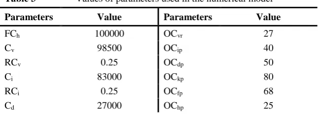
In this example, the parameter representing the cost of transportation between facilities is defined as the distance between facilities in the network. Moreover, the penalty costs of potential capacity and unsatisfied demand differ according to the relevant levels. The rest of the parameters used in this example are brought in Table (3).
Table 3 Values of parameters used in the numerical model
Value Parameters Value Parameters 27 OCvr 100000 FCh 40 OCip 98500 Cv 50 OCdp 0.25 RCv 80 OCkp 83000 Ci 68 OCfp 0.25 RCi 25 OChp 27000 Cd 3 2 1 2 3
max ( ( )
(
....
)
.
( )
( )
,
p pi i i
j j j
S
S
S
f x
r
r
r
s t
f
x
S
e
f
x
S
e
223
Table 3 Values of parameters used in the numerical model
27
RVv
12000
Ck
22
RPi
20000
Cf
uniform (800,1000)
PRcp
5000
Ch
3 NX
uniform (0.45,0.55)
TCcp
3 NY
0.05
TFf
3 NZ
3 Arp
2 NW
0.5 RT
2 NU
0.2 RF
0.1
RDVvr
0.45 RR
uniform (0.12,0.14)
RDIip
0.2 RV
650000
FCi
0.15 RH
125000
FCd
0.3 RIT
550000
FCk
143
CTdcpm
400000
FCf
uniform(4800,5200)
DCcp
In order to solve the proposed model using the augmented epsilon constraint method, the model must first be solved in single-objective mode. Therefore, three models with three discrete objectives of maximum profit, minimum time delays and minimum deterioration products and parts are solved. The maximum profit function is considered as the main objective function. Now the best and worst outputs values must be separately derived for each of the functions. To this end, the optimized outputs of each of these functions are used as inputs for other functions and thus the objective function is calculated. These values are presented in Table (4).
Table 4 Discrete values of objectives functions
deterioration products and parts
time delays profit
18742630 16727200
21518720 Profit
775 762
1049 time delays
15730 15785
16855 deterioration products and parts
224
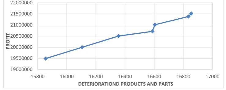
Fig 2 Value of maximum profit function against minimum deterioration products and parts
function
The profit in this figure is calculated against the amount of deterioration products and row materials. Profit would increase with the increase in the deterioration products. Indeed, with more raw materials being procured, more products would subsequently be manufactured and therefore more products would be sold to the customer which in turn increases the profit of network. However, since more raw materials are procured and more products have been manufactured, therefore the number of deterioration products would also increase.
Fig 3 Value of maximum profit function against minimum time delays function
Fig (3) represents the maximum profit function against the minimum time delays function. As the time delays increase, the profit also increases. In fact, the increase in the flow transmitted between the distributor and customer would lead to higher profit in the network. On occasions where more products are sold to the customers, the number of returned products would also increase. Therefore, more products would be dispatched to the repair centers and the transportation time from customer to collection, collection to repair, repair to distribution and distribution to customer centers would be increased and the time delays will also increase.
19000000 19500000 20000000 20500000 21000000 21500000 22000000
15800 16000 16200 16400 16600 16800 17000
PROF
IT
DETERIORATIOND PRODUCTS AND PARTS
19000000 19500000 20000000 20500000 21000000 21500000 22000000
900 920 940 960 980 1000 1020 1040 1060
PROF
IT
225
Fig 4 Minimum deterioration products and parts function against minimum time delays
Fig (4) depicts the minimum deterioration products function against the minimum time delays. With the increase in number of deterioration products, the time delays would also be increased. The increase in procurement of raw materials and manufactured products would subsequently lead to rise in number of deterioration d products and on the other hand, more products would be dispatched to repair center due to higher number of returned products and the time for repair of products and their transportation from customer to collection, collection to repair, repair to distribution and distribution to customer centers would be increased along with the overall time delay.
8.
Sensitivity Analysis
Diagrams (5) to (7) have been plotted to study the behavior of Pareto curve, amount of profit, time delays and number of deterioration products against the variations in deterioration rate percentage of raw materials. It should be noted that the variations in deterioration percentage of raw materials has been considered 0.1, 0.2 and 0.3.
Fig 5 Pareto curve of profit against the number of deterioration products and parts per
variations in percentage deterioration of raw materials.
As figure (5) suggests, the profit values of network would decrease due to increase in percentage of deterioration rate of raw materials and the number of deterioration products and parts would be increased. The rise in profit is due to the fact that the increase in deterioration rate of raw materials would lead to lesser number of parts dispatched from supply center to the manufacturing center resulting in less number of products and the subsequent less number of
15800 16000 16200 16400 16600 16800 17000
900 920 940 960 980 1000 1020 1040 1060
D
ETE
R
IO
R
A
TION
PRODUC
TS
A
N
D
PA
R
TS
TIME DELAYS
17000000 18000000 19000000 20000000 21000000 22000000
15000 16000 17000 18000 19000 20000
PROF
IT
DETERIORATION PRODUCTS AND PARTS
226
products sold to the customer the consequence of which is the decrease in overall profit of network.
Fig 6 Pareto curve depicting profit against time delays per percentage of deterioration rate
variations of raw materials.
Figure (6) suggests that the increase in percentage of deterioration rate of raw materials would result in decrease of profit and time delays. This decrease is due to the fact that deterioration he increase in deterioration rate of raw materials results in fewer parts is being dispatched to the manufacturing center and subsequently less number of products will be manufactured followed by less products sold to the customer and decrease in profit of the entire network. Moreover, as the sale of products to the customers decreases, the number of returned products is also decreased and thus fewer products are dispatched to the repair center. The repair time and transportation time from customer to collection, collection to repair, repair to distribution and distribution to customer centers would be decreased. Therefore, time delays would also be decreased.
Fig 7 Pareto curve depicting profit against time delays per percentage of deterioration rate
variations of raw materials
Considering Fig (7), the values of time delays and number of deterioration products and parts are respectively decreased and increased as a consequence of increase in percentage of deterioration rate of raw materials. The decrease in time delays is due to fewer numbers of parts dispatched to the factories because of increase in number of deterioration products and as a result fewer products are manufactured and subsequently less products are sold to the customer. Fewer sales would lead to decrease in returned products and less number of products dispatched to the repair center. The repair time and transportation time from customer to collection, collection to repair, repair to distribution and distribution to customer centers would be decreased. Therefore, time delays would also be decreased.
800 850 900 950 1000 1050 1100
17000000 18000000 19000000 20000000 21000000 22000000
TIM
E
D
EL
EYS
PROFIT
r=.1 r=.0.2 r=0.3
15000 16000 17000 18000 19000 20000 21000
800 850 900 950 1000 1050 1100
D
ETE
R
IO
R
A
TION
PRODUC
TS
A
N
D
PA
R
TS
TIME DELEYS
227
9.
Conclusions
A mixed integer nonlinear programming model is proposed in this article in both multi-product and multi-objective modes for the closed-loop logistics network. The entire potential centers in forward logistics include supply, manufacturing, distribution and customer center while collection, recycling, reproduction, repair and disposal centers are considered in the reverse logistics so that the developed model may be closer to the real world since there are only a few models that have incorporated all these centers. The objectives of proposed model are to maximize profit, minimize time delays and minimize deterioration rate of products and parts. The costs considered in this model include those of establishment and construction of facilities, procurement of raw materials, transportation and flow between facilities, penalties of unsatisfied demands and unfulfilled potential capacities. The outputs of model consist of location of facilities, optimized flow between facilities, unsatisfied demand, the minimum number of vehicles used between distribution and customer facilities, procurement of raw materials and number of manufactured products. Augmented epsilon constraint method was used to solve the multi-objective model and a numerical example was provided and analyzed to determine the accreditation and applicability of this proposed model. Furthermore, the results derived from solution of multi-objective model verify the results from single-objective models and approves the efficiency of the applied technique.
For future research in this area, we suggest the development of some heuristic and meta-heuristic methods for large-sized problems as well as exact decomposition techniques. Furthermore, the model can be improved with several extensions, such as addressing risk, budget constraints and considering uncertainty mode or various time periods as well as other objectives such as level of response, quality level of products and others may be recommended for future studies.
Acknowledgements
The authors would like to thank to anonymous referees and their valuable comments, which helped to improve the quality of this paper.
10.
Reference
Amin, S.H. and Zhang, G., (2012). “An integrated model for closed-loop supply chain
configuration and supplier selection: Multi-objective approach”, Expert Systems with
Applications, Vol. 39, No. 8, pp. 6782-6791.
Amin, S.H. and Zhang, G., (2013). “A multi-objective facility location model for closed-loop
supply network under uncertain demand and return”, Applied Mathematical Modelling,
Vol.37, No. 6, pp. 4165-4176.
Amiri, A. (2006), “Designing a distribution network in a supply chain system: formulation and
efficient solution procedure”, European Journal of Operational Research, Vol.171, No.
2, pp. 567–576.
228
Bernon, M. and Cullen, J. (2007). “An integrated approach to managing reverse logistics.”
International Journal of Logistics: Research and Applications, Vol. 10, No. 1, pp. 41-56.
Demirel, N., Ozceylan, E., Paksoy, T. and Gokcen, H., (2014). “A genetic algorithm approach for optimizing a closed-loop supply chain network with crisp and fuzzy objectives”,
International Journal of Production Research, Vol.52, No. 12, pp. 3637-3664.
Eskandarpour M, Zegordi S.H. and Nikbakhsh E. (2012), “A parallel variable neighbourhood search for the multi-objective sustainable post-sales network design problem”,
International Journal of Production Economics, Vol. 145, No. 1, pp. 117–131.
Fallah-Tafti, A., Sahraeian, R., Tavakkoli-Moghaddam, R. and Moeinipour, M., (2014). “An interactive possibility programming approach for a multi-objective closed-loop supply
chain network under uncertainty”, International Journal of Systems Science, Vol.45, No.
3, pp. 283-299.
Fleischmann, M., Beullens, P., Bloemhof-Ruwaard, JM., and Wassenhove, L. (2001). “The impact of product recovery on logistics network design.” Production and Operations Management, Vol. 10, No. 2, pp. 156-173.
Ghorbani, M., Arabzad, S.M. and Tavakkoli-Moghaddam, R. (2014). “A Multi-objective
Fuzzy Goal Programming Model for Reverse Supply Chain Design”, International
Journal of Operational Research, Vol. 19, No.2, pp. 141-153.
Hatefi, S.M., F. Jolai, (2013). “Robust and reliable forward–reverse logistics network design under demand uncertainty and facility disruptions,” Applied Mathematical Modelling, Vol. 38, No. 9–10, PP. 2630-2647.
Hatefi, S.M. and Jolai, F. (2014). “Robust and reliable forward–reverse logistics network
design under demand uncertainty and facility disruptions”, Applied Mathematical
Modelling, Vol. 38, No. 9, pp. 9-10.
Keyvanshokooh, E., Fattahi, M., Seyed-Hosseini, S.M., and Tavakkoli-Moghaddam, R., (2013).“A dynamic pricing approach for returned products in integrated forward/reverse
logistics network design”, Applied Mathematical Modelling, Vol. 37, No. 24, pp.
10182-10202.
Lee, D.H. and Dong, M. (2008). “A heuristic approach to logistics network design for
end-of-lease computer products recovery”, Transportation Research E, Vol. 44, No. 3, pp.
455-474.
Mavrotas, G. and Florios, K., (2013), “An improved version of the augmented ε-constraint method (AUGMECON2) for finding the exact pare to set in multi-objective integer
programming problems”, Applied Mathematics and Computation, Vol. 219, No.18, pp.
9652-9669.
Özceylan, E., Paksoy, T. and Bektaş, T. (2014). “Modelling and optimizing the integrated problem of closed-loop supply chain network design and disassembly line balancing”,
Transportation Research Part E: Logistics and Transportation Review, Vol. 61, No. 1,
pp.142-164.
Pishvaee, M. S., Rabbani, M., and Torabi, S. A. (2011). “A robust optimization approach to
closed-loop supply chain network design under uncertainty”, Applied Mathematical
Modelling, Vol. 35, No. 4, pp. 637–649.
229
Pishvaee, M.S., Razmi, J. and Torabi, S.A., (2014). “An accelerated Benders decomposition algorithm for sustainable supply chain network design under uncertainty: A case study of medical needle and syringe supply chain”, Transportation Research Part E: Logistics and Transportation Review, Vol. 67, No. 1, pp. 14-38.
Ramezani, M., Bashiri, M. and Tavakkoli-Moghaddam, R., (2013). “A new multi-objective stochastic model for a forward/reverse logistic network design with responsiveness and
quality level”, Applied MathematicalModel, Vol. 37, No. 1-2, pp. 328-344.
Ramezani, M., Kimiagari, A.M., Karimi, B. and Hejazi, T.H., (2014). “Closed-loop supply
chain network design under a fuzzy environment”, Knowledge-Based Systems, Vol. 59,
No. 1, pp. 108-120.
Santoso T, Ahmed S, Goetschalckx M. and Shapiro A. (2005). “A stochastic programming
approach for supply chain network design under uncertainty”, European Journal of
Operational Research, Vol. 167, No. 1, pp. 96-115.
Tabrizi, B.H. and Razmi, J., (2013). “Introducing a mixed-integer non-linear fuzzy model for
risk management in designing supply chain networks”, Journal of Manufacturing
Systems, Vol. 32, No. 2, pp. 295-307.
Vahdani, B., Razmi, J. and Tavakkoli-Moghaddam, R. (2012), “Fuzzy possibility modelling
for closed-loop recycling collection networks”, Environmental Modelling and
Assessment, Vol. 17, No. 6, pp. 623–637.
Vahdani, B., Tavakkoli-Moghaddam, R., Jolai, F. and Baboli, A., (2014). “Reliable design of
a closed loop supply chain network under uncertainty”, an interval fuzzy possibility