Estimation of LLE Data for Binary Systems of N-Formylmorpholine with Alkanes Using Artificial Neural Network–Genetic Algorithm (ANN–GA) Model

*Corresponding author: E-mail: [email protected]

Department of Chemical Engineering, Faculty of Engineering, University of Kurdistan, Sanandaj, Iran

Chemical Methodologies 3(2019) 67-82

Chemical Methodologies

Journalhomepage: http://chemmethod.com

Original Research article

Estimation of LLE Data for Binary Systems of

N-Formylmorpholine with Alkanes Using Artificial Neural

Network–Genetic Algorithm (ANN–GA) Model

Reza Beigzadeh

Department of Chemical Engineering, Faculty of Engineering, University of Kurdistan, Sanandaj, Iran

A R T I C L E I NF O R MA T I O N A B S T R A C T Received: 24 May 2018

Received in revised: 22 August 2018

Accepted: 10 September 2018 Available online: 10 September 2018

DOI:

10.22034/CHEMM.2018.133293.1059

The purpose of this work was to predict liquid-liquid equilibrium of binary systems including N-formylmorpholine (NFM) with alkanes (heptane, nonane, and 2,2,4-trimethylpentane) over the temperature range from around 300 K to 420 K. Therefore, three feed-forward artificial neural network (ANN) models were developed for the three systems. Compositions of alkanesin light phase and heavy phase were considered as network inputs, and the temperature was the output variable. Genetic algorithm (GA) method was used to design the neural network. It minimized the total mean squared error (MSE) between net output and desired output with optimizing weights and biases of the ANN. The validity of the models was evaluated through a test data set, which was not used in the training data set. The results of this work show that the hybrid of artificial neural network and genetic algorithm (ANN–GA) can estimate the LLE of the binary systems with high precision. KEYWORDS

Artificial neural network (ANN) Binary system

Genetic algorithm (GA) Liquid-liquid Equilibrium (LLE)

Graphical Abstract

Introduction

gasoline and refines the extracted aromatics. Thus, NFM plays an important role in liquid extraction and has a model for predicting phase equilibrium and thermodynamic properties of systems containing morpholine whose derivatives are essential.

For a better understanding of their thermodynamic behavior and for the development of the model, trustworthy experimental phase equilibrium data are needed. Therefore, several researchers started with measurements of the required properties of the liquid-liquid equilibrium. Some LLE data of binary systems including NFM with n-alkanes [8-13] and cycloalkanes [10] and some of the ternary systems including NFM, aromatics, and alkanes [14-17] have been investigated. Some experimental LLE data for a mixed solvent system (N-formylmorpholine + sulfolane, n-hexane and benzene) over the temperature range of 298.15 to 318.15 K were determined by J. Mahmoudi and M.N. Lotfollahi [18]. The LLE data of NFM with aromatics, n-hexane, n-heptaneand water at different temperatures from 293 to 333 K were obtained by Cincotti et al. [8]. The LLE results for the ternary mixture of (NFM + 2,2,4-trimethylpentane + ethylbenzene) at temperatures 303.15, 313.15, and 323.15 K were investigated by Z. Wang et al. [1]. However, according to the importance of NFM, the liquid-liquid equilibrium data are still comparatively scarce for the binary systems containing NFM in the studies; and a mathematical model with the aim of contributing to the knowledge of liquid-liquid equilibrium with NFM can be so useful. There are limited empirical correlations for predicting LLE characterization. On the other hand, the artificial neural network (ANN) models on VLE data in several subjects have been carried out [19-21] but there are limited studies on LLE data using ANN models.

Experimental

Hybrid neural networks and genetic algorithm

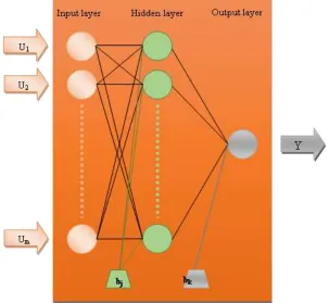
Artificial neural networks (ANNs) which are collections of flexible mathematical functions imitate biological systems using a number of interconnected artificial neurons to recognize complex and nonlinear relationships [24]. Because of this ability of the ANNs, they can be used in various fields of chemical engineering [25]. The ANN learns the data pattern using the “training” algorithms. These methods are extremely useful in recognizing templates in complex data by providing non-linear equations between inputs and outputs of the network. Each neuron of the network is connected with a weight to the other neurons via direct communication bonds, which finally provides a reasonable relationship between input and output values. The output of each neuron generated by summation of weighed inputs plus bias under a transfer function. In common, ANNs are parallel organized structures that comprised of interconnected neurons as input layer (independent variables), one or more hidden layers, be located between them, and an output layer (dependent variables) [26] as shown in Figure 1. The number of neurons of the input and output layers is usually determined by the number of input and output variables (U and Y), respectively. However, the number of neurons in the hidden layers is changeable and it is important for optimization of the network, which will be studied in the following sections.

biases of the BP network is the genetic algorithm (GA) [28]. In this work, the initial weights and biases of the artificial neural network were optimized using this method.

Figure 1. Topology of three-layer back propagation artificial neural network used in this study

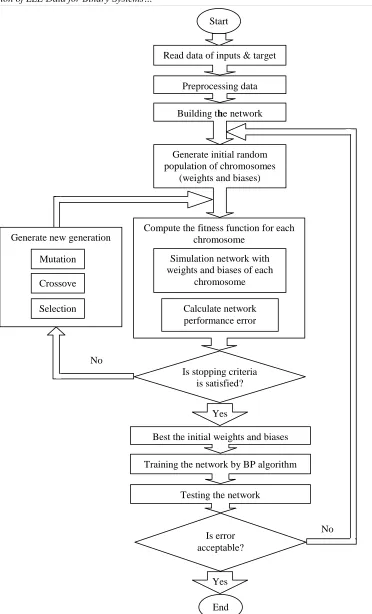
GA is an extremely important method in optimization inspired by Darwinian biological evolution principle, which is quite popular in engineering optimization. The optimization procedure involves selection, elitism, crossover, and mutation operations and starts with a set of random solution (population) and develops through continuous iterations (generations) for getting better solutions [27-29]. In brief, GA uses four steps to obtain the optimum weights of ANN as follows [22-30]: Generate random initial population of chromosomes (weights and biases).

Evaluate the fitness values (objective function value) of solutions (computing their performance error).

Represent new generation by selection, elitism, crossover, and mutation.

Figure 2. Flowchart of the artificial neural network–genetic algorithm (ANN–GA) model

No

No Is stopping criteria

is satisfied?

Yes

Best the initial weights and biases

Training the network by BP algorithm

Testing the network Start

Generate initial random population of chromosomes

(weights and biases) Read data of inputs & target

Preprocessing data

Building the network

Compute the fitness function for each chromosome

Simulation network with weights and biases of each

chromosome

Calculate network performance error

End Is error acceptable?

Yes Generate new generation

Selection Crossove

The final step in designing ANN is to test the performance of the model. At this step, test data are used in the ANN model and in order to evaluate the performance of the model, the mean relative error (MRE) and the mean square error (MSE) between the experimental and estimated values were measured. Figure 2. shows the flow chart of the artificial neural network–genetic algorithm (ANN–GA) model which has been used in this work.

Developing correlations using ANN-GA modeling and training

The ANN that is used in this study is a multilayer feed-forward neural network with the Levenberg-Marquardt algorithm [31-33] for the correction of the weights and a learning order of the back propagation (BP) of errors.

The experimental LLE data for three mixtures composed of N-formylmorpholine (NFM) with alkanes (heptane, nonane, and 2,2,4-trimethylpentane) over the temperature range from around 300 K to 420 K, were measured by Wang et al. [23] and were used for training and testing the ANN-GA model. The investigated systems were at the equilibrium condition. There were two components in each of the systems, N-formylmorpholine (NFM) with an alkane. In this study, the ANN was developed for predicting temperature (output data) as a function of mole fraction of alkane in light phase (X11) and mole fraction of alkane in heavy phase (X12) (input data). Before the

training of the ANNs, because of the different range sizes between input and output data, it is usually common to normalize input and output data. So, all data were normalized in the range of 0-1 in order to avoid any computational difficulty, using the following relation:

value minimum value

maximum

value minimum value

data data

Normalized

  

(1)

In the neural network model, the final output of the ANN is obtained from the following relationship [35]:                       







 i j k

m 1 i i j t n 1 j j k

l W F W U b b

F Y

(2)

here Y, U, m, n are the final answer of the network, the input value of the network, the number of input variables and the number of neurons; ‘i’, ‘j’ and ‘k’ refer to the input, hidden, and output layer, respectively. In this study, the “hyperbolic tangent sigmoid” transfer function was chosen for the hidden layer and “linear” function was considered for the output layer. These functions are defined as follows:

1

e

1

2

(x)

F

_{t 2x}







_

(3)

x

(x)

F

_l



₍₄₎

As mentioned for training networks, random initial weights and biases may cause trapping into local minima and converge slowly. So in this study, GA searching approach was used for solving problems on which traditional methods do not succeed to achieve the global optimum result (minimum or maximum). Based on results, the best population size in the case studied here was found to be 100. The crossover probability and mutation probability are determined and their values were found to be 0.8 and 0.01, respectively. The GA would stop after the end of 300 generations because it had almost reached optimal values.

For evaluating the validity of the model, the data points were divided randomly into two parts, the first data set (around 70% of input data) was selected for training the network and the second data set (remaining data) was employed for testing the model.

Results and discussion

Table 1. Experimental LLE data of temperature at the mole fraction of light phase x11 and heavy phase x12 for

the system {Nonane (1) + NFM (2)} [11]

T/K Light phase x11 Heavy phase x12 T/K Light phase x11 Heavy phase x12

303.15 0.9801 0.0118 365.85 0.8952 0.0226

312.95 0.9661 0.0148 370.95 0.8841 0.0289

320.65 0.9572 0.0176 392.45 0.8344 0.0346

327.97 0.9484 0.0192 402.15 0.8107 0.0347

334.95 0.942 0.0212 409.65 0.7979 0.0373

343.04 0.9322 0.0219 415.25 0.7886 0.0386

350.65 0.9236 0.0202 427.85 0.7621 0.0433

356.95 0.9098 0.0213

Table 2. Experimental LLE data of temperature at the mole fraction of light phase x11 and heavy phase x12 for

the system {2,2,4-trimethylpentane (1) + NFM (2)} [11]

T/K Light phase x11 Heavy phase x12 T/K Light phase x11 Heavy phase x12

307.85 0.9705 0.0193 355.55 0.8838 0.0316

312.55 0.9673 0.022 365.25 0.8677 0.0382

318.85 0.964 0.0248 374.55 0.8426 0.0417

323.64 0.9577 0.0263 383.75 0.804 0.0413

329.33 0.9542 0.0273 391.65 0.7784 0.0428

334.85 0.9447 0.0289 399.65 0.7595 0.047

342.5 0.9313 0.0298 408.45 0.7401 0.0504

349.4 0.9134 0.0311

Table 3. Experimental LLE data of temperature at the mole fraction of light phase x11 and heavy phase x12 for

the system {heptane (1) + NFM (2)} [11]

T/K Light phase x11 Heavy phase x12 T/K Light phase x11 Heavy phase x12

298.75 0.9794 0.0183 348.35 0.9527 0.0399

302.85 0.9688 0.0216 357.75 0.9467 0.0446

312.05 0.9645 0.0243 369.35 0.9279 0.0536

320.05 0.9624 0.0277 378.3 0.9087 0.0667

329.35 0.9605 0.0323 389.35 0.8819 0.0804

337.65 0.9575 0.038

neurons was evaluated. The deviation, which was used for choosing the best ANN architecture, is the mean square error (MSE) defined as follow:









N

i

i

i

y

)

t

(

N

MSE

1

2

1

(5) Where N is the number of data points, t is the target (experimental) data, and y is the estimated value.

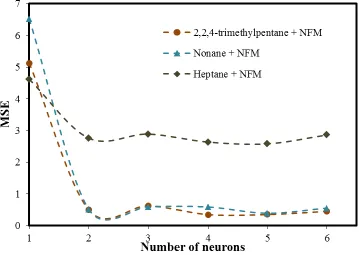
The results of the method for achieving the optimum number of neurons in the hidden layer have been presented in Figure 3. In the Figure, MSE values of different ANN configurations, of each the three networks, for estimation of T are presented. The configuration with minimum error (MSE) is determined as the best network architecture. According to Figure 3, the best network configuration has one hidden layer with two neurons. The minimum MSE values of the ANN for the prediction of system temperature were 0.5168, 2.7606 and 0.5034, for (nonane + NFM), (heptane + NFM) and (2,2,4-trimethylpentane + NFM) systems, respectively.

Figure 3. MSE values for different number of hidden neurons in the developed ANNs

Hence, for the three LLE systems, the final output of the ANN-GA via input compositions can be obtained using the parameters (weights and biases) of the selected ANN architecture in Eq. (2), as follows:

nonane (1) + NFM (2) {:









5669 . 0 7356 . 3 2642 . 0 x 4.4314 -F 3029 . 0 0777 . 0 x 2597 . 0 x 9987 . 1 F 4015 . 0 T 12 11 t 12 11 t         x (6) 2,2,4

-} trimethylpentane (1) + NFM (2) {:









5234

.

0

3842

.

0

0019

.

1

x

5114

.

1

F

3842

.

0

1788

.

3

x

8823

.

1

x

8521

.

3

F

2648

.

0

T

12 11 t 12 11 t

















x

(7)

} heptane (1) + NFM (2) {:









7121 . 0 6428 . 0 2434 . 0 x 7517 . 1 F 3662 . 0 0153 . 2 x 0468 . 2 x 1796 . 3 F 4280 . 0 T 12 11 t 12 11 t         x (8) It should be noted that input and output data are in normalized range (Eq. 1). Table 4. reports the MSE and MRE values of the systems with optimum hidden neurons and same iterations. The MSE equation mentioned as Eq. (5) and mean relative errors (MRE) calculated as follows:



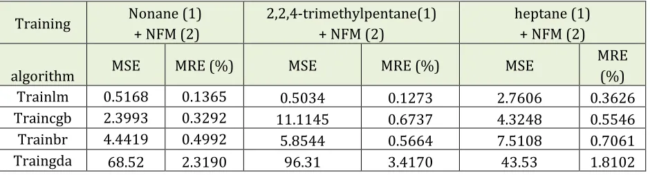
        N i i i i t y t N MRE 1 100 (%) (9) Where N, t and y parameters are the number of data points, the target (experimental) data, and the estimated value, respectively, alike in MSE equation.

Table 4. Best MSE and MRE values of different training algorithm for ANNs with 2-2-1 configuration

Training Nonane (1) + NFM (2)

2,2,4-trimethylpentane(1) + NFM (2)

heptane (1) + NFM (2)

algorithm MSE MRE (%) MSE MRE (%) MSE

MRE (%)

Trainlm 0.5168 0.1365 0.5034 0.1273 2.7606 0.3626

Traincgb 2.3993 0.3292 11.1145 0.6737 4.3248 0.5546

Trainbr 4.4419 0.4992 5.8544 0.5664 7.5108 0.7061

Traingda 68.52 2.3190 96.31 3.4170 43.53 1.8102

bayesian regularization back–propagation (trainbr), and gradient descent with adaptive learning rate back-propagation (traingda). The obtained errors in this table revealed that using the Levenberg-Marquardt algorithm (trainlm) leads to the best answer.

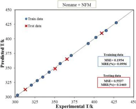
The comparison between the simulation results for prediction of temperature for the developed ANN-GA and the experimental training data points is illustrated in Figure 4. It is tried to illustrate the validity of the model in the prediction of the temperature for {nonane (1) + NFM (2)} mixture. The best fit, that output is equal to targets, is appeared by the solid line. Figure 4. shows a good correlation between the ANN predictions and the experimental data and it indicates that the neural network estimated values are close to the experimental data for all data points. Also, the accuracy of the developed network has been tested by using the test data set, which was not used for the training step. In addition, the evaluations indicate that the MSE and MRE for the training data are 0.1954 and 0.0996, respectively, and for the test data are 0.5537 and 0.1460, respectively.

Figure 4. Scatter diagram showing the performance of Eq. (1) for predicting the (liquid-liquid) equilibrium data of the {nonane (1) + NFM (2)} mixture

respectively, for the {heptane (1) + NFM (2)} mixtures. This means that the hybrid neural network and the genetic algorithm was also suitable for predicting the data points which are not used in the training data set.

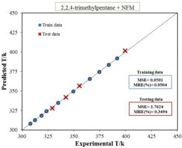
Figure 5. Scatter diagram showing the performance of Eq. (2) for predicting (liquid-liquid) equilibrium data of the {2,2,4-trimethylpentane (1) + NFM (2)} mixture

Conclusion

In the present study, three ANN–GA models were developed for three systems including N -formylmorpholine (NFM) with alkanes (heptane, nonane, and 2,2,4-trimethylpentane) in order to predict the temperature (T) in liquid-liquid equilibrium conditions. The value of T was used as a function of the primarily influencing parameter, mole fraction of the alkane in light phase (X11) and

mole fraction of alkane in heavy phase (X12) which were considered in the inputs of the networks.

In this work, the hybrid neural network and genetic algorithm were successfully applied to estimate the LLE characteristics. Three sets of experimental data points were used for training the feed-forward neural network. The best architecture for the network has one hidden layer with two neurons which is obtained by trial and error. GA which can be regarded as one of the most effective techniques is used for optimizing the initial weights and biases of the ANN network. This method was applied as a very useful technique in the design of the network. The performance of the proposed ANN-GA model was also examined through is application in a test data set consisting of about one-third of the experimental data not used for training. The results of applying the hybrid of artificial neural network and genetic algorithm (ANN-GA) model show that the method has a very good performance in estimating the LLE data of the binary systems containing N -formylmorpholine.

List of symbols

b :bias w : weight

F : transfer function

m : number of input variables n : number of neurons

N : number of data points t : target

T : temperature [K]

U : input value of the network Y : final answer of the network

Subscripts

References

[1] Houshyar S., Torab-Mostaedi M., Moosavian S.M.A., Mousavi S.H., Asadollahzadeh M. Iran. J. Chem. Eng., 2017, 14:82

[2] Hassan M.S., Fahim M.A., Mumford C.J. J. Chem. Eng. Data, 1988, 33:162 [3] Cele N.P., Bahadur I., Redhi G.G., Ebenso E.E. J. Chem. Thermody., 2016, 96:169 [4] Ko M., Im J., Sung J.Y., Kim H. J. Chem. Eng. Data, 2006, 51:636

[5] Im J., Lee H., Lee S., Kim H. Fluid Phase Equilib., 2006, 246:34

[6] Symoniak M.F., Ganju Y.N., Vidueira J.A. Hydrocarbon Process., 1981, 60:139 [7] Nicolae M., Oprea F., Fendu E.M. Chem. Eng. Res. Des., 2015, 104:287

[8] Cincotti A., Murru M., Cao G., Marongiu B., Masia F., Sannia M. J. Chem. Eng. Data, 1999, 44:480 [9] Chen D., Ye H., Hao W. J. Chem. Thermodyn., 2007, 39:1571

[10] Ko M., Na S., Lee S., Kim H. J. Chem. Eng. Data, 2003, 48:249 [11] Mahmoudi J., Lotfollahi M.N. Korean J. Chem. Eng., 2010, 27:214

[12] Mahmoudjanloo H., Izadpanah A.A., Osfouri S., Mohammadi A.H. Chem. Eng. Sci., 2013, 98:152 [13] Mahmoudjanloo H., Izadpanah A.A., Rajaei H., karamian S., Esmaeilzadeh F. Fluid Phase Equilib., 2016, 408:38

[14] Abrams D.S., Prausnitz J.M. AIChE J., 1975, 21:116

[15] Domínguez I., González E.J., Palomar J., Domínguez Á. J. Chem. Thermody., 2014, 77:222 [16] HorstmannS., Fischer K., Gmehling J., Kolář P. J. Chem. Thermody., 2000, 32:451

[17] De Los Ríos A.P., Hernández Fernández F.J., Gómez D., Rubio M., Víllora G. Sep. Sci. Technol.,

2012, 47:300

[18] Behrooz H.A., Boozarjomehry R.B. Fluid Phase Equilib., 2017, 433:174 [19] Fernández L., Ortega J., Wisniak J. Comput. Chem. Eng., 2017, 106:437 [20] Roosta A., Hekayati J., Javanmardi J. Neural Comput. Appl., 2017, p 1

[21] Fazlali A., Koranian P., Beigzadeh R., Rahimi M. Korean J. Chem. Eng., 2013, 30:1681 [22] Karimi H., Yousefi F. Fluid Phase Equilib., 2012, 336:79

[23] Wang Z., Xia S., Ma P., Liu T., Han K. J. Chem. Thermody., 2012, 47:228

[24] Hagan M.T., Demuth H.B., Beale, M.H. Neural network design; PWS Pub. Co.: Boston, 1996 [25] Hussain M.A. Artif. Intell. Eng., 1999, 13:55

[26] Basheer I.A., Hajmeer M. J. Microbiol. Method., 2000, 43:3

[27] Beigzadeh R., Rahimi M., Parvizi M., Eiamsa-ard S. Numer. Heat. Trans. A- Appl., 2014, 65:186 [28] Chang Y.T., Lin J., Shieh J.S., Abbod, M.F. Adv. Fuzzy System., 2012, 2012: 1-9

[30] Yazdanmehr M., Mousavi Anijdan S.M., Bahrami A. Comput. Mater. Sci., 2009, 44:1218 [31] Levenberg K. SIAM J. Numer. Anal., 1944, 16:588

[32] Marquardt D.W. J. Soc. Indust. Appl. Math., 1963, 11:431 [33] Hagan M.T., Menhaj M.B. IEEE Trans. Neural Net., 1994, 5:989 [34] Haykin S. Neural Networks; M. Horton ed., 1999

[35] Renon H., Prausnitz J.M. AIChE J., 1968, 14:135