A simple 2-D interpolation model for analysis of
nonlinear data
Mehdi Zamani
Department of Civil Engineering, Faculty of Technology and Engineering, Yasouj University, Yasouj, Iran; [email protected]
Received 1 March 2010; revised 24 April 2010; accepted 13 May 2010.
ABSTRACT
To determination the volume and weight of non- uniform bodies, such as in ore deposits evalua-tion for mining and rock cutting for construcevalua-tion, the methods of interpolation are usually used. The classic curves, which are frequently used to interpolate one-dimensional data are cubic spl- ine, Bspline and Bezier curves. These methods have good efficiency for determination of geom- etric characteristics of nonregular masses. They have some limitations and problems with two- dimensional interpolation analysis such as for- ming large linear systems of equations with a lot of entries and difficulty encounter with their solutions. In this research the two-dimensional splines are used, which have the advantages of simplicity and less computational operations ef- fort. The spline functions that are applied have the continuity of C1 at elements boundaries. The presented model has suitable efficiency for vo- lumes of large extents governing to lots of data. Keywords:Simulation; Approximation; Least square; Cubic Spline; Optimization; Curve Fitting; Prediction
1. INTRODUCTION
The most popular methods for interpolation of data are Lagrange method, Neville iteration approach, Newton divided difference methods, Cubic spline, Hermit spline, Bspline and Bezier methods. For the Neville and New-ton divided difference method, the higher degree of pol- ynomial generation is straightforward. In conic spline approach each curve consists of a number of about n segment curves. The general way is to divide the interval to collect subintervals or segments and construct differ-ent approximating polynomial on each interval. Appr- oximation by functions of this type is called piecewise
polynomial approximation. This method has the advan-tage of removing the oscillatory nature of high degree polynomials. In this approach there exists the continuity of C2 on the segments boundaries. However; the conti-nuity order is optional to users willing. The formulation for creating cubic spline curve results in the solution of a three-diagonal system of equations. Hermit interpolation are based on two points p1 and p2 and two tangent values
' 1
p and ' 2
p at those points. It computes a curve seg-ment that starts at p1, going in direction to p1' and ends at p2 moving toward p2'. Hermit interpolation has an important advantage. The Hermit curve can be modified by changing the tangent values.
The Bezier curve is a parametric curve p(t) that is a polynomial function of the parameter t. The degree of the polynomial depends on the number of points used to define the curve. The method applies control points and presents an approximating curve. The Bezier curve does not pass through internal points but the first and last points. Internal points influence the direction and posi-tion of the curve by pulling it toward themselves [1-3]. B-spline methods were first proposed in the 1940 for curves and surfaces. The B-spline curves can be ap-proximating or interpolating curves. The advantage of B-spline curves to Bezier curve is the obtaining the higher continuity for the individual spline segments [2-5]. If there are a set of triple data {( , , '),
i i i y y
x c
} , , 2 , 1 ,
0 n
i The cubic spline functions Si(x) can be obtained on each interval [xi, xi+1]. With this model the continuity of C1 exists on the boundary of each segment. The spline function of degree 3 for each interval is:
i i i i
i i i i i
d c b a
x x x x
d x c x b a x
g ( ) 2 3 1 2 3 (1)
i i i i
i i i
i i i
i i i i i i i i
d c b a
x x x
x x x
x x x
x x d x x c x x b a x s
1 0 0 0
3 1 0 0
3 2 1 0 1 1
) ( ) ( ) ( )
(
2 2 3 2
3 2
3 2
(2)
The first derivatives of the spline function (2) is as follows,
i i i
i i i
i i i i i i
d c b x x x x
x
x x d x x c b x s
3 0 0
6 2 0
3 2 1 1
) ( 3 ) ( 2 )
(
2
2
2 '
(3)
The coefficients ai,bi,ci and difor each interval can be obtained explicitly from the Eq.5.
) (
1 ) (
2
) 2 ( 1 ) (
3
) (
) (
' '
1 2 1
3
' '
1 1
2
' '
i i i i i i i
i i i i i i i
i i i
i i i
f f h f f h d
f f h f f h c
f x s b
f x s a
, (4)
where hi is the element size or the element interval (hi =
xi+1 – xi). The problem with this approach is that we generally don’t have the tangent values at n + 1 point. This can be provided by applying the following ap-proximation equations (forward difference, central dif-ference and backward difdif-ference approximation, respec-tively) for the first derivatives at the points and for uni-form intervals hi.
] 3 , 4 , 1 [ 2
1
] 1 , 0 , 1 [ 2
1
] 1 , 4 , 3 [ 2
1
' ' '
i i
i i
i i
h f
h f
h f
, (5)
The following two examples show the interpolation of two sets of data by the above approach.
2. EXAMPLES
2.1. Example 1
This example is in the field of groundwater engineering. When a production well in unconfined aquifer is pumped, water is continuously withdrawn from storage within the aquifer as the cone of depression progresses radially outward from the well. Because of the absence of a
re-charge source in the form of vertical leakage, there can be no stabilization of water levels and the head (h) in the aquifer will continue to decline supposing the aquifer is infinite in areal extent. However, the rate of decline of head (h) continuously decreases as the cone of depres-sion spreads. The partial differential equation governing the unsteady-state radial flow in the nonleaky confined aquifer in polar coordinate system is,
t h T S r h r r
h
1
2 2
. (6) The Theis solution for the above partial differential equation is,
du u e T Q h h s
u u
4
0 . (7) Theis approximated the above equation by the fol-lowing series,
! 3 3 ! 2 2 log
5772 . 0 4
3 2
0
u u u u T
Q h
h e
(8) where,
Tt S r u
2 87 . 1
s = drawdown, in feet, Q = discharge, in gpm,
t = time after pumping started, in days,
T = coefficient of transmisivity, in gallons per day per foot (gpd/ft) and
S = coefficient of storage, dimensionless.
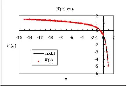
The value of brackets equals W(u). The data for in-terpolation have logarithm values of W(u) respect to u [6]. For the interpolation of data about ten points are considered. Figure 1 shows the comparison between the
W(u) vs u
W(u)
u
[image:2.595.315.534.547.695.2]model W(u)
data and the model for the nine spline curves. Based on the figure there is a suitable and good relationship be-tween those.
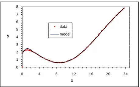
2.2. Example 2
In this problem about five pairs of data are obtained from the parametric Eq.9 with non-uniform segments.
] 24 , 0 [ , 12 cos 2 sin 2 12 sin
12 sin 2 sin 2 12 cos
t t
t y
t t
x
. (9)
About four cubic spline curves are generated accord-ing to the formulations of Eqs.3, 4 and 5. Figure 2 shows the relationship between the real values and in-terpolated ones. As it can be seen, there is a relative ex-pectable fitness between them.
3. FORMULATION FOR 2-D
INTERPOLATION
The bicubic spline formation that applies hear for two dimensional interpolation and four nodes patch is,
2 2 3
0 1 2 3 4 5 6
2 2 3
7 8 9
( , ) ij
g x y a a x a y a x a xy a y a x a x y a xy a y
(10) or in matrix notation,
3 2
6 7 3
8 4 1
9 5 2 0
3 2
1
0 0 0
0 0
0 1 )
, (
y y y
a a a
a a a
a a a a
x x x y A x y x gij
.
(11)If the above equation is written based on (xi,yi) or the coordinates of the lower left point on each segment, Eq.12
y
[image:3.595.57.287.558.702.2]x
Figure 2. The comparison between the data and the model.
obtains. Then, the formulation for determination of the coefficient will be simpler.
2
0 1 2 3
2
4 5
3 2
6 7
2 3
8 9
( , ) ( ) ( ) ( )
( )( ) ( )
( ) ( ) ( )
( )( ) ( )
ij i j i
i j j
i i j
j j j
s x y a a x x a y y a x x a x x y y a y y a x x a x x y y a x x y y a y y
(12)
or in matrix notation it is,
3 2 2
3 2
2 3 2
3 2
1
1 3 3
0 1 2
0 0 1
0 0 0 1
1 0 0 0
3 1 0 0
3 2 1 0 1
1 ) , (
y y y
y y
y y y
y A
x x x
x x
x
x x x y
x s
i i
i i i
i
i i i
i i i
ij
.
(13) The above bispline function has ten parameters (un-knowns) for each segment or patch. Therefore; ten equa-tions are required for defining them. Four equaequa-tions sat-isfy the function values at each corner and six equations satisfying partial derivative in x and y directions for three nodes. Thus there exists the continuity of C1 on each of four sides or boundaries of every element. The first derivatives in x and y direction for the Eq.12 are:
2 2
6 7 3
8 4 1
2 2
1
1 2
0 1
0 0 1
0 0
0
1 0 0
3 1 0
3 2 1 3 2 1 ) , (
y y y
y y a
a a
a a a
x x x x
x x
y x s
j j
j
i i i ij
.
(14)
2 2
7 8 4
9 5 2
2 2
3 2
1
1 3 3
0 1 2
0 0 1
0 0
0
1 0 0
2 1 0 1 1
) , (
y y y
y y a
a a
a a a
x x x x
x y
y x s
j j
j i i i ij
.
' , 2 ' , 1 0 ) , ( , ) , ( , ) , ( ij y ij ij x ij ij ij f a y j i s f a x j i s f a j i s (16) ' , 1 , 6 2 3
1 2 3
) , 1
( i i xi j
ij f a h a h a j i x s
, (17) ' 1 , , 9 2 5
2 2 3
) 1 , ( j i y j j ij f a k a k a j i y s
, (18) ' , 1 , 7 2 4 2 ) , 1
( i i yi j
ij i j a h a h a f
y s
, (19) ' 1 , , 8 2 4 1 ) 1 , ( j i x j j
ij i j a k a k a f
x s
, (20)
j i i i i j i ij f a h a h a h a j i s j i s , 1 6 3 3 2 1 0 ,
1 ( 1, )
) , 1 (
, (21)
1 , 9 3 5 2 2 0 1 , (, 1) ) 1 , ( j i j j j j i ij f a k a k a k a j i s j i s
, (22)
1 , 1 9 3 8 2 7 2 6 3 5 2 4 3 3 2 1 0 1 ,
1 ( 1, 1) ) 1 , 1 ( j i j j i j i i j j i i j i j i ij f a k a k h a k h a h a k a k h a h a k a h a j i s j i s (23)
The above ten equations give a linear system of equa-tions. If it is solved analytically the governing parame-ters are obtained as follows,
, 1 3 2 3 ' 1 , , 1 2 1 0 2
3 xi j
i j i i i i f h f h a h a h
a (24)
' 1 , 1 , 1 1 , , 1 2 1 0 4 1 ) ( 1 1 1 1 j i x j j i j i j i j i i j j i f k f f f k h a h a k a k h a
, (25)
, 1 3 2 3 ' 1 , 1 , 2 2 0 2
5 yij
j j i j j j f k f k a k a k
a (26)
, 1 2 1 2 ' 1 , 2 , 1 3 1 2 0 3
6 xi j
i j i i i i f h f h a h a h
a (27)
' 1 , 1 , 1 1 , , 1 2 1 0 2 7 1 ) ( 1 1 1 ij x j i j i j i j i j i j i j i f k h f f f k h a k h a k h a
, (28)
' 1 , 1 , 1 1 , , 1 2 2 0 2 8 1 ) ( 1 1 1 j i y j i j i j i j i j i j i j i f k h f f f k h a k h a k h a
, (29)
3 0 2 2 3 , 1 2 ', 1
9 1 2 1 2 ij y j j i j j j f k f k a k a k
a (30)
where hixi1xi , kj yj1yj,
) , 1 ( , ) 1 , ( ' 1 , ' 1
, y i j
f f j i x f
fxij yi j
. (31)
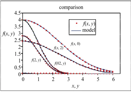
4. PROBLEM 3
For testing the above formulation several problems were considered. Here only one of them is presented. The data for this problem are obtained from the Eq.32.
] 3 , 0 [ ] 6 , 0 [ , , 4 ) ,
(x y e(0.0867 20.5 2) x y
z x y
(32) The domain of problem consists of 9 elements and 16 nodes. The elements are uniform where hi2 and
1 i
k . The above formulations were applied to to the governing data. Figure 3 shows the interpolation curves along x = 0, x = 2, y = 0 and y = 2. As it can be seen the 2-D model presents a close relationship to the relating set of data.
5. THE RESULTS AND CONCLUSIONS
In this research two models for 1-D and 2-D interpola-tions were presented. The models are easy and straight-forward to handle. Therefore; it can be applied for prob-lems having huge data. It has the advantage of less computational efforts respect to the cubic spline, Bezier and B-spline methods especially for 2-D problems. The continuity for each segment is C1 therefore; this is suffi-cient for many problems such as calculation of surfaces and volumes of nonuniform bodies. It is recommended to compare the 2-D model with Bezier and B-spine methods respect to the fitness and accuracy.
comparison
x, y
0
1 2 3 4 5 6 4.5 4 3.5 3 2.5 2 1.5 1 0.5 0
f(x, y)
f(x, y) model
f(x, 0)
f(x, 2)
f(2, y)
[image:4.595.309.538.542.704.2]f(02, y)
REFERENCES
[1] Salmon, D. (2006) Curves and surfaces for computer graphics. Springer, New York.
[2] Saxena, A. and Sahay, B. (2005) Computer aided engi-neering design. Springer, Anamaya Publisher, New Delhi. [3] Conte, S.D. and de Boor, C. (1981) Elementary
numeri-cal analysis, an algorithm approach. Kin Keong Printing Co. Pte. Ltd., Singapore.
[4] Burden, R. and Fairs, D. (1989) Numerical analysis. PWS-Kent Publishing Company, Boston.
[5] March, D. (2005) Applied geometry for compute graph-ics and CAD. 2nd Edition, Springer-Verlag, New York. [6] Todd, D.K. (1959) Groundwater hydrology. John Wily &