Abstract— This paper presents the initial results of a study aimed at improving the method by which the vibrations produced by transport vehicles are characterised and simulated. More specifically, this paper focuses on the rigid body vibrations generated by road transport vehicles in the context of distribution of packaged goods and produce. The research uses a variety of vibration data, collected from various vehicle types and routes in Spain and Australia with high-capacity vibration recorders. Vehicles used range from small transport vehicles to large truck-trailers with both airbags and steel spring suspensions while the routes travelled include suburban streets, main roads and motorways. The paper discusses the significance and limitations of the average power spectral density (PSD) and explains why the average PSD is not always adequate as the sole descriptor of road vehicle vibrations as the process generally tends to be non-stationary and non-Gaussian. The paper adopts an alternative analysis method, based on the statistical distribution of the moving root-mean-square (RMS) vibrations, as a supplementary indicator of overall ride quality. The measured data was used to compute the statistical distribution of each vibration record, the shape of which was compared for the entire set of records. The suitability of various mathematical models, based on the Weibull and Rayleigh distributions were investigated for describing the probability distribution function (PDF) of road vehicle vibration RMS time history. The paper proposes a single mathematical model that can accurately describe the statistical character of the random vibrations generated by road vehicles in general. It shows that the model can also effectively describe the statistical parameters of the process namely the mean, median, standard deviation, skewness and kurtosis.
Index Terms— Random vibrations, RMS distribution,
Weibull distribution.
I. INTRODUCTION
In order to develop optimum packaging it is important that engineers are not only aware, but have a thorough understanding of the expected mechanical hazards to which packages are subjected during shipping and handling. This information allows them to engineer the optimum amount of
M.A. Garcia-Romeu Martinez is with ITENE, Technological Institute of Packaging, Transportation and Logistics. Polígono Industrial D’Obradors, C/Soguers 2, 46110 Godella – Valencia, Spain. [email protected]
V. Rouillard is with Victoria University, Melbourne Australia PO Box 14428 MCMC, Melbourne 8001, Australia. [email protected]
V. Cloquell Ballester is with Valencia University of Technology, Spain. Camino de Vera s/n, 46021, Valencia, Spain. [email protected]
protective packaging needed to suitably protect the consignment against the risk of damage. To assist designers in reducing cost, either by avoiding wasting packaging materials due to over-packaging or avoiding damage due to under-packaging, distribution vibrations need to be simulated in the laboratory in order to test and validate protective package designs. Because verification of design by trial shipments have been shown to be both impractical and inadequate [1], performance testing of packaging systems in the laboratory has become increasingly the more adopted tool in the optimisation of package designs. Testing of package designs under controlled laboratory conditions usually involves the simulation of vibrations expected to be encountered during transportation. Assumptions regarding the nature and level of vibrations are sometimes adopted and make it difficult to optimise protective packaging without experimental verification. These unsophisticated and approximate simulation methodologies promote the adoption of a conservative approach to packaging design which, in many cases, lead to over packaging.
Vibrations that occur in vehicles during transportation are complex and play a significant role in the level of damage experienced by products during shipment. Vehicle vibrations have a random nature and their character and level is dependent on the type of vehicle, suspension type, payload, vehicle speed and road condition. Because of these variabilities, it is not always possible to represent transport vibrations with a simple function such as the power spectral density (PSD) function. With the advent of sophisticated vibration recorders in the past decade, packaging engineers have been able to measure and analyze increasing volumes of vibrations that occur in commercial shipments. Recently, numerous studies have been undertaken with the aim of measuring and evaluating the vibrations in various distribution environments around the globe and using particular vehicle types to enable packaging engineers to develop packaging solutions to meet world-wide distribution challenges [2][3][4][5][6]. The main purpose of these exercised was to generate effective laboratory test schedules for evaluating the performance of package systems when subjected to vehicle vibrations during distribution. Unfortunately, the prevailing trend is to characterise these complex vibrations with a single function namely, the average power spectral density (PSD).
A Model for the Statistical Distribution of Road
Vehicle Vibrations
-15 -10 -5 0 5 10 15
0 30 60 90 120 150 180 210 240 270 300 330
event number
a(
m/
s
2)
-6 -4 -2 0 2 4 6
cr
es
t fa
cto
r
[image:2.595.73.516.87.232.2]RMS Crest Factor
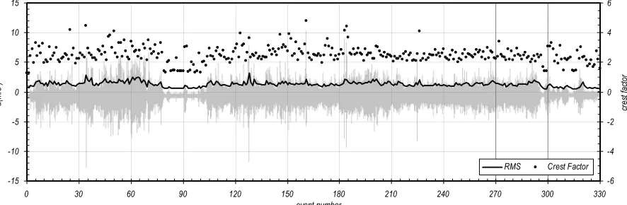
Figure 1. Typical road vehicle vibration record along with the RMS and crest factor time histories
The now well-established and widely adopted procedure for the laboratory simulation of vehicle vibrations is to synthesize random vibrations from the average PSD of measured vibration data (which is assumed to wholly describe the transport environment) using random vibration controllers. These controllers synthesize normally-distributed vibrations by continually computing the Inverse Fourier Transform of the PSD coupled with a uniformly distributed random phase array. Unfortunately, by virtue of the fact that these systems use solely the average PSD to synthesize a normally-distributed random signal, the simulated vibrations turn out to be stationary hence not capable of emulating the excursions in vibration amplitude which are found to occur in the field. One interesting characteristic of road vehicle vibrations is that the shape of the PSD remains largely unchanged for the duration of each transport event [6]. In effect, the non-stationarity of the process is manifested through fluctuations in RMS level [7]. Most vibration controllers can be programmed so that the RMS level of the synthesised random signal is made to vary as a function of time. However, there is no established technique to determine how this modulation of amplitude should be implemented.
The main objective of this paper is to establish whether a single mathematical model can be used to describe the statistical distribution of the moving RMS of vibrations generated by road vehicles in general, and whether the model can be used to characterise the overall ride quality as well as be of use in determining laboratory test schedules that include the generation of random vibrations of varying RMS levels.
II. MODELLING THE RMS DISTRIBUTION
Rouillard & Sek [8], studied the non-stationary behaviour of road vehicle vibrations and proposed a statistical model for characterising what they term the “vibration intensity”. Their model is a modified version of the Rayleigh distribution that includes an exponent parameter and a scale parameter. Their model applied to the vibration intensity which can only be computed by an elaborated algorithm based on the Hilbert transform. Further work aimed at using the RMS distribution
of vehicle vibrations to design laboratory tests schedules was undertaken by Rouillard & Sek [7]. This work shows how more realistic vibrations can be synthesized by recognizing that road vehicle vibrations are non-stationary and by making use of the RMS distribution. One of the most elementary approaches to characterising non-stationarities is to compute the RMS (or mean-square) of the vibration record over relatively short segments [9]. The length of the segments and the incremental step for computing the moving RMS are critical to the analysis. The moving RMS of a function x(t) can be written as:
( )
i w 2( )
i
j i 1
ˆx t x j for i 0, ,2 ,3 ...N
n δ δ δ δ
+
=
=
∑
= (1)Where w is the segment length, δ is the incremental step and N is the total number of segments in the sample.
The effects of the window width and the incremental step (overlap) on the moving RMS of non-stationary vibration signals have been illustrated by Rouillard [10]. It shows that care must be taken in selecting the parameters for computing the RMS time history of non-stationary signals.
In order to validate the proposed model, a number of sample vibration records were collected from a wide range of vehicles and routes. The vibration data were collected using self-contained data recorders (Saver® by Lansmont) configured to record vibrations for predetermined sub-record lengths of 8 seconds at a sampling rate of 1024 Hz. The recorders were configured to initiate recording at specific periods varying from 9 seconds to one minute. A total of thirteen measurements were undertaken using various vehicles including small utility, vans, rigid trucks and semi-trailers with various suspension types and payloads. Routes included poorly maintained local roads, country roads, urban roads, and highways located in Victoria, Australia and Spain as shown in Table 1. The RMS time history of each vibration record was computed using (1) with
w = 8 seconds and no overlap (δ = w + 1/fs, where fs =
includes a plot the moving crest factor which indicates the non-stationary character of the process; for a Gaussian process of 8192 samples, the likelihood that the crest factor exceeds 3.65 is 0.012%. This is a strong indication that the data recorded are non-Gaussian and non-stationary [10].
Table 1. Summary of measured vibration record parameters.
Record ID Vehicle type & load Country Route Type
DATA A Utility vehicle (1 Tonne cap.). Load: < 5% cap.
Australia Suburban streets
DATA B Prime mover + Semi trailer (Air ride susp.). Load: 90% cap.
Australia Country roads
DATA C Transport van (700 kg cap.). Load:
60% cap. Australia Suburban streets DATA D Transport van (700 kg cap.). Load:
60% cap. Australia Main hwy suburban DATA E Transport van (700 kg cap.). Load:
60% cap. Australia Motorway DATA F Prime mover + Semi trailer (Leaf
spring susp.). Load: < 5% cap. Australia Country roads DATA G Tipper truck (16 Tonnes cap., Air
ride susp.). Load: 25% capacity. Australia Country roads DATA H Small flat bet truck (1 Tonne cap.,
Leaf spring susp.). Load <5% cap. Australia Suburban streets DATA J Flat bed truck (5 Tonnes cap., Leaf
spring susp.). Load >95% cap.
Australia Country roads
DATA K Sedan car. Load: 1 passenger Australia Suburban streets DATA L Prime mover + Semi trailer (Air ride
susp.). Load: 60% cap. Spain Motorway DATA M Prime mover + Semi trailer (Air ride
susp.). Load: 20% cap. Spain Motorway DATA N Prime mover + Semi trailer (Leaf
spring susp.). Load: 10% cap. Spain Motorway DATA O Prime mover + Semi trailer (Leaf
spring susp.). Load: < 1% cap. Spain Motorway The Probability Density Function (PDF) of the RMS time history of each of the thirteen vibration records was computed with the aim of developing a generic mathematical model that can be used to characterise the statistical characteristics of the process regardless of vehicle type, payload or route.
A range of statistical distributions were studied and a model given in (3) was developed, based on the three-parameter Weibull distribution given in (2).
( )
0 1 00
x x x x
P x e x x
γ γ
α γ
α α
−
− −
−
= ⋅ ∀ ≥
(2)
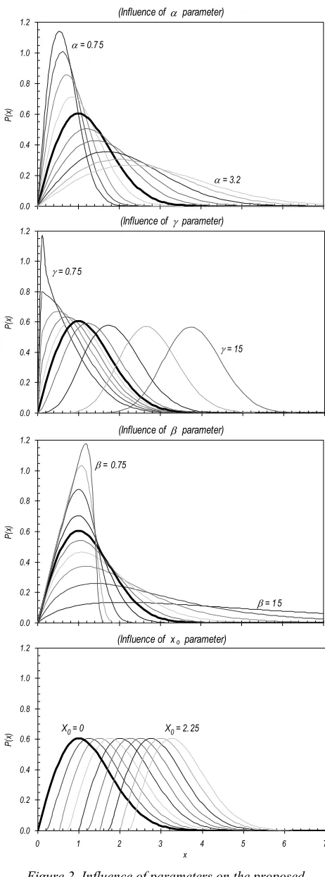
The proposed modified Weibull distribution model was developed to afford additional control over various aspects of the shape of the distribution function. It includes an exponent parameter, β, which enables the control of the slope of the right-hand tail of the distribution and increases the scope of the model for characterising a wider range of distribution functions. The model, given in (3), was found to be generic enough to be able to produce a range of well-known distributions for which the parameters are given in Table 2.
( )
]
]
[
[
0
0 1
0
0 1
0
0 , //
// ,
,
i i
x x
i i
i
x x x x
P x x x
e x x x x
x x
where
β γ
α
β γ
β ρ
α
β ρ
α α
−
− −
−
∀ ∈ −∞ ≥
= −
⋅ ⋅ ∀ ∈ ≥ +∞
−
= ⋅ Γ
(3)
Where x is the moving RMS, α, β, γ and x0 are the modified
Weibull parameters and xi is the left hand domain limit.
(Influence of α parameter)
0.0 0.2 0.4 0.6 0.8 1.0 1.2
0 1 2 3 4 5 6 7
x
P(
x)
(Influence of γ parameter)
0.0 0.2 0.4 0.6 0.8 1.0 1.2
0 1 2 3 4 5 6 7
x
P(
x)
α= 0.75
α= 3.2
γ= 0.75
γ= 15
(Influence of β parameter)
0.0 0.2 0.4 0.6 0.8 1.0 1.2
P(
x)
(Influence of xo parameter)
0.0 0.2 0.4 0.6 0.8 1.0 1.2
0 1 2 3 4 5 6 7
x
P(
x)
β= 0.75
β= 15
X0= 0 X0= 2.25
[image:3.595.47.277.176.376.2]Table 2. Parameters values for typical distributions.
The single-parameter statistics for the model, namely, the mean, µ, the median, mdn, the standard deviation, σ, the skewness, ν (Sk) and the kurtosis, Kt, were derived and are given as:
[ ]1
0
x
µ= + ⋅ Ψα (4)
0 1 0
, ,
2
i
mdn x β x x β
γ γ
β α β α
− −
Γ = ⋅Γ
(5)
( )
( )
[ ] 2 2 22 2 2
0 0
2
E x
where E x x x
σ µ
α µ
= −
= Ψ + −
(6)
( )
( )
( )
[ ] [ ]3 2 3
3
3 2
3 3 2 2 3
0 0 0
1
3 2
3 3 2
Sk E x E x
where E x x x x
ν µ µ
σ
α α µ
= = − ⋅ −
= Ψ + Ψ + −
(7)
( )
( )
( )
( )
[ ] [ ] [ ][ ]
4 3 2 2 4 4
4 3 2
4 4 3 2 2 3 4
0 0 0 0
1
4 6 3
4 6 4 3 ,
,
,
j i o
j
i o
Kt E x E x E x
where E x x x x x
x x and x x β γ β β γ β
µ µ µ
σ
α α α µ
α
α +
= − ⋅ + ⋅ −
= Ψ + Ψ + Ψ + −
−
Γ
Ψ =
−
Γ
(8)
In the case of the RMS distribution, the left hand domain limit, xi, was chosen as greater than zero since the RMS time
history is, by definition, always positive. For the purpose of this study, in which only rigid body vibrations are of interest,
xi = xo. This has the effect of discounting the sustained,
residual low level vibrations that are not caused by road – pavement interactions [10]. Therefore (3) can be written as follows, to characterise the moving RMS PDF of road vehicle vibrations:
( )
]
[
[
[
0 0 1 0 0 0 , , x x x xP x x x
e x x
β γ α γ β β α α − − − ∀ ∈ −∞ = − ⋅ ∀ ∈ +∞
⋅Γ
(9)
The influence of each of the four parameters on the shape of the distribution function are illustrated in Fig. 2 which shows that each parameter alters different aspects of the distribution shape.
Further analyses, undertaken to investigate the cross-correlation between the parameters, showed that there is no significant inter-parameter dependence.
_ ?
error error min<
Random initial conditions
1 (1) 1 (1) 2 (1) 0 1 (1)
i i i oi rand rand rand x rand α ε β ε γ ε = + ⋅ = + ⋅ = + ⋅ = + ⋅
Matlab function to fit an equation to a data by least squares optimisation
[ ]
(' _ ',' , , ,o', '[ ]')
Inline Eq Model α β γx Data to fit
[Data to fit] Least squares fit[ ] , , ,xo
α β γ S
0
, , 0and x 0 ?
α β γ > ≥
Calculate statistic parameters for the model
1 2 3 4 5 _ _ _ _ _
model_sp model mean model_sp model median model_sp model std model_sp model Sk model_sp model Kt
= = = = =
Calculate the error of the statistic parameters
( ) 5 1 2 5 1 1 _ 5 _ _ 5 _ _ i i i i i i model_sp data_sp mean error data_sp
model_sp mean error std error
error mean error std error
= = − = ⋅ − = = + ∑ ∑ n=n+1 n=0 max_iter k, ε, error_min
Best fit
[α β γ, , ,xo]
?
n max_iter< _ _
0
error min k error min n = ⋅ = E False True False True True _ ?
error error min<
Random initial conditions
1 (1) 1 (1) 2 (1) 0 1 (1)
i i i oi rand rand rand x rand α ε β ε γ ε = + ⋅ = + ⋅ = + ⋅ = + ⋅
Matlab function to fit an equation to a data by least squares optimisation
[ ]
(' _ ',' , , ,o', '[ ]')
Inline Eq Model α β γx Data to fit
[Data to fit] Least squares fit[ ] , , ,xo
α β γ S
0
, , 0and x 0 ?
α β γ > ≥
Calculate statistic parameters for the model
1 2 3 4 5 _ _ _ _ _
model_sp model mean model_sp model median model_sp model std model_sp model Sk model_sp model Kt
= = = = =
Calculate the error of the statistic parameters
( ) 5 1 2 5 1 1 _ 5 _ _ 5 _ _ i i i i i i model_sp data_sp mean error data_sp
model_sp mean error std error
error mean error std error
= = − = ⋅ − = = + ∑ ∑ n=n+1 n=0 max_iter k, ε, error_min
Best fit
[α β γ, , ,xo]
?
n max_iter< _ _
0
[image:4.595.77.503.291.738.2]error min k error min n = ⋅ = E False True False True True
III. RESULTS
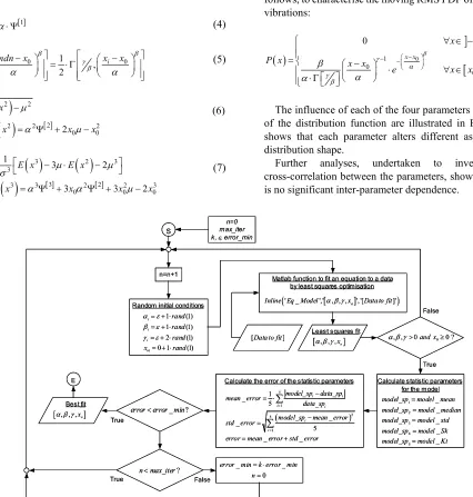
A computer program (coded in Matlab®) was developed to determine the optimum parameter values that yield the best fit for the proposed model with respect to the PDF of measured vibration data. Results using the sum-of-squared error (least squares) optimisation were found to produce unstable results. This was attributed to the relatively large number (four) of independent parameters which was found to achieve least square errors for several combinations of parameter values. In order to address this difficulty, code was modified (Fig. 3) to include optimisation based on the mean and standard deviation of the errors between the fitted and measured data for five statistical parameters namely the mean, median, standard deviation, skewness, and kurtosis.
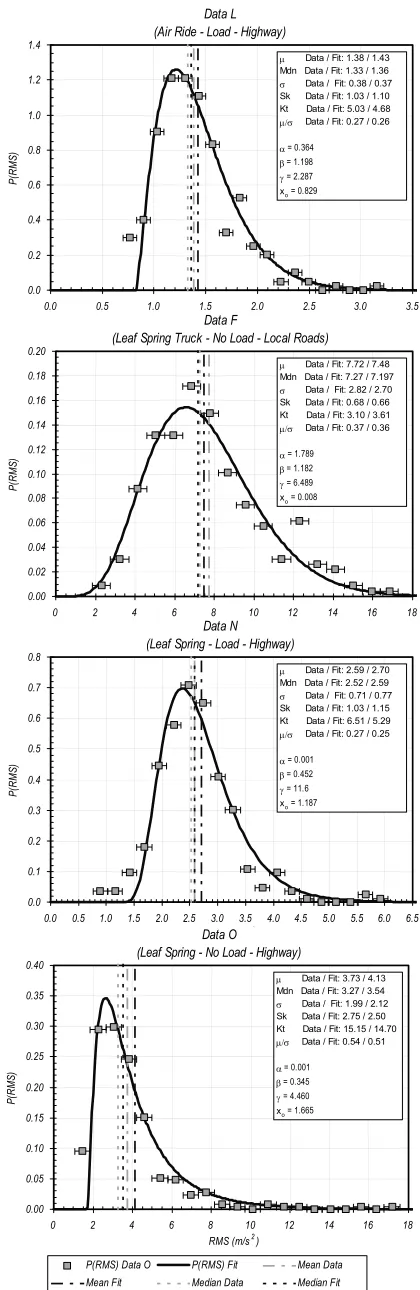
This curve fitting algorithm was used to subject the proposed four-parameter modified Weibull model to validation tests using all thirteen vibration records (Table 1) and was found to offer good agreement as shown in Fig. 4 which shows four typical examples.
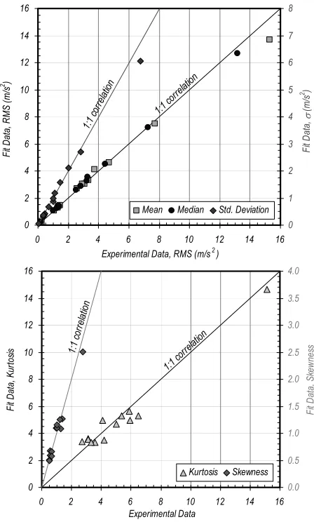
The goodness of fit between the distribution of the measured data and the model are best revealed graphically as shown in Fig. 5 which shows plots of the main statistical parameters for all thirteen cases. It can be seen that very good agreement is achieved (R2 = 0.99) for the first and
second order statistics (mean, median and standard deviation) while reasonably good agreement is achieved (R2
= 0.96) for the third and fourth order statistics, represented here by the skewness and Kurtosis.
The analysis of all thirteen vibration records show that the model is capable of representing RMS distributions consisting of various values of kurtosis, skewness and standard deviations as shown in Fig. 5.
IV. CONCLUSIONS
This paper has presented the initial results of a study aimed at improving the method by which the rigid body vibrations produced by road transport vehicles are characterised. Vibration data, collected from various vehicle types and routes in Spain and Australia, was used to develop and validate a mathematical model, based on the Weibull distribution, to describe the probability density function of the moving RMS time histories of the process. The paper has addressed the limitations of the average power spectral density (PSD) and explains why the average PSD is not always adequate as the sole descriptor of road vehicle vibrations as the process generally tends to be non-stationary and non-Gaussian.
Data L (Air Ride - Load - Highway)
0.0 0.2 0.4 0.6 0.8 1.0 1.2 1.4
0.0 0.5 1.0 1.5 2.0 2.5 3.0 3.5
RMS (m/s2)
P(
R
M
S)
P(RMS) Data L P(RMS) Fit Mean Data
Mean Fit Median Data Median Fit
µ Data / Fit: 1.38 / 1.43 Mdn Data / Fit: 1.33 / 1.36 σ Data / Fit: 0.38 / 0.37 Sk Data / Fit: 1.03 / 1.10 Kt Data / Fit: 5.03 / 4.68 µ/σ Data / Fit: 0.27 / 0.26
α = 0.364
β = 1.198
γ = 2.287
xo= 0.829
Data F
(Leaf Spring Truck - No Load - Local Roads)
0.00 0.02 0.04 0.06 0.08 0.10 0.12 0.14 0.16 0.18 0.20
0 2 4 6 8 10 12 14 16 18
RMS (m/s2)
P(
R
M
S)
P(RMS) Data F P(RMS) Fit Mean Data
Mean Fit Median Data Median Fit
µ Data / Fit: 7.72 / 7.48 Mdn Data / Fit: 7.27 / 7.197 σ Data / Fit: 2.82 / 2.70 Sk Data / Fit: 0.68 / 0.66 Kt Data / Fit: 3.10 / 3.61 µ/σ Data / Fit: 0.37 / 0.36
α = 1.789
β = 1.182
γ = 6.489
xo= 0.008
Data N (Leaf Spring - Load - Highway)
0.0 0.1 0.2 0.3 0.4 0.5 0.6 0.7 0.8
0.0 0.5 1.0 1.5 2.0 2.5 3.0 3.5 4.0 4.5 5.0 5.5 6.0 6.5
RMS (m/s2)
P(
R
M
S)
P(RMS) Data N P(RMS) Fit Mean Data
Mean Fit Median Data Median Fit
µ Data / Fit: 2.59 / 2.70 Mdn Data / Fit: 2.52 / 2.59 σ Data / Fit: 0.71 / 0.77 Sk Data / Fit: 1.03 / 1.15 Kt Data / Fit: 6.51 / 5.29 µ/σ Data / Fit: 0.27 / 0.25
α = 0.001
β = 0.452
γ = 11.6
xo= 1.187
Data O (Leaf Spring - No Load - Highway)
0.00 0.05 0.10 0.15 0.20 0.25 0.30 0.35 0.40
0 2 4 6 8 10 12 14 16 18
RMS (m/s2)
P(
R
M
S)
P(RMS) Data O P(RMS) Fit Mean Data
Mean Fit Median Data Median Fit
µ Data / Fit: 3.73 / 4.13 Mdn Data / Fit: 3.27 / 3.54 σ Data / Fit: 1.99 / 2.12 Sk Data / Fit: 2.75 / 2.50 Kt Data / Fit: 15.15 / 14.70 µ/σ Data / Fit: 0.54 / 0.51
α = 0.001
β = 0.345
γ = 4.460
xo= 1.665
Data L (Air Ride - Load - Highway)
0.0 0.2 0.4 0.6 0.8 1.0 1.2 1.4
0.0 0.5 1.0 1.5 2.0 2.5 3.0 3.5
RMS (m/s2)
P(
R
M
S)
P(RMS) Data L P(RMS) Fit Mean Data
Mean Fit Median Data Median Fit
µ Data / Fit: 1.38 / 1.43 Mdn Data / Fit: 1.33 / 1.36 σ Data / Fit: 0.38 / 0.37 Sk Data / Fit: 1.03 / 1.10 Kt Data / Fit: 5.03 / 4.68 µ/σ Data / Fit: 0.27 / 0.26
α = 0.364
β = 1.198
γ = 2.287
xo= 0.829
Data F
(Leaf Spring Truck - No Load - Local Roads)
0.00 0.02 0.04 0.06 0.08 0.10 0.12 0.14 0.16 0.18 0.20
0 2 4 6 8 10 12 14 16 18
RMS (m/s2)
P(
R
M
S)
P(RMS) Data F P(RMS) Fit Mean Data
Mean Fit Median Data Median Fit
µ Data / Fit: 7.72 / 7.48 Mdn Data / Fit: 7.27 / 7.197 σ Data / Fit: 2.82 / 2.70 Sk Data / Fit: 0.68 / 0.66 Kt Data / Fit: 3.10 / 3.61 µ/σ Data / Fit: 0.37 / 0.36
α = 1.789
β = 1.182
γ = 6.489
xo= 0.008
Data N (Leaf Spring - Load - Highway)
0.0 0.1 0.2 0.3 0.4 0.5 0.6 0.7 0.8
0.0 0.5 1.0 1.5 2.0 2.5 3.0 3.5 4.0 4.5 5.0 5.5 6.0 6.5
RMS (m/s2)
P(
R
M
S)
P(RMS) Data N P(RMS) Fit Mean Data
Mean Fit Median Data Median Fit
µ Data / Fit: 2.59 / 2.70 Mdn Data / Fit: 2.52 / 2.59 σ Data / Fit: 0.71 / 0.77 Sk Data / Fit: 1.03 / 1.15 Kt Data / Fit: 6.51 / 5.29 µ/σ Data / Fit: 0.27 / 0.25
α = 0.001
β = 0.452
γ = 11.6
xo= 1.187
Data O (Leaf Spring - No Load - Highway)
0.00 0.05 0.10 0.15 0.20 0.25 0.30 0.35 0.40
0 2 4 6 8 10 12 14 16 18
RMS (m/s2)
P(
R
M
S)
P(RMS) Data O P(RMS) Fit Mean Data
Mean Fit Median Data Median Fit
µ Data / Fit: 3.73 / 4.13 Mdn Data / Fit: 3.27 / 3.54 σ Data / Fit: 1.99 / 2.12 Sk Data / Fit: 2.75 / 2.50 Kt Data / Fit: 15.15 / 14.70 µ/σ Data / Fit: 0.54 / 0.51
α = 0.001
β = 0.345
γ = 4.460
[image:5.595.326.536.82.727.2]xo= 1.665
The paper adopts an alternative analysis method, based on the statistical distribution of the moving root-mean-square (RMS) vibrations, as a supplementary indicator of overall ride quality. The paper proposes a single mathematical model that can accurately describe the statistical character of the random vibrations generated by road vehicles in general.
0 2 4 6 8 10 12 14 16
0 2 4 6 8 10 12 14 16
Experimental Data
Fi
t D
ata,
K
ur
tos
is
0.0 0.5 1.0 1.5 2.0 2.5 3.0 3.5 4.0
Fi
t D
ata, Sk
ew
nes
s
Kurtosis Skewness
1:1 c orre
latio n
1:1 co rrelati
on
0 2 4 6 8 10 12 14 16
0 2 4 6 8 10 12 14 16
Experimental Data, RMS (m/s2)
Fi
t D
ata, R
M
S (
m
/s
2 )
0 1 2 3 4 5 6 7 8
Fi
t D
ata,
σ
(m
/s
2 )
Mean Median Std. Deviation
1:1 corre
lation
1:1 co
rrelatio
n
0 2 4 6 8 10 12 14 16
0 2 4 6 8 10 12 14 16
Experimental Data
Fi
t D
ata,
K
ur
tos
is
0.0 0.5 1.0 1.5 2.0 2.5 3.0 3.5 4.0
Fi
t D
ata, Sk
ew
nes
s
Kurtosis Skewness
1:1 c orre
latio n
1:1 co rrelati
on
0 2 4 6 8 10 12 14 16
0 2 4 6 8 10 12 14 16
Experimental Data
Fi
t D
ata,
K
ur
tos
is
0.0 0.5 1.0 1.5 2.0 2.5 3.0 3.5 4.0
Fi
t D
ata, Sk
ew
nes
s
Kurtosis Skewness
1:1 c orre
latio n
1:1 co rrelati
on
0 2 4 6 8 10 12 14 16
0 2 4 6 8 10 12 14 16
Experimental Data, RMS (m/s2)
Fi
t D
ata, R
M
S (
m
/s
2 )
0 1 2 3 4 5 6 7 8
Fi
t D
ata,
σ
(m
/s
2 )
Mean Median Std. Deviation
1:1 corre
lation
1:1 co
rrelatio
n
0 2 4 6 8 10 12 14 16
0 2 4 6 8 10 12 14 16
Experimental Data, RMS (m/s2)
Fi
t D
ata, R
M
S (
m
/s
2 )
0 1 2 3 4 5 6 7 8
Fi
t D
ata,
σ
(m
/s
2 )
Mean Median Std. Deviation
1:1 corre
lation
1:1 co
rrelatio
[image:6.595.49.273.165.537.2]n
Figure 5. Goodness of fit plots for the main statistical parameters.
The proposed modified Weibull distribution model was developed to afford additional control over various aspects of the shape of the distribution function. The model was found to be generic enough to be able to produce a range of well-known distributions. Curve fitting results using the sum-of-squared error (least squares) optimisation were found to produce unstable results which required inclusion of the mean, median, standard deviation, skewness, and kurtosis in the optimisation algorithm. Validation tests using all thirteen sample vibration records and was found to offer good agreement in general. The paper also shows how the model is capable of accurately describing the statistical parameters of the process namely the mean, median, standard deviation, skewness and kurtosis.
This result is relevant not only for the characterisation of ride quality but also for the accurate synthesis of road vehicle vibrations in the laboratory. The results can be used to assist in developing a novel method for simulating non-stationary (modulated) vibration in the laboratory. The RMS distribution function can be used to create an RMS level schedule that will enable the synthesis of random vibrations with varying RMS level to better represent the road transport vibration process.
REFERENCES
[1] M. A. Sek, “Optimisation of Packaging Design Through an Integrated Approach to the Measurement and Laboratory Simulation of Transportation Hazards”, Proceedings of the 12th International Conference on Packaging, International Association of Packaging Research Institutes, Warsaw, Poland, 2001
[2] S. P. Singh, E. Joneson and J. Singh, “Measurement and analysis of US truck vibration for leaf spring and air ride suspensions, and development of tests to simulate these conditions”, Journal of Packaging Technology and Science, 2006, 19: 309-323
[3] S. P. Singh and J. Marcondes, “Vibration levels in comercial truck shipments as a function of suspension and payload”, Journal of Testing and Evaluation, 1992, Vol 20, No. 6, 466-469
[4] C. Pierce, S. P. Singh and G. A. Burgess, “Comparison of leaf spring to air cushion trailer suspensions in the transportation environment”, Journal of Packaging Technology and Science, 1992, Vol 5, 11-15 [5] S. P. Singh, J. Antle and G. A. Burgess, “Comparison between lateral,
longitudinal and vertical vibration levels in commercial truck shipments”, Journal of Packaging Technology and Science, 1992, Vol. 5, 71-75
[6] M. A. Garcia-Romeu-Martinez and S.P. Singh, “Developing Vibration Simulation Methods for Truck Transport in Spain as a Function of Payload, Suspension and Truck Speed”, Proceedings of the 15th International IAPRI World Conference on Packaging, Tokyo, Japan, 2006, 19-25
[7] V. Rouillard. and M. A. Sek, “Generating road vibration test schedules from pavement profiles for packaging optimization”, Proceedings of the 21st IAPRI Symposium on Packaging, Valencia, Spain, 2003 [8] V. Rouillard and M. A. Sek, “Statistical modelling of predicted non-
stationary vehicle vibrations”, International Journal of Packaging Technology and Science, 2002, Vol 15 (2), pp 93-101
[9] J. S. Bendat and A. G. Piersol, “Random data analysis and measurement procedures”, John Wiley and Sons, New York, 1986 [10] V. Rouillard, “On the Laboratory Synthesis of Non-stationary Road