Interactive Random Fuzzy Two-Level Programming through Possibility-based Fractile Criterion Optimality

(1)

Interactive Random Fuzzy Two-Level

Programming through Possibility-based Fractile

Criterion Optimality

Hideki Katagiri, Keiichi Niwa, Daiji Kubo, Takashi Hasuike

∗

Abstract—This paper considers two-level linear pro-gramming problems where each coeﬃcient of the ob-jective functions is expressed by a random fuzzy vari-able. A new decision making model is proposed in order to maximize both of possibility and probabil-ity with respect to the objective function value. Af-ter the original random fuzzy two-level programming problem is reduced to a deterministic one through the proposed model, interactive programming to derive a satisfactory solution for the decision maker at the up-per level in consideration of the cooup-perative relation between decision makers is presented.

Keywords: random fuzzy variable, cooperative two-level programming, possibility measure, fractile criterion, interactive algorithm

1 Introduction

In the real world, we often encounter situations where there are two decision makers in an organization with a hierarchical structure, and they make decisions in turn or at the same time so as to optimize their objective func-tions. When we formulate two-level programming prob-lems which closely represents such a real-world decision situation under hierarchical structure, it is often the case that the objective functions and the constraints involve many uncertain parameters.

From a probabilistic point of view, two-level or multi-level programming with random variable coeﬃcients was developed by Nishizaki et al. [13] and Roghanian et al. [15]. Considering the vague nature of the DM’s judg-ments in two-level linear programming, a fuzzy program-ming approach was ﬁrst presented by Shih et al. [17] and further studied by Sakawa et al. [16].

Although these studies focused on either fuzziness or ran-domness included in two-level decision making situations, it is important to realize that simultaneous considerations of both fuzziness and randomness would be required in order to to utilize two-level programming for resolution

∗_{Corresponding} _Author: _Hideki _Katagiri ([email protected]), Graduate School of Engineering, Hiroshima University, 1-4-1 Kagamiyama, Higashi-Hiroshima City, Hiroshima, 739-8527 Japan

of conflict in decision making problems in real-world de-centralized organizations. For example, when estimating the values of coefficients in problems as random variables, their mean values are estimated as constants using sta-tistical analysis. However, in more realistic cases, the direct use of mean values estimated based on past data may not be appropriate for decision making for future planning. For dealing with such decision making situa-tions, a random fuzzy variable, first defined by Liu [11], draws attention as a new tool for decision making under random fuzzy environments [5, 6, 11, 19].

In general, two-level programming models are classiﬁed into two categories; one is a noncooperative model em-ploying the solution concept of Stackelberg equilibrium, and the other is a cooperative model for situations where there exists communication and some cooperative rela-tionship among the decision makers in such as decentral-ized large ﬁrms with divisional independence.

In this paper, we focus on the cooperative case and con-sider solution methods for decision making problems in hierarchical organizations under random fuzzy environ-ments. A new decision making model is proposed based on the fusion of stochastic programming model and pos-sibilistic programming model in order to maximize both of possibility and probability with respect to the attained objective function value. After showing that the random fuzzy two-level programming problem can be reduced to a deterministic one through the proposed model called possibility-based fractile model, we present an interac-tive algorithm to derive a satisfactory solution for the decision maker at the upper level in consideration of the cooperative relation between decision makers.

2 Random fuzzy two-level linear

pro-gramming problems

A random fuzzy variable, ﬁrst introduced by Liu [11], is deﬁned follows:

(2)

n-dimensional random fuzzy vectorn= (ξ1, ξ2, . . . , ξn)is

an n-tuple ofrandom fuzzy variablesξ= (ξ1, ξ2, . . . , ξn).

Intuitively speaking, a random fuzzy variable is an ex-tended mathematical concept of random variable in the sense that it is defined as a fuzzy set defined on a uni-versal set of random variables. For instance, the random variables with fuzzy mean values are represented with random fuzzy variables. It should be noted here that a random fuzzy variable is not different from a fuzzy ran-dom variable [4, 9, 10, 12], which is used to deal with the ambiguity of realized values of random variables, not fo-cusing on the ambiguity of parameters charactezing ran-dom variables like ranran-dom fuzzy variables.

In this paper, we deal with two-level linear programming problems involving random fuzzy variable coeﬃcients in objective functions formulated as:

minimize

for DM1 z1(x1,x2) =

¯ ˜

C11x1+C¯˜12x2

minimize

for DM2 z2(x1,x2) =

¯ ˜

C21x1+C¯˜22x2

subject to A1x1+A2x2≤b

x1≥0, x2≥0

          

. (1)

It should be emphasized here that randomness and fuzzi-ness of the coeﬃcients are denoted by the “dash above” and “wave above” i.e., “ ¯ ” and “ ˜ ”, respectively. In this formulation, x1 is an n1 dimensional decision

vari-able column vector for the DM at the upper level (DM1),

x2 is an n2 dimensional decision variable column vector

for the DM at the lower level (DM2), z1(x1,x2) is the

objective function for DM1 and z2(x1,x2) is the

objec-tive function for DM2. In (1), C¯˜lj, l = 1,2,j = 1,2 are vectors whose elementsC¯˜ljk,k= 1,2, . . . , nj are random fuzzy variables which are normal random variables with ambiguous mean values. In particular, we assume that the probability function of C¯˜ljk is formally represented with

fljk(z) = 1 √

2πσljk exp−

(z−_Mljk˜ )2 2σ2

ljk _, ₍₂₎

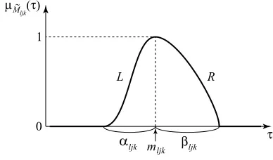
where ˜Mljkis anL-Rfuzzy number characterized by the following membership function (see Figure 1):

µM˜ljk(τ) =         

L

µ

mljk−τ

αljk

¶

(mljk≥τ)

R

µ

τ−mljk

βljk

¶

(mljk< τ).

(3)

FunctionsLandRare called reference functions or shape functions which are nonincreasing upper semi-continuous functions [0,∞)→[0,1].

[image:2.595.329.523.72.186.2]

Random fuzzy two-level linear programming problems formulated as (1) are often seen in actual decision making

Figure 1: Membership functionµ_M˜

ljk(·).

situations. For example, consider a supply chain plan-ning where the distribution center (DM1) and the pro-duction part (DM2) hope to minimize the distribution cost and the production cost, respectively. Since coeﬃ-cients of these objective functions are often aﬀected by the economic conditions varying at random, they can be regarded as random variables.

When C¯˜ljk is a random fuzzy variable characterized by

(2) and (3), the membership function of C¯˜j is expressed as

µ_C¯˜_ljk(¯γljk) = sup sljk

{µM˜ljk(sljk)|γ¯ljk∼N(sljk, σ

2

ljk)}, (4)

where ¯γljk∈Γ, and Γ is a universal set of normal random variables. Each membership function value µ_C¯˜_ljk(¯γj) is interpreted as a degree of possibility or compatibility that

¯˜

Cljk is equal to ¯γljk.

Then, applying the results shown by Liu [11], the objec-tive function C¯˜lx is deﬁned as a random fuzzy variable characterized by the following membership function:

µ¯_˜

Clx(¯ul)

△ = sup

¯

γl n

min

1≤k≤nj, j=1,2

µ_C¯_˜

ljk(¯γljk) ¯¯ ¯

¯ ul=

2

X

j=1

nj X

k=1

¯ γljkxjk

o

, ∀u¯l∈Yl, (5)

where ¯γ_l = (¯γl11, . . . ,γ¯l1n1,γ¯l21, . . . ,¯γl2n2) and Yl is

de-ﬁned by

Yl=

  

2

X

j=1

nj X

k=1

¯

γljkxjk¯¯¯¯γljk∈Γ,

 

, l= 1,2.

From (4) and (5), we obtain

µ_C¯˜

lx(¯ul)

= sup

sl ½

min

1≤k≤nj, j=1,2

(3)

¯

γljk∼N(sljk, σljk2 ), u¯l=

2

X

j=1

nj X

k=1

¯ γljkxjk

  

= sup

sl ½

min

1≤k≤nj, j=1,2

µ_M˜_ljk(sljk)¯¯¯

¯ ul∼N

 X2

j=1

nj X

k=1

sljkxjk,

2

X

j=1

nj X

k=1

σ2_ljkx2_jk

 

  (6)

wheresl= (sl11, . . . , sl1n1, s121, . . . , sl2n2).

Considering that the mean values of random variables are often ambiguous and estimated as fuzzy numbers using experts’ knowledge based on their experiences, the coef-ﬁcients are expressed by random fuzzy variables. Then, such a supply chain planning problem can be formulated as a two-level linear programming problem involving ran-dom fuzzy variable coeﬃcients like (1).

In stochastic programming, basic optimization criterion is to simply optimize the expectation of objective func-tion values or to decrease their ﬂuctuafunc-tion as little as possible from the viewpoint of stability. In contrast to these types of optimizing approaches, the fractile model or Kataoka’s model [8] has been proposed when the deci-sion maker wishes to optimize a permissible level under the guaranteed probability that the objective function value is better than or equal to the permissible level.

On the other hand, in fuzzy programming, possibilistic programming [7] is one of methodologies for decision mak-ing under existence of ambiguity of the coeﬃcients in ob-jective functions and constraints.

In this research, we consider a new random fuzzy two-level programming in order to simultaneously optimize both possibility and probability with the attained ob-jective function values of DMs, by extending both view-points of stochastic programming and possibilistic pro-gramming.

To begin with, let us express the probability

Pr

³

ω¯¯C˜¯l(ω)x≤fl

´

as a fuzzy set P˜l and deﬁne

the membership function of ˜P as follows:

µ_P˜_l(pl) = sup

¯

ul n

µ_C_˜¯

lx(¯ul) ¯¯

¯pl= Pr (ω|u¯l(ω)≤fl)

o

. (7)

From (6) and (7), we obtain

µP˜l(pl)

= sup

sl

min

1≤k≤nj, j=1,2 n

µ_M˜_ljk(sljk)¯¯¯pl= Pr (ω|u¯l(ω)≤fl),

¯ ul∼N

³X2

j=1

nj X

k=1

sljkxjk,

2

X

j=1

nj X

k=1

σ_ljk2 x2_jk

´o

.

[image:3.595.327.525.70.185.2]

Assuming that each of DMl, l= 1,2 has a goalGlfor the attained probability expressed as “ ˜Pl should be greater

Figure 2: Membership functionµl(·).

than or equal to some value ˆpl. Then, the possibility that ˜

Plsatisﬁes the goal Gl is expressed as

Π_P˜

l(Gl)

△ = sup

pl

{µ_P˜

l(pl)|pl≥pˆl}.

Then, as a new optimization model in two-level program-ming problems with random fuzzy variables, we consider the following possibility-based fractile model:

maximize

for DM1 µ1(f1)

maximize

for DM2 µ2(f2)

subject to ΠP˜1(G1)≥h1

Π_P˜

2(G2)≥h2

A1x1+A2x2≤b

x1≥0, x2≥0

                

(8)

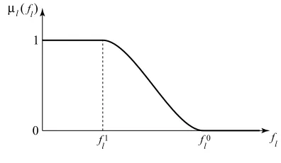
whereh1 andh2 are constants. Functionsµ1and µ2are

the membership functions of fuzzy goals for the aspiration levelsf1andf2, respectively, which reﬂects the vagueness

in human judgments for the aspiration levels (see Figure 2).

Then we can derive the following theorem:

Theorem 1 Let T denotes the distribution function of

N(0,1)andKpˆl

△

=T−1(ˆpl). Then,ΠP˜l(Gl)≥hlin

prob-lem (8) is equivalently transformed into

2

X

j=1

nj X

k=1

{mljk−L∗(hl)αljk}xjk+Kpˆl v u u tX2

j=1

nj X

k=1

σ_ljk2 x2_jk ≤fl

where L∗(hl) is a pseudo inverse function deﬁned as

L∗(hl) = sup{t|L(t)≥hl}.

Proof: The constraint Π_P˜_l(Gl)≥hl, l= 1,2 in problem (8) is equivalently transformed as follows:

Π_P˜_l(Gl)≥hl

⇔ ∃pl: µP˜l(pl)≥hl, pl≥pˆl

⇔ ∃pl: sup

sl

min

1≤k≤nj, j=1,2

(4)

pl≥pˆl, pl= Pr (ω|u¯l(ω)≤fl),

¯ ul∼N

³X2

j=1

nj X

k=1

sljkxjk,

X

j=1

nj X

k=1

σ2_ljkx2_jk

´

⇔ ∃sl, ∃u¯l: min

1_≤k_≤nj, j=1,2

µM˜ljk(sljk)≥hl,

¯ ul∼N

 X2

j=1

nj X

k=1

sljkxjk,

2 X j=1 nj X k=1

σ2_ljkx2_jk

 ,

Pr (ω|u¯l(ω)≤fl)≥pˆl ⇔ ∃sl, ∃u¯l: µ_M˜_ljk(sljk)≥hl,

¯ ul∼N

 X2

j=1

nj X

k=1

sljkxjk,

2 X j=1 nj X k=1

σ2_ljkx2_jk

 ,

Pr (ω|u¯l(ω)≤fl)≥pˆl ⇔ ∃u¯l: Pr (ω|u¯l(ω)≤fl)≥pˆl,

¯ ul∼N

 X2

j=1

nj X

k=1

{mljk−L∗(hl)αljk}xjk,

2 X j=1 nj X k=1

σ2_ljkx2_jk

  ⇔ T        

fl−

2 X j=1 nj X k=1

{mljk−L∗(hl)αljk}xjk

v u u tX2

j=1 nj X k=1 σ2 ljkx 2 jk        

≥pˆl

⇔ 2 X j=1 nj X k=1

+Kpˆl v u u tX2

j=1

nj X

k=1

σ_ljk2 x2_jk≤fl

where Kpˆl

△

= T−1_(ˆ_p

l) and T denotes the distribution function of N(0,1). In addition, L∗(hl) is a pseudo in-verse function deﬁned asL∗(hl) = sup{t|L(t)≥hl}. ¤

From Theorem 1, problem (8) is transformed into the following problem:

maximize

for DM1 µ1(f1)

maximize

for DM2 µ2(f2)

subject to 2 X j=1 nj X k=1

+Kpˆl v u u tX2

j=1

nj X

k=1

σ2_ljkx2_jk≤fl, l= 1,2

A1x1+A2x2≤b

x1≥0, x2≥0

                               (9) or equivalently maximize

for DM1 µ1

 X2

j=1

nj X

k=1

{m1jk−L∗(h1)α1jk}xjk

+Kpˆ1

v u u tX2

j=1

nj X

k=1

σ2₁_jkx2_jk

 

maximize

for DM2 µ2

 X2

j=1

nj X

k=1

+Kpˆ2

v u u tX2

j=1

nj X

k=1

σ2₂_jkx2_jk

 

x1≥0, x2≥0

                                               (10) where Kpˆl ≥ 0 because ˆpl ≥ 1/2. For simplicity, we

express

Z_lF(x1,x2) = 2 X j=1 nj X k=1

+Kpˆl v u u tX2

j=1

nj X

k=1

σ2_ljkx2_jk, l= 1,2(11)

Now we construct the following interactive algorithm to derive a satisfactory solution for the decision maker at the upper level in consideration of the cooperative rela-tionships between DM1 and DM2.

Interactive random fuzzy two-level programming though the possibility-based fractile model

Step 1 In order to calculate the individual minimum and maximum off1andf2, solve the following problems:

minimize ZF

l (x1,x2)

x1≥0, x2≥0

 

, l= 1,2 (12)

maximize Z_lF(x1,x2)

x1≥0, x2≥0

 

, l= 1,2. (13)

Letxl,min,xl,max,Zl,Fmin andZ

F

l,max be the optimal

solution to (12), that to (13), the minimal tive function value to (12) and the maximal objec-tive function value to (13), respecobjec-tively. Observing that (12) and (13) are convex programming prob-lems, they can be easily solved by some convex gramming technique like sequential quadratic pro-gramming methods [3].

Step 2 Ask DMs to specify membership functionsµl(·),

l = 1,2 by considering the obtained values ofzF l,min

(5)

Step 3 The following maximin problem is solved for ob-taining a solution which maximizes the smaller de-gree of satisfaction between those of the two decision makers:

maximize min©µ1

¡

ZF

1(x)

¢

, µ2

¡

ZF

2(x)

¢ª

x1≥0, x2≥0

  

or equivalently,

maximize v subject to µ1

¡

ZF

1(x)

¢

≥v µ2

¡

Z2F(x)

¢

≥v A1x1+A2x2≤b

x1≥0, x2≥0

           . (14)

In view of (11), problem (14) is rewritten as:

maximize v subject to 2 X j=1 nj X k=1

+Kpˆ1

v u u tX2

j=1

nj X

k=1

σ2₁_jkx2_jk≤µ∗₁(v)

2 X j=1 nj X k=1

+Kpˆ2

v u u tX2

j=1

nj X

k=1

σ2₂_jkx2_jk≤µ∗₂(v) A1x1+A2x2≤b

x1≥0, x2≥0

                                                 . (15)

Obtaining the optimal value ofv to this problem is equivalent to finding the maximum ofv so that the set of feasible solutions to (15) is not empty. Al-though this problem is a nonlinear nonconvex pro-gramming problem, we can find the maximum ofv by the solution algorithm for convex feasible prob-lems [1] since the constraints of (15) are convex ifv is fixed.

Step 4 DM1 is supplied with the current values of µ1

¡

ZF

1(x∗)

¢

and µ2

¡

ZF

2(x∗)

¢

for the optimal solu-tion x∗ calculated in step 3. If DM1 is satisﬁed with the current membership function values, the interaction process is terminated. If DM1 is not satisﬁed and desires to update hl, l = 1,2, ask DM1 to update hl and return to step 3. Other-wise, ask DM1 to specify the minimal satisfactory level ˆδ for µ1

¡

Z₁F(x)¢ and the permissible range [∆min,∆max] of the ratio of membership functions

∆ =µ2

¡

Z2F(x)

¢

/µ1

¡

Z1F(x)

¢

.

Observe that the larger the minimal satisfactory level is assessed, the smaller the DM2’s satisfactory degree becomes. Consequently, in order to take account of

the overall satisfactory balance between both deci-sion makers, DM1 needs to compromise with DM2 on DM1’s own minimal satisfactory level. To do so, the permissible range of the ratio of the satisfactory degree of DM2 to that of DM1 is helpful.

Step 5 For the speciﬁed value of ˆδ, solve the follow-ing convex programmfollow-ing problem to maximize the membership function of DM2,µ2

¡

ZF

2(x)

¢

under the constraint that the membership function of DM1, µ1

¡

ZF

1(x)

¢

, must be greater than or equal to ˆδ.

minimize 2 X j=1 nj X k=1

+Kpˆ2

v u u tX2

j=1

nj X

k=1

σ₂2_jkx2_jk

subject to 2 X j=1 nj X k=1

+Kpˆ1

v u u tX2

j=1

nj X

k=1

σ₁2_jkx2_jk≤µ−₁1(ˆδ)

x∈X

                                         (16) For the optimal solution x∗ to (16), calculate µ1

¡

ZF

1(x∗)

¢

(the satisfactory degree of DM1), µ2

¡

ZF

2(x∗)

¢

(the satisfactory degree of DM2) and ∆.

Step 6 DM1 is supplied with the current values of µ1

¡

Z1F(x∗)

¢

,µ2

¡

Z2F(x∗)

¢

and ∆ calculated in step 5. If ∆∈[∆min,∆max] and DM1 is satisﬁed with the

current membership function values for the optimal solution x∗, the interaction process is terminated. Otherwise, ask DM1 to update the possibility level hl, l = 1,2 or the minimal satisfactory level ˆδ, and return to step 5.

In the proposed algorithm, ∆min and ∆max are

usu-ally set to be less than 1 since µ1

¡

Z₁F(x∗)¢ should be greater than µ2

¡

ZF

2(x∗)

¢

because of the priority of DM1. In step 5, if ∆ < ∆min, i.e., µ1

¡

Z1Fα(x∗)

¢

is much greater than µ2

¡

Z2F(x∗)

¢

, DM1 will decrease ˆδ to improve µ2

¡

ZF

2(x∗)

¢

and increase ∆. Otherwise, if ∆max < ∆, i.e., µ1

¡

ZF

1(x∗)

¢

is slightly greater or

less than µ2

¡

Z2F(x∗)

¢

, DM1 will increase ˆδ to improve µ1

¡

ZF

1(x∗)

¢

and decrease ∆. On the other hand, if DM1 decreases (increases)hl,l= 1,2, bothµ1

¡

ZF

1(x∗)

¢

and µ2

¡

Z₂F(x∗)¢ would increase (decrease). With this observation, it can be expected that desirable values of µ1

¡

Z1F(x∗)

¢

, µ2

¡

Z2F(x∗)

¢

and ∆ will be obtained through a series of update procedures of ˆδ and/or hl,

(6)

3 Conclusion

In this paper, assuming cooperative behavior of the deci-sion makers, interactive decideci-sion making methods in hier-archical organizations under random fuzzy environments have been considered. For the formulated random fuzzy two-level linear programming problems, through the in-troduction of the possibility-based fractile model as a new decision making model, we has shown that the original random fuzzy two-level programming problem is reduced to a deterministic one. In order to obtain a satisfactory solution for the decision maker at the upper level in con-sideration of the cooperative relation between decision makers, we have presented an interactive algorithm in which each of optimal solutions of all problems can be an-alytically obtained by some techniques for solving convex programming problems or convex feasibility problems.

We will consider applications of the proposed method to real-world decision making problems in decentralized or-ganizations together with extensions to other stochastic programming models in the near future. Furthermore, we will extend the proposed models and concepts to non-cooperative random fuzzy two-level linear programming problems.

References

[1] Baushke, H.H, Borwein, J.M., “On projection al-gorithms for solving convex feasibility problems,” SIAM Review, V38, pp. 367-426, 1996.

[2] Charnes, A., Cooper, W.W., “Deterministic equiv-alents for optimizing and satisﬁcing under chance constraints,” Operations Research, V11, pp. 18–39, 1963.

[3] Fletcher, R., Practical Methods of Op-timization, 2nd Edition, Willey, New York/Brisbane/Tronto/Singapore, 2000.

[4] Gil, M.A., Lopez-Diaz, M., Ralescu, D.A., “Overview on the development of fuzzy random vari-ables,” Fuzzy Sets and Systems, V157, pp. 2546– 2557, 2006.

[5] Hasuike, T., Katagiri, H., Ishii, H., “Portfolio selec-tion problems with random fuzzy variable returns,” Fuzzy Sets and Systems, V160, pp. 2579–2596, 2009.

[6] Huang, X., “A new perspective for optimal portfolio selection with random fuzzy returns,” Information Sciences, V177, pp. 5404–5414, 2007.

[7] Inuiguchi M., Ramik, J. “Possibilistic linear pro-gramming: a brief review of fuzzy mathematical programming and a comparison with stochastic pro-gramming in portfolio selection problem,”Fuzzy Sets and Systems, V111, pp. 3–28, 2000.

[8] Kataoka, S., “A stochastic programming model,” Econometorica, V31, pp. 181–196, 1963.

[9] Katagiri, H., Sakawa, M., Kato, K., Nishizaki, I., “Interactive multiobjective fuzzy random linear pro-gramming: maximization of possibility and proba-bility,” European Journal of Operational Research, V188, pp. 530–539, 2008.

[10] Liu, B., “Fuzzy random chance-constrained pro-gramming,” IEEE Transaction on Fuzzy Systems V9, pp. 713–720, 2001.

[11] Liu, B.,Theory and Practice of Uncertain Program-ming, Physica Verlag, Heidelberg/New York, 2002.

[12] Luhandjula, M.K., “Fuzzy stochastic linear pro-gramming: survey and future research directions,” European Journal of Operational Research, V174, pp. 1353–1367, 2006.

[13] Nishizaki, I., Sakawa, M., and Katagiri, H., “Stack-elberg solutions to multiobjective two-level linear programming problems with random variable coeﬃ-cients,”Central European Journal of Operations Re-search, V11, pp. 281–296, 2003.

[14] Pramanik, S., Roy, T.K., “Fuzzy goal programming approach to multilevel programming problems,” Eu-ropean Journal of Operational Research, V176, pp. 1151–1166, 2007.

[15] Roghanian, E., Sadjadi, S.J., Aryanezhad, M.B., “A probabilistic bi-level linear multi-objective program-ming problem to supply chain planning,” Applied Mathematics and Computation, V188, pp. 786–800. 2007.

[16] Sakawa, M., Nishizaki, I., Cooperative and Nonco-operative Multi-Level Programming, Springer, New York, 2009.

[17] Shih, H.S., Lai, Y.J., Lee, E.S., “Fuzzy approach for multi-level programming problems,”Computers and Operations Research, V23, pp. 73–91, 1996.

[18] Stancu-Minasian, I.M., “Overview of diﬀerent ap-proaches for solving stochastic programming prob-lems with multiple objective functions,” R. Slowinski and J. Teghem (eds.): Stochastic Versus Fuzzy Ap-proaches to Multiobjective Mathematical Program-ming under Uncertainty, Kluwer Academic Publish-ers, Dordrecht/Boston/London, pp. 71–101, 1990.