CORONAL MASS EJECTION MASS, ENERGY, AND FORCE ESTIMATES USING STEREO
Eoin P. Carley1, R. T. James McAteer2, and Peter T. Gallagher1 Draft version April 23, 2012
ABSTRACT
Understanding coronal mass ejection (CME) energetics and dynamics has been a long-standing problem, and although previous observational estimates have been made, such studies have been hindered by large uncertainties in CME mass. Here, the two vantage points of the Solar Terrestrial Relations Observatory (STEREO) COR1 and COR2 coronagraphs were used to accurately estimate the mass of the 2008 December 12 CME. Acceleration estimates derived from the position of the CME front in 3-D were combined with the mass estimates to calculate the magnitude of the kinetic energy and driving force at different stages of the CME evolution. The CME asymptotically approaches a mass of 3.4±1.0×10¹⁵g beyond∼10R. The kinetic energy shows an initial rise towards 6.3±3.7× 1029erg at ∼3R, beyond which it rises steadily to 4.2 ± 2.5×1030erg at∼18R. The dynamics are described by an early phase of strong acceleration, dominated by a force of peak magnitude of 3.4±2.2×10¹⁴N at∼3R
, after which a force of 3.8 ±5.4×10¹³N takes affect between∼7–18R. These results are consistent with magnetic (Lorentz) forces acting at heliocentric distances of.7R, while solar wind drag forces dominate at larger distances (&7R).
Subject headings: Sun: corona – Sun: coronal mass ejections (CMEs)
1. INTRODUCTION
Despite many years of study, the origin of the forces that drive coronal mass ejections (CMEs) in the solar corona and interplanetary space are not well understood. From an observational viewpoint a complete understand-ing of CME kinematics, dynamics and forces requires not only a study of CME speed, acceleration and expan-sion but also an accurate knowledge of CME mass. The measurements of CME mass combined with acceleration measurements can be used to quantify the magnitude of the force that drives a CME. Knowledge of this force magnitude can lead to an identification of the possible origin of the CME driver.
There are numerous theoretical models that attempt to explain the triggering of CME eruption and its con-sequent propagation. Each describe the destabilization and propagation of a complex magnetic structure, such as a flux rope, via mechanisms that include the catas-trophe model (Forbes & Isenberg 1991; Forbes & Priest 1995; Lin & Forbes 2000), magnetic breakout model (An-tiochos et al. 1999; Lynch et al. 2008), or a toroidal in-stability model (Chen 1996; Kliem & T¨or¨ok 2006). The loss of equilibrium induced by such mechanisms results in CME propagation into interplanetary space. The predic-tions of these models have been investigated in observa-tional studies whereby the CME kinematics are used to constrain what forces might be at play and hence which model best describes CME propagation. Such studies show that early phase propagation can be reasonably de-scribed by the existing models (or a combination of them) involving some form of magnetic CME driver (Manoha-ran & Kundu 2003; Chen et al. 2006; Schrijver et al. 2008; Lin et al. 2010), and that aerodynamic drag of the solar wind may have a significant role at later stages of
1Astrophysics Research Group, School of Physics, Trinity
Col-lege Dublin, Dublin 2, Ireland.
2 Department of Astronomy, New Mexico State University,
Las Cruces, New Mexico 88003-8001, USA.
CME propagation (Howard et al. 2007; Maloney & Gal-lagher 2010; Byrne et al. 2010). Comparisons between modeling and observational estimates of the forces that drive CMEs requires an accurate determination of CME kinematics properties as well as CME mass.
To date, the most prevalent method of determining CME mass has been through the use of white light coronagraph imagers, such as the Large Angle Spectro-scopic Coronagraph (LASCO; Brueckner et al. 1995) on board the Solar and Heliospheric Observatory (SOHO; Domingo et al. 1995) and the twin Sun Earth Connection Coronal and Heliospheric Investigation (SECCHI) COR1 and COR2 coronagraphs (Howard et al. 2008) on board the Solar Terrestrial Relations Observatory (STEREO; Kaiser et al. 2008). The white-light emission imaged by such coronagraphs occurs via Thomson scattering of pho-tospheric light by coronal electrons (Minnaert 1930; van de Hulst 1950; Billings 1966), the so called K-corona. From classical Thomson scattering theory, the intensity of the light detected by an observer depends on the parti-cle density of the scattering plasma. Hence, any density enhancement, such as a CME, over the background coro-nal density appears as enhanced emission in white light. The enhanced emission allows for a calculation of the total electron content and hence mass.
Some of the first measurement of CME mass using scat-tering theory were carried out by Munro et al. (1979) and Poland et al. (1981) using space-based white light corona-graphs on boardSkyLaband U.S. military satelliteP78-1. Both the early studies and later statistical investigations determined that the majority of CMEs have masses in the range of 1013–1016g, (Vourlidas et al. 2002, 2010). However, due to only a single viewpoint of observation, the longitudinal angle at which the CME propagates out-wards was largely unknown in these studies and it is gen-erally assumed that the CME propagates perpendicular to the observers line-of-sight (LOS). There is also the added assumption that all CME mass lies in the
In this paper, we analyze mass development of the 2008 December 12 CME using theSTEREO COR1 and COR2 coronagraphs.We use a well constrained angle of propagation to determine the mass and position of the CME. Combining the mass measurements with values for CME velocity and acceleration, the kinetic energy and the magnitude of the force influencing propagation is determined for each point in time. Section 2 describes the observations of the event from first appearance of the front in COR1 A and B to the time when the front exits the COR2 A and B fields of view. Section 3 describes the methods by which the mass, energy, and force are calcu-lated witha priori knowledge of the propagation angle. Section 4 includes the results and Section 5 discusses the possible forces attributable to the observed accelerations and whether they are magnetic or aerodynamic in origin. This is followed by conclusions in Section 6.
2. OBSERVATIONS
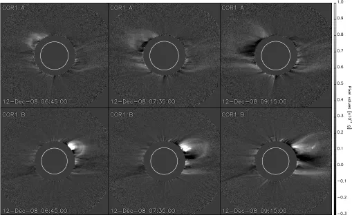
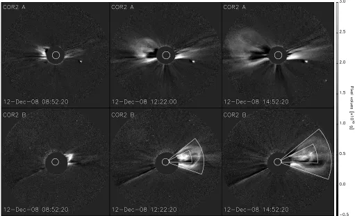
The COR1 images used in this analysis span from 2008 December 12 04:05 UT to 15:45 UT, with a ca-dence of 10 minutes. The three polarization states of COR1 were combined to make total brightness images in units of mean solar brightness (MSB). Base difference images were produced using the 04:05 UT image (in both COR1 A and B) as a background to be subtracted from all subsequent images. A sample of such images for both COR1 A and B can be found in Figure 1. The COR2 images analyzed range from from 07:22 UT to 17:52 UT, with a cadence of 30 minutes. As with the COR1 images, total brightness images were created for COR2, and a set of base difference images were then produced using the 07:22 UT image as a suitable background. A selected set of images from COR2 can be found in Figure 2.
At 04:35 UT the leading edge of a CME appeared in COR1 A and B coronagraphs at a height of∼1.4R, off the east and west limb respectively. In COR1 B the CME first appears as a set of rising loop-like structures followed by a prominence, part of which appears to fall back to the surface at 08:00 UT while the remainder was ejected and follows the rising loop-like structures which eventu-ally become the CME front. The rising prominence was not apparent at any stage of the propagation in COR1 A and the advancing front remains the only distinguishable facet of the CME from this line-of-sight (LOS).
A noteworthy caveat of using base difference imaging is the assumption that the background corona in the pre-event image has the same brightness in all subsequent images. This may not always be true and any excess brightness in the pre-event image will produce negative pixel values in the base difference. This is apparent in the COR1 images as the CME interacts with a streamer, dis-placing it as the leading CME front expands laterally as well as moves outward. The streamer is visible as a dark feature that grows with time at the southward flank of the CME in the COR1 B images, Figure 1. The black ar-eas are indicative of negative pixel values. The COR1 A images also suffer from negative pixels, especially at later
the three part structure of core, cavity, and bright front is clearly visible and the overall structure grows in size as the CME propagates to larger heights. The core be-comes more tenuous and the mass distribution bebe-comes homogenous after 15:52 UT when the front starts to exit the field of view. The distinction between core and front is not as clear in COR2 A and the mass distribution ap-pears more homogenous throughout the propagation. As with the COR1 images, COR2 A is also affected by ex-cess brightness in the pre-event image, as is apparent by a growing dark feature in its southern half. As the pre-event image for COR2 B is the cleanest of the pre-pre-event images (it contains the least contamination by stream-ers), the COR2 B data are considered the best candidate for accurate CME mass measurements.
3. CME MASS MEASUREMENT METHODS
The method by which mass measurements are derived from white light coronagraph images is based on theory first developed by Minnaert (1930) in which the scatter-ing geometry of a sscatter-ingle electron at a particular point in the solar atmosphere is considered. Further develop-ment of the theory by van de Hulst (1950) led to the derivation of what are now known as the van de Hulst coefficients. The coefficients treat each component of the incident electric field vector separately and take into ac-count the finite size of the solar disk (Minnaert 1930; Billings 1966; Howard & Tappin 2009). An important fact arising from these expressions is the dependence of scattering intensity on the angle, χ, between the radial vector from sun centre to the scattering electron and a position vector from observer towards the electron–the LOS, see Figure 3. Scattering efficiency is minimized when this angle is 90◦. However, along the LOS such an angle occurs at the point of minimum distance from sun centre where the incident intensity (that the elec-tron receives) and elecelec-tron density are maximized. This means scattered light in the corona is most intense along a plane perpendicular to the observer’s LOS despite the efficiency of scattering being minimized at such viewing angles (Howard & Tappin 2009). This plane perpendic-ular to the LOS is known as the plane-of-sky (POS)
Studies using single LOS coronagraph data are often hindered by the unknown CME propagation angle from the POS, e.g., unknown θ(orχ) in Figure 3. This leads to the incorrect angle being used when inverting the van de Hulst coefficients to calculate the number of electrons contributing to the scattered light. Furthermore, because the 3-D extent of the CME is unknown it is also assumed that the CME is confined to the 2-D sky plane, leading to a significant CME mass underestimation (Vourlidas et al. 2000).
Fig. 1.—Selection of base difference images of the CME in COR1 A (top row) and COR1 B (bottom row), with pixel values of grams. The CME is quite faint in the A images and appears not to have as much structure as in B. There is a large contribution to mass from a near-saturated region to the upper flank of the CME in the B images. Such saturation in the mass images coincides spatially with the prominence in total brightness images.
MSB to grams via the expression
mpixel=
Bobs
Be
×1.97×10⁻²⁴g (1)
where Bobs is the observed MSB of the pixel, Be is the electron brightness calculated from the van de Hulst co-efficients, and 1.97×10⁻²⁴g is a factor that converts the number of electrons to mass, assuming a completely ion-ized corona with a composition of 90% hydrogen and 10% helium. The known angle of propagation allowed the correct value ofBeto be computed resulting in a sig-nificant reduction in the uncertainties associated with the propagation angle. The largest remaining uncertainty is the unknown angular width along the LOS. This uncer-tainty was quantified in a similar approach to the method outlined in Vourlidas et al. (2000). This simulates the brightness of a CME with homogeneous density distribu-tion and finite angular width along the LOS–longitudinal angular width ∆θlong, allowing calculation of a simulated observed mass. Comparing this to the actual mass al-lowed for an evaluation of CME mass underestimation for given values of ∆θlong. Since the values for ∆θlongare unknown, the expression derived in Byrne et al. (2010) for thelatitudinal angular width of this CME as a func-tion of height, ∆θlat(r) = 25r0.22, was used to define an upper limit to ∆θlong. It was assumed the CME longitu-dinal angular width is no more than twice the latitudi-nal angular width, or ∆θlong62×∆θlat. Such an upper limit is in agreement with simulations of flux-rope CMEs
which give a typical aspect ratio of broadside to axial an-gular extents of 1.6 – 1.9 (Krall & St. Cyr 2006). Hence the value for ∆θlong at each height was used to obtain the simulated mass underestimation estimates described above. The heights and angular widths used in this study produced CME mass underestimation estimates of be-tween 5–10% for finite angular width uncertainty. An extra mass uncertainty of 6% was added to account for the assumption of coronal abundance of 90% hydrogen and 10% helium which can lead to slight errors while converting from pixel values of MSB to grams (Vourlidas et al. 2010).
Fig. 2.—Selection of base difference images of the CME in COR2 A (top row) and COR2 B (bottom row), with pixel values of grams. The CME is clearly distinguishable in both fields of view. Only the B field view shows clearly the three part structure of core, cavity and front. The COR2 B images were used to measure core and front mass separately
!
POS
L
O
S
P
Sun
χ
C∟
Fig. 3.—Schematic showing the relative orientation of the line-of-sight (LOS), and the plane-of-sky (POS). Electron position is at point P and C is Sun center. The vector CP may also repre-sent CME propagation direction. Scattering efficiency is heavily dependent on the angleθ(orχ) and is least efficient whenθ= 0◦ (χ= 90◦).
standard error on the mean. This standard error was de-fined as the uncertainty due to user bias in the point and click method of CME identification. The height at each measurement interval was taken to be the heliocentric distance of the CME apex in the image i.e., the apex of the front was chosen by simple point-and-click method. The uncertainty on the apex height was also found by the standard error on five runs.
The deflection of a small streamer during CME prop-agation produces negative pixels in the base difference images. The effect is particularly apparent in the COR1 images, Figure 1. It is difficult to unambiguously distin-guish between streamer and CME, making it difficult to quantify the uncertainty introduced due to streamer in-teraction. To make an estimate of the streamer’s effects, a calculation of its mass in the pre-event image was made. A number of different samples of the area of the streamer in the COR1 B pre-event image that effects all subse-quent images produced a mass estimate of ∼5×10¹⁴g. This mass was used as a measure of the uncertainty in-troduced due to streamer interaction in the COR1 B im-ages. A similar analysis of the COR1 A pre-event images gave a streamer mass estimate of ∼7×10¹⁴g. COR2 im-ages are relatively unaffected by significant changes in background coronal brightness and do not suffer from negative pixel values to as large an extent as COR1. The pre-event image of COR2 B is particularly clean and free of background streamers, hence COR2 B images are con-sidered to provide most accurate CME mass estimation. Finally, in order to obtain a more complete and con-tinuous estimate of CME mass growth, the masses deter-mined from both COR1 and COR2 coronagraphs were summed in those cases where image times of the inner and outer coronagraphs overlapped3. The overlap in the
3 A difference in cadence of the inner and outer coronagraphs
[image:4.612.64.277.431.587.2]inner and outer corongraphs’ fields of view was also taken into account in this summation.
A concise measurement of the CME kinematics, such as velocity and acceleration, were taken from the results of the study of Byrne et al. (2010). Since these kinemat-ics take into account the true three dimensional surface of the front they provide reliable estimates of CME ve-locity and acceleration in 3-D space. These veve-locity and acceleration measurements were used in the calculation of kinetic energy and total force on the CME for each point in time. The CME mass used in all energy and force calculations was the asymptotic mass it approaches at later stages of its evolution beyond 10Ras observed from theSTEREO Bspacecraft i.e., 3.4±1.0×10¹⁵g. As will be shown, there is good motivation for the use of con-stant mass in the magnitude of kinetic energy and force estimates.
4. RESULTS
4.1. CME Mass Estimates
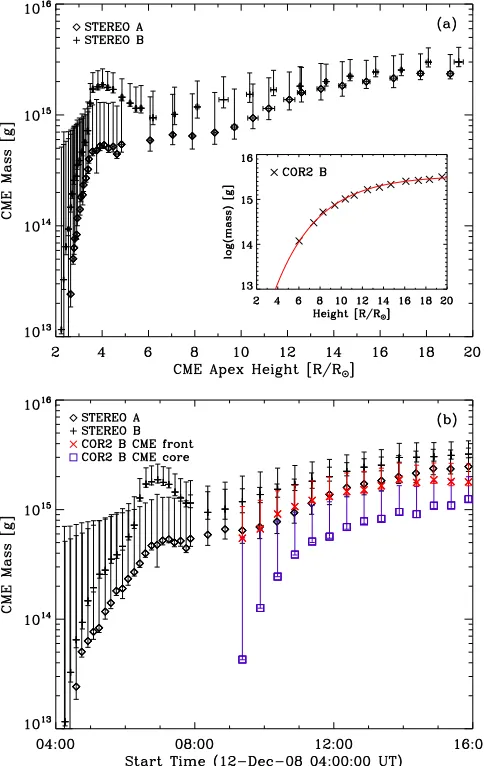
The results of the calculation for CME mass develop-ment with time and height for both STEREO A and B coronagraphs are shown in Figure 4. In panel (a), the height values are those taken from a point-and-click method of tracking the CME apex; these heights are cor-rected for CME propagation angle of∼45◦. In both pan-els (a) and (b), the mass estimates ofSTEREO A and B follow a similar trend and have similar values at each stage in the propagation. Such good agreement between mass values is a good indicator that ∼45◦ is the cor-rect angle of propagation from the sky-plane. A change in the cadence of mass measurements is noticeable at
[image:5.612.318.560.68.451.2]∼08:00 UT (or &5R). This is due to the use of only COR1 images (with a cadence of 10 minutes) prior to this time, and the use of the COR2 plus COR1 images af-ter this time (the cadence of these measurements follows that of COR2 – 30 minutes). Comparing A and B below 4.5R, mass values show a similar trend and increase at the same rate, but at approximately 3Rthe mass mea-surements in COR1 B appear to increase to a much larger value then fall again. This effect is visible in the COR1 A measurements, albeit diminished. It is probably due to the presence of a prominence which contains a significant mass content and therefore contributes a large amount to total measured CME mass. Also, early on in its prop-agation, the prominence may still be emitting H-αline radiation (656.28 nm) due to the larger fraction of neutral hydrogen at its cooler temperatures. The COR1 imag-ing passband is centered on H-α so any emission in the prominence from neutral hydrogen could be contributing to light received by the COR1 coronagraphs, this is ap-parent from the saturation region in the COR1 B images in Figure 1. Since this is resonance line emission, and not Thomson scattered emission, it leads to an erroneous measurement in CME mass. Thus, it is assumed the larger rise and fall in CME mass is caused by the promi-nence entering and exiting the COR1 B field of view. The effect is diminished in COR1 A since the prominence does not enter the FOV to as large an extent as in COR1 B. The interpretation that the ‘mass bump’ is not actual mass growth (or loss) is supported by previous measure-ments where CME mass increase follows a trend with height described by Mcme(h) =Ma(1−e−h/ha), where
Fig. 4.—CME mass development with height (a) and time (b), for the 2008 December 12 CME. After ∼08:00 UT (&5R) the
masses from the inner and outer coronagraphs are summed to show uninterrupted mass development from∼2–20Rover a
pe-riod of 12 hours. The small bump in the CME mass at∼07:00 UT (∼4R) is probably due to an unknown amount of H-αemission
from the prominence. Mass of CME front and core are also shown, red ‘×’ and blue square, for COR2 B, panel (b). After 14:52 UT they share approximately equal mass. The inset of (a) shows mass development with height for COR2 B only; the red curve repre-sents a fit to the data whereby the mass asymptotically approaches 3.4 ±1.0×10¹⁵g.
Mais the final mass the CME approaches asymptotically and ha is the height at which the CME reaches 0.63Ma (Colaninno & Vourlidas 2009), with no ‘bump’ in mass earlier on. The decline in mass after the peak may be ex-plained by the ionization of neutral hydrogen such that H-αemission diminishes and simply becomes Thomson scattering of free electrons, as with the rest of the CME material.
In order to produce a fit to the data, the COR2 B mass results were chosen because its pre-event image was largely free of any bright streamers or other features which introduce unwanted effects in the production of base difference images, as described above. A fit with the above equation resulted in a final asymptotic CME mass of 3.4±1.0×10¹⁵g, with a scale height ofh
in-dard error user-generated uncertainty, and uncertainty due to streamer interaction.
In each image where the CME core and front are distin-guishable, their masses were measured separately. This was carried out by user selected regions demarcating the areas of core and front, see COR2 B at 12:22 UT and 14:52 UT in Figure 2 for an example of the separate core and front sectors over which pixel values were summed to obtain total mass. The uncertainties due to finite width of the observed object also apply to the core and front measurements, however, since the widths of these partic-ular areas of the CME are unknown we chose the max-imum uncertainty of 10% from the above analysis since neither core nor front can be any wider than the max-imum width assigned to this CME. The remaining un-certainties described above were also applied. The mass development of core and front with time is shown in Fig-ure 4(b). The two mass measFig-urements are subject to an observational effect of apparent exponential mass growth, however by the time the CME is fully in the field of view at 14:45 UT the core and front share approximately equal mass.
4.2. CME Forces and Energetics
In the following calculations, all measurements of force and kinetic energy use the asymptotic mass of 3.4±1.0×10¹⁵g and not the instantaneous mass values calculated from each coronagraph image i.e., the CME is considered to begin its propagation with this mass and does not acquire any mass as it propagates.
Estimates of the force and kinetic energy use the 3-D velocity and acceleration measurements produced by Byrne et al. (2010). Their method firstly identifies the CME front in each coronagraph image using a multiscale edge detection filter. The front edges were then used to define a quadrilateral in space into which an ellipse is fit, this method is known as elliptical tie-pointing. This was done for multiple horizontal planes through the CME so that the fit ellipses outline a curved front in 3-D space. The speed and acceleration were then deduced from the change in position of the front, with time, through the
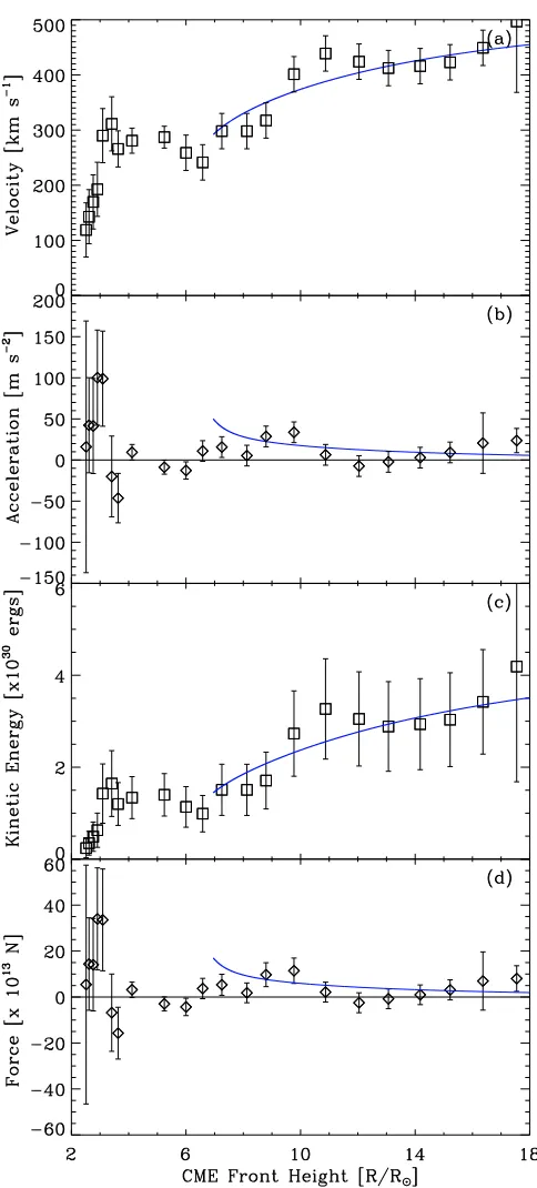
STEREO COR1, COR2 and HI fields of view. Since mass measurements in this study use only the COR1 and COR2 coronagraphs, HI kinematics measurements have been excluded here. The CME front position uncertainty inSTEREO AandBcoronagraphs was determined from the filter width in the multiscale analysis. Velocity and acceleration uncertainties were then propagated from po-sition uncertainty. Figure 5(a) shows CME velocity as a function of heliocentric distance, along with acceleration in panel (b).
[image:6.612.317.559.64.599.2]The CME kinetic energy was calculated usingEkin = 1/2Mcmev2cme, whereMcme is the final asymptotic mass of 3.4±1.0×10¹⁵g andvcmeare the instantaneous veloc-ity measurements, results of this calculation are shown in Figure 5(c). The kinetic energy shows an initial rise towards 6.3±3.7×1029ergs at ∼3R, beyond which it
Fig. 5.—(a) CME velocity as a function of heliocentric distance, including a fit to the data produced using an aerodynamic drag model beyond∼7R(Byrne et al. 2010). (b) Acceleration of CME,
including fit, derived from the velocity data and fit. Panel (c) and (d) show the kinetic energy and force, respectively, both calculated using constant CME mass of 3.4 ±1.0×10¹⁵g and kinematics
results from (a) and (b). Also shown are the fits to energy and force produced from fits to velocity and acceleration.
rises steadily to 4.2±2.5×1030ergs at∼18R, these val-ues are similar to those reported in Vourlidas et al. (2000, 2010) and Emslie et al. (2004).
The total force on the CME was calculated using
acme is taken from the instantaneous acceleration val-ues. As shown in panel (d) of Figure 5, the force ini-tially grows significantly, reaching a maximum value of 3.4±2.2×10¹⁴N at ∼3R
. The early rise and fall in acceleration (or force) is in agreement with a previous study of a CME observed to reach peak acceleration at
∼1.7R after which it reaches a constant velocity be-yond∼3.4R (Gallagher et al. 2003). Such results are also found in a statistical study which shows that the ma-jority of CMEs have peak acceleration in the low corona with a mean height of maximum acceleration at 1.5R (Bein et al. 2011). Similarly, observational studies by Zhang et al. (2001) and Zhang et al. (2004) also show early phase peak acceleration between 2–5Rand forces on the order of 1015N and 1012N, depending on whether the CME shows large initial acceleration or a slow, more gradual acceleration.
After this early peak, the force drops to an average value of 3.8±5.4×10¹³N at distances between 7–18R. It is apparent from Figure 5(a) that the velocity con-tinues to increase beyond 7R, implying that a positive radial force must be present. To clarify this, a fit to the velocity data using a model for solar wind drag on the CME beyond 7R (as outlined in Byrne et al. (2010)) is shown in Figure 5(a). Although the data suggest a non-monotonic increase in velocity, the fit reveals that propagation is best described by a steadily increasing velocity between 7–18R. The acceleration and kinetic energy curves derived from this velocity fit are shown in Figure 5(b) and (c). In Figure 5(d), the curve for the force derived from the velocity fit initially deviates from the data at ∼7R, however beyond this distance there is good agreement with the data and the derived force is entirely positive. This suggests that the solar wind exerts a positive aerodynamic drag force on the CME, resulting in a velocity that approaches the asymptotic solar wind speed at large heliospheric distances.
5. DISCUSSION
It should be noted that Figure 4 shows an overall expo-nential increase in CME mass with height which could be interpreted as the CME rapidly gaining mass as it prop-agates. Care should be taken with this interpretation since this apparent exponential mass increase is almost certainly due to the CME moving into the field of view, therefore allowing us to measure more of its mass con-tent; such an interpretation is in agreement with similar assertions made in Vourlidas et al. (2010). It is difficult to distinguish between actual CME mass growth and an ap-parent growth due to more of the CME being observed. If the initial early rise in CME mass is assumed to be an observational artifact then we can interpret the CME mass to be in the range of (3–3.5)×1015g for most of its early propagation i.e., the CME already has such a mass before launch and does not acquire more mass (via inflows or otherwise) during propagation. Such an inter-pretation is in agreement with CME mass measurements calculated from dimmings in STEREO Extreme Ultra-violet Image (EUVI) images, which show the mass cal-culated from EUV images to be approximately equal to CME mass in COR2 images,mEU V I/mCOR2= 1.1±0.3 (Aschwanden et al. 2009). Once the CME bubble is in the field of view at∼10R the mass in its entirety can be measured and the increase beyond this point, if any,
is slow and steady, Figure 4.
The early stages of CME propagation are dominated by a sharp rise to a peak force of 3.4±2.2×10¹⁴N at∼3R
followed by a sharp decline, Figure 5(d). The catastrophe model (Forbes & Isenberg 1991; Forbes & Priest 1995; Lin & Forbes 2000), magnetic breakout model (Antio-chos et al. 1999; Lynch et al. 2008), and toroidal insta-bility model (Chen 1996; Kliem & T¨or¨ok 2006) employ a number of forces acting on the CME to produce an over all acceleration into interplanetary space. For example, the toroidal instability model used by Chen (1996) uses a Lorentz hoop force (or Lorentz self-force), solar wind drag, and gravity to provide a net force acting on the CME between 2–3R that quickly rises to a peak total force of ∼1016N and then falls rapidly.
If we assume that the peak force observed for the 2008 December 12 CME is the net force due to similar forces used in the above models, such as the solar wind drag, gravity, and some form of magnetic CME driver e.g., a
~
J ×B~ force, we may estimate their relative contribution. The force due to solar wind drag on the CME is given by
~ Fd =−
1
2CdρswAcme(~v−v~sw)| ~v−~vsw| (2) where Mcme is the CME mass, ~v is the CME velocity,
Cd is the drag coefficient, ρsw is the solar wind mass density, Acme is the CME area exposed to solar wind drag and~vsw is the solar wind velocity (Maloney & Gal-lagher 2010). To estimate the effects of this force we use
ρsw =npmp, where mp is proton mass, and assume ion-ization fraction of χ= 1 such thatnp=ne[cm−3]. Elec-tron density, and hence proton density, is then given by an interplanetary density model derived from a special solution of the Parker solar wind equation (Mann et al. 1999), solar wind velocity values as a function of height are also determined using this model. Acmeis estimated using the expression derived in Byrne et al. (2010) for latitudinal angular width of the CME as a function of height, ∆θlat(r) = 26r0.22. This is used to derive an arc length of the CME front and, as above, making the as-sumption ∆θlong= 2×∆θlat, the two arc lengths derived from these angles then give the surface that the solar wind acts on, thus Acme= 1352r2.44. Setting the drag coefficient Cd = 1, and using the Mann et al. (1999) model to derive a density and a solar wind velocity of 2.3×105cm−3 and 70 km s−1, respectively, equation [1] then gives a force ofF~d=−8.0×10¹²rˆN for solar wind drag at ∼3R, where ˆr is a unit vector in the positive radial direction.
A simple estimate of force due to gravity is given by
~
Fg =GMMcme/~r2, where Gis the universal gravita-tional constant, M is solar mass, Mcme is CME mass, and ~r is a heliocentric position vector4. Given a CME mass of 3.4×10¹⁵g the force due to gravity at a heliocen-tric distance of 3R is F~g =−1.0×10¹⁴rˆN. The only remaining contribution is due to some form of magnetic
4 Ideally the heliocentric distance of the CME centre of mass
Using the above values, the total magnetic contribution to CME force is calculated to beF~mag≈4.5×10¹⁴ˆrN at 3R, indicating that this is the largest driver of CMEs at low coronal heights. Lorentz force dominated dynam-ics in early phase CME propagation are reported in Bein et al. (2011), in which a statistical study of a large sam-ple of CMEs in EUVI, COR1, and COR2 indicated an early phase acceleration for the majority of CMEs that is attributable to a Lorentz force. A similar result of an observational study by Vrˇsnak (2006) found that the Lorentz force plays a dominant role within a few solar radii. It should be noted that although we have labelled the forceFmag, there is no distinction on the exact form of this force e.g., whether it is magnetic pressure, mag-netic tension, or a Lorentz self-force that acts as the driver. Also, any non-radial motion of the CME, such as that described in Byrne et al. (2010), is not taken into account here; any force estimates are purely radial in direction.
6. CONCLUSION
TheSTEREO COR1/2 coronagraphs have been used to determine the mass development of the 2008 Decem-ber 12 CME. Knowledge of the longitudinal propaga-tion angle of the CME allowed for a significant reduc-tion in the mass uncertainty, giving a final estimate of 3.4±1.0×10¹⁵g. Using kinematics results of a previous study (Byrne et al. 2010), the velocity and acceleration of the CME were combined with the mass measurements
celeration) is in agreement with previous observations of CME kinematics (Gallagher et al. 2003; Bein et al. 2011). Similarly results of observational studies by Zhang et al. (2001) and Zhang et al. (2004) also show early phase peak acceleration between 2–5R and forces on the or-der of 1015N and 1012 N. The kinetic energy shows an initial rise towards 6.3±3.7×1029ergs at∼3R
, beyond which it rises steadily to 4.2±2.5×1030ergs at∼18R, such order of magnitudes are similar to those reported in Vourlidas et al. (2000); Emslie et al. (2004) and are typical of CME kinetic energies (Vourlidas et al. 2010).
Such CME kinematics and dynamics property esti-mates cannot be carried out when unknown propaga-tion angle hinders an accurate calculapropaga-tion of CME mass, hence adding unacceptable uncertainty to any subse-quent calculations. This highlights the need for similar studies using theSTEREOmission’s ability to accurately determine the physical properties of CMEs, such as mass, with remarkably reduced uncertainty. Increasing the ac-curacy of force estimates of other well studied CMEs will allow for a more complete view of the magnitude of the forces influencing CME propagation and will allow model parameters to be more accurately constrained.
This work is supported by the Irish Research Coun-cil for Science, Engineering and Technology (IRC-SET). We also extend thanks and appreciation to the
STEREO/SECCHI consortium for providing open access to their data.
REFERENCES
Antiochos, S. K., DeVore, C. R., & Klimchuk, J. A. 1999, ApJ, 510, 485
Aschwanden, M. J., Nitta, N. V., Wuelser, J.-P., Lemen, J. R., Sandman, A., Vourlidas, A., & Colaninno, R. C. 2009, ApJ, 706, 376
Bein, B. M., Berkebile-Stoiser, S., Veronig, A. M., Temmer, M., Muhr, N., Kienreich, I., Utz, D., & Vrˇsnak, B. 2011, ApJ, 738, 191
Billings, D. E. 1966, A guide to the solar corona, ed. Billings, D. E.
Brueckner, G. E., et al. 1995, Sol. Phys., 162, 357
Byrne, J. P., Maloney, S. A., McAteer, R. T. J., Refojo, J. M., & Gallagher, P. T. 2010, Nature Communications, 1
Chen, J. 1996, J. Geophys. Res., 1012, 27499
Chen, J., Marqu´e, C., Vourlidas, A., Krall, J., & Schuck, P. W. 2006, ApJ, 649, 452
Colaninno, R. C., & Vourlidas, A. 2009, ApJ, 698, 852
Domingo, V., Fleck, B., & Poland, A. I. 1995, Sol. Phys., 162, 1 Emslie, A. G., et al. 2004, Journal of Geophysical Research
(Space Physics), 109, A10104
Forbes, T. G., & Isenberg, P. A. 1991, ApJ, 373, 294 Forbes, T. G., & Priest, E. R. 1995, ApJ, 446, 377
Gallagher, P. T., Lawrence, G. R., & Dennis, B. R. 2003, ApJ, 588, L53
Howard, R. A., et al. 2008, Space Sci. Rev., 136, 67
Howard, T. A., Fry, C. D., Johnston, J. C., & Webb, D. F. 2007, ApJ, 667, 610
Howard, T. A., & Tappin, S. J. 2009, Space Sci. Rev., 147, 31 Kaiser, M. L., Kucera, T. A., Davila, J. M., St. Cyr, O. C.,
Guhathakurta, M., & Christian, E. 2008, Space Sci. Rev., 136, 5 Kliem, B., & T¨or¨ok, T. 2006, Physical Review Letters, 96, 255002
Krall, J., & St. Cyr, O. C. 2006, ApJ, 652, 1740
Lin, C.-H., Gallagher, P. T., & Raftery, C. L. 2010, A&A, 516, A44
Lin, J., & Forbes, T. G. 2000, J. Geophys. Res., 105, 2375 Lynch, B. J., Antiochos, S. K., DeVore, C. R., Luhmann, J. G., &
Zurbuchen, T. H. 2008, ApJ, 683, 1192
Maloney, S. A., & Gallagher, P. T. 2010, ApJ, 724, L127 Mann, G., Jansen, F., MacDowall, R. J., Kaiser, M. L., & Stone,
R. G. 1999, A&A, 348, 614
Manoharan, P. K., & Kundu, M. R. 2003, ApJ, 592, 597 Minnaert, M. 1930, ZAp, 1, 209
Munro, R. H., Gosling, J. T., Hildner, E., MacQueen, R. M., Poland, A. I., & Ross, C. L. 1979, Sol. Phys., 61, 201 Poland, A. I., Howard, R. A., Koomen, M. J., Michels, D. J., &
Sheeley, Jr., N. R. 1981, Sol. Phys., 69, 169
Schrijver, C. J., Elmore, C., Kliem, B., T¨or¨ok, T., & Title, A. M. 2008, ApJ, 674, 586
van de Hulst, H. C. 1950, Bull. Astron. Inst. Netherlands, 11, 135 Vourlidas, A., Buzasi, D., Howard, R. A., & Esfandiari, E. 2002,
in ESA Special Publication, Vol. 506, Solar Variability: From Core to Outer Frontiers, ed. A. Wilson, 91–94
Vourlidas, A., Howard, R. A., Esfandiari, E., Patsourakos, S., Yashiro, S., & Michalek, G. 2010, ApJ, 722, 1522
Vourlidas, A., Subramanian, P., Dere, K. P., & Howard, R. A. 2000, ApJ, 534, 456
Vrˇsnak, B. 2006, Advances in Space Research, 38, 431
Zhang, J., Dere, K. P., Howard, R. A., Kundu, M. R., & White, S. M. 2001, ApJ, 559, 452