http://www.sciencepublishinggroup.com/j/ijiis doi: 10.11648/j.ijiis.20190804.12
ISSN: 2328-7675 (Print); ISSN: 2328-7683 (Online)
Constrained Blind Separation Algorithm Using Variable
Step Size and Variable Momentum Factor
Liu Lu, Ou Shifeng
*, Gao Ying
School of Science and Technology for Opto-electronic Information, Yantai University, Yantai, China
Email address:
*
Corresponding author
To cite this article:
Liu Lu, Ou Shifeng, Gao Ying. Constrained Blind Separation Algorithm Using Variable Step Size and Variable Momentum Factor. International Journal of Intelligent Information Systems. Vol. 8, No. 4, 2019, pp. 77-84. doi: 10.11648/j.ijiis.20190804.12 Received: October 15, 2019; Accepted: November 14, 2019; Published: November 18, 2019
Abstract:
The traditional blind separation algorithm is mainly for the instantaneous mixing problem in the stable environment. In the practical applications, blind separation often takes into account the interference of the external environment, which requires that the algorithm has strong tracking performance, but the traditional algorithm can’t meet the needs. Aiming at the problem of instantaneous blind separation in non-stationary environment, constrained blind separation algorithm using variable step size and variable momentum factor is proposed in this paper. Based on the nonholonomic natural gradient algorithm, the cost function is constrained by the disturbance of the hybrid system and the constraint factors take the form of self-adaptive adjustment. According to the separation situation, the constraint factors are adjusted adaptively to accelerate the convergence speed. The variable step size based on the cost function gradient is introduced to improve the tracking performance. By incorporating momentum term, the momentum factor is adaptively adjusted to make it have better separation performance. The simulation results show that compared with the traditional algorithm, the proposed algorithm can better balance the contradiction between convergence speed and steady-state error in non-stationary environment, and has better separation performance. In the case of obvious disturbance in the mixed system, the algorithm can effectively improve the shortcomings of the traditional algorithm. In summary, constrained blind separation algorithm using variable step size and variable momentum factor proposed in this paper is effective.Keywords:
Blind Separation, Non-stationary, Nonholonomic Natural Gradient, Adaptive, Momentum Factor1. Introduction
Blind source separation (BSS) refers to the recovery of source signals from a set of observed signals only according to the statistical independence of each source signal when the source signal and the mixed system are unknown. The “blind” means that the source signal cannot be directly observed and the hybrid system is unknown. In recent years, blind separation technology has made continuous progress and has been widely used in biomedical signal processing, wireless communication, speech recognition, feature extraction and data compression [1, 2]. Blind separation has uncertainty, which is reflected in the difference in magnitude and order of the source signals recovered by the separation matrix. In fact, it is multiplying the arbitrary row vector of the separation matrix by a fixed scale factor or exchanging the position of any row vector, but it will not affect blind separation in
essence. In the non-stationary environment, blind separation can be divided into three conditions: 1) the source signal is non-stationary when the mixed system is invariable; 2) the source signal is stationary when the mixed system is time-varying; 3) the source signal is non-stationary when the mixed system is time-varying. This paper mainly studies the second conditions, that is, the mixed system is time-varying. At this time, the external environment is non-stationary due to the existence of system disturbance.
crosstalk error, and proposed a new variable step-size method based on blind source separation reference separation system. Reference [5] increases the variable step size of the cost function gradient, and proposed the nonholonomic natural gradient algorithm based on sign operator. Reference [6] aiming at the difficulty in selecting nonlinear functions, and proposed an algorithm for selecting the appropriate activation function adaptively by kurtosis. Reference [7] established a new separation measurement index, constructed a nonlinear monotone function, adaptive adjustment of the step size and momentum factor, and proposed an adaptive blind separation method of variable step size momentum term. Reference [8] based on the separation performance index, the approximate optimal parameters are designed, and proposed the step-size adaptive blind source separation algorithm with adding momentum term. Reference [9, 10], a variable step size blind source separation algorithm with adaptive momentum factor was proposed by using the construction function of the performance evaluation index of the separation signal. Reference [11] proposed an adaptive variable step size algorithm in non-stationary environment by using the disturbance of mixed system, constraint cost function, adaptive constraint factor and step size.
The above literature uses different methods to improve the algorithm, which has a good separation effect to some extent, but the contradiction between convergence speed and steady-state error hasn't been well improved. Aiming at the shortcomings of the above algorithms, constrained blind separation algorithm using variable step size and momentum factor is proposed, which is suitable for non-stationary environments. Firstly, based on the nonholonomic natural gradient algorithm, introduce gate function and constraint cost function. According to the separation situation, the constraint factors are adjusted adaptively. Secondly the variable step size based on the cost function gradient is introduced to improve the tracking performance. Thirdly the momentum term is integrated, and the momentum factor takes an adaptive form, thereby accelerating the convergence speed and reducing the steady-state error. In the case of obvious disturbance in the mixed system, the algorithm can effectively improve the shortcomings of the traditional algorithm. Finally, the simulation results show that the algorithm is effective.
2. Constrained Nonholonomic Natural
Gradient Algorithms in
Non-stationary Environment
2.1. Blind Source Separation and Nonholonomic Natural Gradient Algorithm
Without considering the noise interference, the instantaneous mixing model of blind separation can be presented as:
x( )k =As( )k (1)
where Α represents the N×N row-full-rank mixed matrix,
1 2
x( )k =[ ( ),x k x k( ),⋯,xN( )]k Tis the N-dimensional mixed signal vector, s( )k =[ ( ),s k s k1 2( ),⋯,sN( )]k T is the N-dimensional source signal vector.
After separating the separation matrix, the estimated source signal is:
y( )k =Wx( )k =WAs( )k =Gs( )k (2)
where y( ) [ 1( ), 2( ), , ( )]
T N
k = y k y k ⋯ y k is the estimation
signal vector of the N-dimensional source signal, W is the separation matrix, and G is the N-dimensional global matrix.
The natural gradient algorithm [12] can find the optimal separation matrix Wept by successively correcting W ,
namely:
W(k+ =1) W( )k +
µ
( ) Ik −f(y( ))y ( ) W( )k T k k (3)where µ( )k is the step size, its affects the convergence speed and stability of the algorithm. When the value is large, the convergence speed is fast, but the stability is poor; when the value is small, the convergence speed is slow, but the stability is good. fi(y )i represents a non-linear activation function,define:
( ) ( )
( )
i i i i
i i
P y f y
P y
′
= − (4)
where Pi( )⋅ is the probability density function of the ith signal source. In general, when the signal source is a sub-Gaussian signal, the activation function chooses cubic function f y( )= y3 ; When the signal source is a super-Gaussian signal, the activation function chooses the hyperbolic tangent function f y( )=ay+tan( )ry .
Based on the natural gradient algorithm, Amari introduces an nonholonomic basis dX=dWW−1 to limit the possible change direction of δW , and the iterative formula of nonholonomic natural gradient (NNG) algorithm [13, 14] is obtained by combining equation (3), namely:
W(k+ =1) W( )k +µ( )[Λk − f(y( ))y ( )]W( )k T k k (5)
where Λ=diag
{
λ λ1, 2,⋯,λn}
represents the positivediagonal matrix of the elementλi = f(y )yi iT.
2.2. Constraint Algorithm in Non-stationary Environment
[15]. When the condition that g(W)≥0 and J(W) reach the minimum value is satisfied, Solving optimization problems, that is, Solving the minimum of the augmented cost function. The augmented cost function is:
A(W) (W) (W)
J =J +RB (6)
Where
{
}
1
(W) log det(W) log ( )
n
i i i
J E q y
=
=− −
∑
is the costfunction based on mutual information minimization. (W) ln (W)
B = − g is the logarithmic gate function, used to prevent feasible solutions from leaving the region determined by inequality constraints. R(W) is the constraint factor, used to control the gate function. The setting of constraint conditions is obtained by assuming the initial separation matrix and the disturbance added to the mixed matrix. Assuming A0 is the mixed system in the stationary environment (the mixed matrix without disturbance), D is the disturbance on the mixed system. Define the disturbance coefficient r= A0DF, according to the definition of matrix
norm: 1 0 1 0 A (A ) 1 F F D r − − + ≤
− (7)
Since A0+D stands for real-time mixed matrix,
1 0 (A +D)− can be replaced by W , which is the corresponding separation matrix. Similarly, A0−1 is replaced by W0, which is the initial separation matrix. Formula (7) can be written as follows:
0 W W
1
F
F ≤ −r (8)
Squared on both sides:
(
)
2 2 0 2 W W 1 F F r ≤− (9)
Inequality constraint is expressed as:
(
)
2 2 0 2 W (W) W 1 F F g r = −− (10)
From this, the logarithmic gate function can be obtained:
(
)
2 2 0 2 W(W) ln W
1 F F B r = − − − (11)
The augmented cost function can be expressed as
(
)
2 2 0 A 2 W(W) (W) ln W
1
F
F
J J R
r = − − − (12)
Can be obtained:
A(W) W( ) P( )W( ) M( )
J k k k R k
∂ ∂ = − − (13)
P( )k =[Λ− f(y( ))y ( )]k T k (14)
(
)
2
2 0
2 2W( )
M( ) [ ]
W W( ) 1 F F k k k r = − − (15)
Therefore, the iteration formula of the nonholonomic natural gradient algorithm (C-NNG) based on the constrained cost function is as follows:
W(k+ =1) W( )k +µP( )W( )k k +µRM( )k (16)
3. Adaptive Algorithm
3.1. Adaptive Constraint Factor
The selection of the constraint factor will have a certain impact on the algorithm. When the value of constraint factor is large, the convergence is fast but the stability is poor. In order to improve the shortcomings of the algorithm when the constraint factor is constant value, the constant value constraint factor in the algorithm is adjusted to the adaptive constraint factor, and the updated iteration equation of the adaptive constraint factor can be written as:
A ( 1)
( ) ( 1) R ( )R R k
R k =R k− − ∇ρ J k = − (17)
where ρ is a small constant.
According to the matrix inner product operation, the gradient term ∇RJA( )k R R k= ( −1) can be expressed as:
(
)
A ( 1)
A
A ( )
( ) W( ), W( ) ( 1)
( ) W( ) W( ) ( 1)
R R R k
T
J k
J k k k R k
tr J k k k R k
= −
∇
= ∂ ∂ ∂ ∂ −
= ∂ ∂ ×∂ ∂ −
(18)
where ∂W( )k ∂R k( − =1) µM(k−1) , ⋅ is the inner product, tr()is the trace of the matrix.
Equation (17) can also be represents as:
( ) ( 1) [( P( )W( )
( )M( )) ( M(T 1))]
R k R k tr k k
R k k k
ρ
µ
= − − −
− − (19)
Therefore, the iterative equation of the nonholonomic natural gradient algorithm (AC-NNG) based on the adaptive constraint factor is as follows:
3.2. Adaptive Variable Step Size
The step size has a great influence on the convergence speed and stability of the algorithm,fixed step size limits algorithm performance. When the step size is large, the convergence is fast but the stability is poor. When the value is small, the stability is good but the convergence is slow. In order to improve the shortcomings of the algorithm when the step size is fixed, the fixed step size is adjusted to adaptive variable step size, and the updated iteration formula of adaptive variable step size is as follows:
A ( 1)
( ) ( 1) ( )
k
k k µJ k
µ µ
µ =µ − − ∇λ = − (21)
where λ is a small constant.
According to the matrix inner product operation, the gradient term ∇µJA( )k µ µ= (k−1) can be expressed as:
(
)
A ( 1)
A
A ( )
( ) W( ), W( ) ( 1)
( ) W( ) W( ) ( 1)
k
T
J k
J k k k k
tr J k k k k
µ µ µ
µ µ
− −
∇
= ∂ ∂ ∂ ∂ −
= ∂ ∂ × ∂ ∂ −
(22)
where ∂W( )k ∂
µ
(k− =1) P(k−1)W(k− +1) R k( −1)M(k−1) Formula (21) can also be represents as:( ) ( 1) [( P( )W( ) ( )M( ))
(P( 1)W( 1) ( 1)M( 1))]
T
k k tr k k R k k
k k R k k
µ =µ − −λ − −
× − − + − − (23)
Therefore, the iteration formula of variable step size nonholonomic natural gradient algorithm (ACV-NNG) based on the adaptive constraint factor is as follows:
W(k+ =1) W( )k +µ( )P( )W( )k k k +µ( ) ( )M( )k R k k (24)
3.3. Adaptive Momentum Factor
Compared with the AC-NNG algorithm, the convergence speed of the ACV-NNG algorithm is improved, but the steady-state error is not significantly improved. Aiming at this phenomenon, in order to further improve the convergence speed and reduce the steady-state error, this paper incorporated the momentum term, when the momentum term is incorporated and the momentum factor is a constant value, the iterative formula of the algorithm (ACVM-NNG-fixed) is:
W( 1) W( ) ( )P( )W( )
( ) ( )M( ) [W( ) W( 1)]
k k k k k
k R k k k k
µ
µ β
+ = +
+ + − − (25)
where β[W( )k −W(k−1)] is the momentum term, and
β
represents the momentum factor.The above algorithm improves the convergence speed, but the steady-state error has not been significantly improved. In order to further improve the convergence speed and reduce the steady-state error, and better balance the contradiction between the convergence speed and the steady-state error. In
this paper, an adaptive form of the momentum factor is adopted, the update iteration formula of the adaptive momentum factor is:
A ( 1)
( )k (k 1) βJ ( )k β β k
β
=β
− − ∇σ
= − (26)where
σ
is a small constant.According to the matrix inner product operation, the gradient term ∇βJA( )k β β= (k−1) can be expressed as:
A ( 1)
A
A ( )
( ) W( ) , W( ) ( 1)
( ( ) W( ) W( ) ( 1))
k
T
J k
J k k k k
tr J k k k k
β β β
β β
= −
∇
= ∂ ∂ ∂ ∂ −
= ∂ ∂ ×∂ ∂ −
(27)
where ∂W( )k ∂β(k− =1) W(k− −1) W(k−2). Formula (24) can also be written as:
( ) ( 1) [( P( )W( ) ( )M( ))
(W( 1) W( 2))]
T
k k tr k k R k k
k k
β =β − −σ − −
× − − − (28)
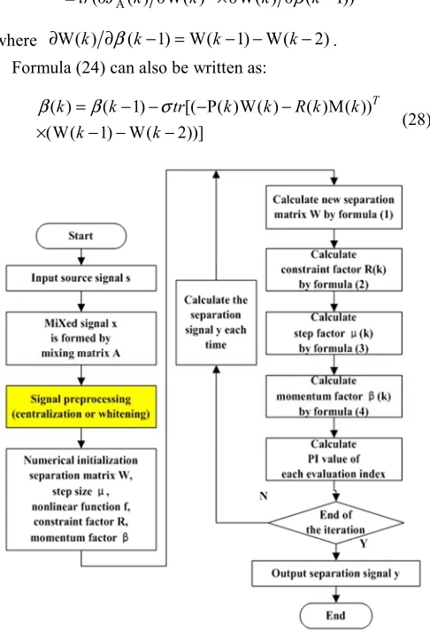
Figure 1. Algorithm flow.
Therefore, the iteration formula of variable step size momentum factor nonholonomic natural gradient algorithm based on adaptive constraint factor (ACVM-NNG) is as follows:
W( 1) W( ) ( )P( )W( )
( ) ( )M( ) ( )[W( ) W( 1)]
k k k k k
k R k k k k k
µ
µ β
+ = +
+ + − − (29)
can be adaptively adjusted according to the needs, which accelerates the convergence speed of the algorithm, reduces the steady-state error, and has better separation performance. The flow chart of the ACVM-NNG algorithm is shown in Figure 1.
4. Simulation Experiment
In order to verify the effectiveness of the proposed algorithm, simulation experiments are carried out under the non-stationary environment. The communication signals selected in this simulation experiment are: high frequency
sinusoidal signal s1=sin 2 800
(
π t)
, low frequency sinusoidal signal s2 =sin 2 90(
π t)
, sampling frequency10
f = kHz, disturbance coefficient r=0.2 and non-linear function f y( )=y3. Set NNG algorithm, C-NNG algorithm and AC-NNG algorithm step size
µ
=0.006, ACV-NNG algorithm, ACVM-NNG-fixed algorithm, ACVM-NNG algorithm initial step size µ =0 0.001 . To compare the separation performance of these six algorithms, select PI[16] as the performance evaluation index:
1 1 1 1
1 1
( ) 1 1
max max
= = = =
= − + −
∑∑
n m ij∑∑
n m ijj ij i ij
i j i j
g g
PI G
n g m g (30)
the smaller the value, the better the separation effect, and vice versa.
In the first case: at each sampling point, disturbances occur in the mixed system.
Set the time-varying mixed matrix:
0 0 0
A =A +0.001(randn size( (A ))) (31)
0
1.0 0.6 A
0.5 0.5
=
− −
(32)
0 ( (A ))
randn size means to generate a random matrix with the same dimension as A0 and each element between [0, 1], the momentum factor in ACVM-NNG-fixed algorithm
1 0.65
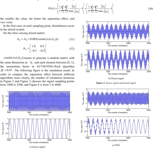
β = . The following figure is the simulation result. In order to compare the separation effect between different algorithms more clearly, the number of simulation iterations in Figure 2 and Figure 3 chooses the signal sampling points from 1000 to 2500, and Figure 4 is from 1 to 6000.
a) Source signal
b) Mixed signal
Figure 2. Source signal and mixed signal.
b) C-NNG
c) AC-NNG
d) ACV-NNG
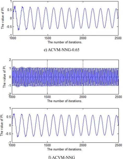
e) ACVM-NNG-0.65
f) ACVM-NNG
Figure 3. Source signals estimated by six algorithms.
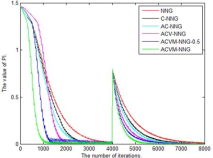
Figure 4. Separation performance curve.
It can be seen from Figure 3 that the source signals estimated by the newly proposed ACVM-NNG-Fixed algorithm and the ACVM-NNG algorithm can reach the convergence state with fewer iterations, the ACVM-NNG algorithm has faster convergence speed. It can be seen more clearly from figure 4 that, compared with the first four algorithms, the two newly proposed algorithms have faster convergence speed and less steady-state error, which can better balance the contradiction between the convergence speed and steady-state error. The ACVM-NNG algorithm has better effect.
In the second case: When the number of sampling points is 4000, there is a sudden change in the hybrid system.
0
1.0 0.6 A
0.5 0.5
=
− −
(33)
After the mutation occurs, set the mixed matrix:
1 1
A=A +0.01(rand size( (A ))) (34)
1
1.19 0.6 A
0.5 0.1
=−
(35)
the momentum factor in ACVM-NNG-fixed algorithm 2 0.5
β = . Figure 5 is the simulation result of the separation performance curve of the six algorithms, and the number of iterations is from 1-8000.
Figure 5. Separation performance curve.
As can be seen from Figure 5, in the case of mutation, the convergence speed of the two newly algorithms is faster than that the first four algorithms. The ACVM-NNG algorithm has faster convergence speed than the ACVM-NNG-Fixed algorithm, and the steady-state error is smaller, which can better balance the contradiction between convergence speed and steady-state error. In the case of mutation, the separation effect is better than that of the first case before the number of iterations is 4000, because there is no system disturbance before the mutations occurs, while in the first case, there are system disturbances at every sampling point. Comparing Figure 4 and Figure 5, the newly proposed ACVM-NNG algorithm has better effects in the presence or absence of mutation, It improves the convergence speed while reducing the steady-state error and has better separation performance. It can be seen that the variable step size momentum factor nonholonomic natural gradient algorithm based on adaptive constraint factor proposed in this paper is effective.
5. Conclusion
This paper mainly studies the mixed system with time-varying and stable source signals. On the basis of the nonholonomic natural gradient algorithm, considering the system disturbance, a new improved algorithm is proposed. The algorithm adopts a method of adaptively constraining
factor, step size and momentum factor to balance the relationship between convergence speed and steady state error. The simulation results show that the algorithm has better separation effect, and can improve the convergence speed and reduce the steady-state error.
Acknowledgements
This work is supported by the Natural Science Foundation of Shandong Province (No. ZR2017MF008).
References
[1] A. Cichocki, S. Amari, Adaptive Blind Signal and Image Processing: Learing Algorithms and Application. New York: Wiley Press, 2002, pp. 24-42.
[2] S. Y. Peng, Z. H. Wang, Y. Q. Zhu, “Present Situation and Development of Blind Source Separation,” Shipboard Electronic Countermeasure, vol. 39. 2016, pp. 54-57.
[3] W. C. Ding, H. Zhang, “Natural Gradient Blind Separation Algorithm for Optimal Search Direction,” Journal of Military communications Technology, vol. 38. 2017, pp. 12-16. [4] P. C. Xu, Y. H. Shen, Q. Su, “Blind source separation with
variable step-size method based on a reference separation system,” IEEE International Conference on Sinal Processing, Communications and Computing, 2014, pp. 110-114.
[5] C. Ji, K. Yang, Y. R. Wang, M. D. Liu, “Variable Step Size Nonholonomic Natural Gradient Algorithm Based on Sign Operator,” Pattern Recognition and Artificial Intelligence, vol. 27. 2014, pp. 1026-1031.
[6] Y. L. Niu, Y. M. Wang, Y. Wang, “Improved Adaptive Algorithm of Blind Source Separation Based on Nonholonomic Natural Gradient,” Pattern Recognition and Artificial Intelligence, vol. 19. 2006, pp. 667-673.
[7] Z. Y. Ma, T. Q. Zhang, Q. Li, X. M. Liang, “Adaptive Variable-step Blind Source Separation with Momentum Factor,” Telecommunication Engineering, vol. 59. 2019, pp. 294-300. [8] C. T. Li, Y. Z. Jiang, F. J. Liu, S. X. Zhang, “Step-size adaptive
blind source separation algorithm with adding momentum term,” Journal of Naval University of Engineering, vol. 31. 2019, pp. 107-112.
[9] T. Q. Zhang, B. Z. Ma, X. Z. Qiang, S. R. Quan, “Variable-step blind source separation method with adaptive momentum factor,” Journal on Communications, vol. 38. 2017, pp. 16-24.
[10] T. Q. Zhang, B. Z. Ma, X. Z. Qiang, S. R. Quan, “Variable-step Blind Source Separation Algorithm with Adaptive Momentum Item for Chaotic Signals,” Journal of Electronics and Information Technology, vol. 39. 2017, pp. 908-914.
[11] C. Ji, K. Yang, Y. M. Tao, X. Wang, “An adaptive variable step-size blind source separation algorithm in non-stationary environment,” Contyol and Decision, vol. 31. 2016, pp. 735-739.
[13] C. Ji, B. C. Tang, K. Yang, M. Sha, “Improved blind source separation based on nonholonomic natural gradient algorithm with variable step size,” 2013 China intelligent automation academic conference, 2013, pp. 761-767.
[14] S. Amari, T. P. Chen, A. Cichocki, “Non-Holonomic Constraints in Learning Algorithms for Blind Source Separation,” Neural Computation, vol. 12. 2000, pp. 1463-1484.
[15] Y. S. Xia, G. Feng, J. Wang, “A novel recurrent neural network for solving nonlinear optimization problems with inequality constraints,” IEEE Trans on Neural Networks, vol. 19. 2008, pp. 1340-1353.