https://doi.org/10.5194/amt-11-6589-2018 © Author(s) 2018. This work is distributed under the Creative Commons Attribution 3.0 License.
Joint retrieval of surface reflectance and aerosol properties with
continuous variation of the state variables in the solution space –
Part 1: theoretical concept
Yves Govaerts and Marta Luffarelli Rayference, 1030 Brussels, Belgium
Correspondence:Yves Govaerts ([email protected]) Received: 29 January 2017 – Discussion started: 7 March 2017
Revised: 26 November 2018 – Accepted: 30 November 2018 – Published: 14 December 2018
Abstract.This paper presents a new algorithm for the joint retrieval of surface reflectance and aerosol properties with continuous variations of the state variables in the solution space. This algorithm, named CISAR (Combined Inversion of Surface and AeRosol), relies on a simple atmospheric ver-tical structure composed of two layers and an underlying sur-face. Surface anisotropic reflectance effects are taken into ac-count and radiatively coupled with atmospheric scattering. For this purpose, a fast radiative transfer model has been ex-plicitly developed, which includes acceleration techniques to solve the radiative transfer equation and to calculate the Ja-cobians. The inversion is performed within an optimal esti-mation framework including prior inforesti-mation on the state variable magnitude and regularisation constraints on their spectral and temporal variability. In each processed wave-length, the algorithm retrieves the parameters of the surface reflectance model, the aerosol total column optical thickness and single-scattering properties. The CISAR algorithm func-tioning is illustrated with a series of simple experiments.
1 Introduction
Radiative coupling between atmospheric scattering and sur-face reflectance processes prevents the use of linear relation-ships for the retrieval of aerosol properties over land surfaces. The discrimination between the contribution of the signal re-flected by the surface and that scattered by aerosols repre-sents one of the major issues when retrieving aerosol prop-erties using space-borne passive optical observations over land surfaces. Conceptually, this problem can be modelled
to solve a radiative system composed of at least two sets of layers, where the upper layers include aerosols and the bot-tom ones represent the soil–vegetation strata. The problem can be further complicated by the intrinsic anisotropic radia-tive behaviour of natural surfaces due to the mutual shadow-ing of the scattershadow-ing elements, which is also affected by the amount of incident radiation (Govaerts et al., 2010b, 2016). In most cases, an increase in aerosol concentration is respon-sible for an increase in the fraction of diffuse sky radiation which, in turn, smooths the effects of surface reflectance anisotropy. Though multispectral information is critical for the retrieval of aerosol properties, the spectral dimension alone does not allow full characterisation of the underlying surface reflectance, which often offers a significant contribu-tion to the total signal observed at the satellite level. In this regard, the additional information contained in multispectral and multi-angular observations has proven essential to char-acterising aerosol properties over land surfaces.
Op-erational Environmental Satellite (GOES) and the Japanese Geostationary Meteorological Satellite (GMS). It is now rou-tinely applied in the framework of the Sustained and COor-dinated Processing of Environmental satellite data for Cli-mate Monitoring (SCOPE-CM) initiative for the generation of essential climate variables (Lattanzio et al., 2013). An im-proved version of this algorithm has been proposed by Go-vaerts et al. (2010b) to take advantage of the multispectral capabilities of Meteosat Second Generation Spinning En-hanced Visible and Infrared Imager (MSG SEVIRI) operated by EUMETSAT and includes an optimal estimation (OE) in-version scheme using a minimisation approach based on the Marquardt–Levenberg method (Marquardt, 1963).
The strengths and weaknesses of the algorithm proposed by Govaerts et al. (2010b) are discussed in Sect. 2. In their approach, the solutions of the radiative transfer equation (RTE) are pre-calculated and stored in look-up tables (LUTs) for a limited number of state variable values. Aerosol prop-erties are limited to six different models dominated either by fine or coarse particles. Two major drawbacks result from the use of predefined aerosol models stored in precomputed LUTs. Firstly, only a limited region of the solution space is sampled as a result of the reduced range of variability for state variables stored in the LUTs. For instance, in order to reduce the size of the LUTs, Pinty et al. (2000b) limit the maximum aerosol optical thickness to 1. Secondly, the use of predefined aerosol models constitutes a major drawback since the solution space is not continuously sampled.
Dubovik et al. (2011) and Diner et al. (2012), among others, demonstrated the advantages of a retrieval approach based on continuous variations of the aerosol properties as opposed to a LUT-based approach relying on a set of pre-defined aerosol models. Even considering a large number of aerosol models, LUT-based approaches underperform com-pared to methods with multivariate continuity in the solution space (Kokhanovsky et al., 2010).
A new joint surface reflectance–aerosol properties re-trieval approach is presented here that overcomes the limi-tations resulting from precomputed RTE solutions stored in LUTs.
The advantages of a continuous variation of the aerosol properties in the solution space against a LUT-based ap-proach is discussed in Sect. 3. The proposed method ex-presses the single-scattering albedo and phase function val-ues as a linear mixture of basic aerosol models. The forward radiative transfer model that includes the Jacobians, i.e. the partial derivative, is described in Sect. 4. With the excep-tion of gaseous transmittance, this model no longer relies on LUTs, and the RTE is explicitly solved. The inversion method is described in Sect. 5. Finally, the ability to express aerosol single-scattering properties as a linear combination is in illustrated Sect. 6 with simulated data representing var-ious scenarios, including small and large particles. Practical aspects of the application of the CISAR algorithm for the retrieval of both surface and aerosol properties from actual
satellite data are addressed in Luffarelli and Govaerts (2018) (hereafter referred to as Part 2).
2 Lessons learned from previous approaches
Pinty et al. (2000a) proposed an algorithm for the joint retrieval of surface reflectance and aerosol properties to demonstrate the possibility of generating essential climate variables (ECVs) from data acquired by operational weather geostationary satellites. Due to limited operational compu-tational resources available at that time in the EUMETSAT ground segment, where the data were processed, the devel-opment of this algorithm was subject to strong constraints. The RTE solutions were precomputed and stored in LUTs with a very coarse resolution, limiting the maximum aerosol optical thickness (AOT) to 1, which represented a severe lim-itation over the Sahara region where AOT values can eas-ily exceed such a limit. Furthermore, the radiative coupling between aerosol scattering and gaseous absorption was not taken into account. This algorithm, referred to as geostation-ary surface albedo (GSA), has been subsequently modified by Govaerts and Lattanzio (2007) to include an estimation of the retrieval uncertainty. This updated version has permit-ted the generation of a global aerosol product derived from observations acquired by operational weather geostationary satellites (Govaerts et al., 2008). Since then, it has been rou-tinely applied in the framework of the SCOPE-CM initiative to generate a climate data record (CDR) of surface albedo (Lattanzio et al., 2013).
Figure 1. Aerosol dual-mode models based on Govaerts et al. (2010b) in the{g, ω0}space derived from the aggregation of aerosol
single-scattering properties retrieved from AERONET observations (Dubovik et al., 2006). Classes 1 to 3 are dominated by the fine mode and 4 to 6 by the coarse one.
be easily assigned to this decision. Consequently, the esti-mated retrieval uncertainty is inconsistent as it does not ac-count for the use of prior information and its associated un-certainties.
Diner et al. (2012) demonstrated the advantages of a re-trieval method based on continuous variations of aerosol single-scattering properties in the solution space as opposed to a LUT-based approach derived for a limited number of predefined aerosol models. Dubovik et al. (2011) proposed an original method for the retrieval of aerosol microphys-ical properties, which also does not necessitate the use of predefined aerosol models. This method retrieved more than 100 state variables, therefore requiring a considerable num-ber of observations, such as those provided by multi-angular and -polarisation radiometers like Polarisation et Anisotropie des Réflectances Au SOmmet de l’Atmosphère (PARASOL) (Serene and Corcoral, 2006) or the future Multi-viewing Multi-channel Multi-polarization Imaging (3MI) instrument on board EUMETSAT’s Polar System Second Generation (Manolis et al., 2013). Instruments delivering such a large number of observations are rather scarce, as most of the cur-rent passive optical sensors do not offer instantaneous multi-angular observation capabilities nor information on polariza-tion. The primary objective of this paper is to address the limitations resulting from conventional approaches based on LUTs and/or a limited number of predefined aerosol models by proposing a method that can be applied to observations acquired by single or multi-view instruments.
Figure 2.Example of sensitivity of aerosol single-scattering prop-erties to particle median radius (green arrows) and imaginary part of the refractive index (red arrows) at 0.44 and 0.87 µm for fine-mode, F (rmf=0.1 µm), and coarse mode, C (rmc=2.0 µm). The length
of the arrows reflects the magnitude of the change.
3 Continuous variation of aerosol properties in the solution space
Aerosol scattering properties include the single-scattering albedoω0and the phase function8in RTE.
Gov-aerts et al. (2010b) explained the benefits of representing pre-defined aerosol models in a two-dimensional solution space composed of these aerosol single-scattering properties. For the sake of clarity, they limited the phase function in that 2-D space to the first term of the Legendre coefficients, i.e. the asymmetry parameterg. However, one should keep in mind that the reasoning applied in this section should be applied to the entire phase function8. These aerosol single-scattering properties are themselves determined by aerosol microphys-ical properties, such as the particle size distribution, shape and their complex index of refraction. The objective of re-trievals that assume aerosol models is to provide a reasonable sampling of the{g, ω0}space. Omitting areas of that space
may produce biased retrievals, as discussed in Govaerts et al. (2010b). The inversion process proposed by in this paper re-lies on a set of six models which have been defined from AErosol RObotic NETwork (AERONET) data aggregation (Dubovik et al., 2006). That choice of models was intended to provide a sampling of solution space representative of real-world conditions. The inversion is repeated for each aerosol class and the result with the best fit is reported, rather than having continuously varying aerosol properties, as would be preferable.
re-gions in the{g, ω0}space according to the dominant
parti-cle size distribution, i.e. fine or coarse. Within that space, an aerosol model is defined by the spectral behaviour of the {g(λ), ω0(λ)}pairs, whereλ indicates the wavelength. The
proposed fine-mode models vary mostly as a function ofω0,
which is largely determined by the imaginary part of the re-fractive indexni. Conversely, aerosol models dominated by coarse particles show little dependency on gand are there-fore organised parallel to the ordinate axis. The main param-eter discriminating these latter models is the median radius
rm, which essentially determines the asymmetry parameter
value at a given wavelength.
To illustrate the dependence ofg andω0 on the median
radius rm (http://eodg.atm.ox.ac.uk/user/grainger/research/
aerosols.pdf, last access: (9 December 2018) and imaginary part of the refractive indexni, fine- and coarse-mono-mode aerosol models were generated with rm=0.15 and 2.0 µm
respectively. The other microphysical values have been fixed toσr=0.5 µm,nr=1.42 andni=0.008, whereσris the
ra-dius standard deviation andnrthe real part of the refractive
index. These values were selected to ease the explanation of the organisation of the aerosol models in Fig. 1. Black dots in Fig. 2 show the corresponding location of{g, ω0}at 0.44
and 0.87 µm. The magnitude of the red arrows illustrate the sensitivity to ani change of±0.0025 and the green ones to armchange of±25 %. For the fine mono-mode (F), changes
inni essentially translate in displacement along theω0axis,
while changes inrmresult in changes almost parallel to the
gaxis. There is also a clear relationship between the particle size andgfor that mode. A change in the particle size results in a change ing, whileω0remains relatively unchanged. The
situation is quite different for the coarse mono-mode, where changes in bothni andrminduce displacement parallel to the
ω0axis with limited impact ongvalues.
The actual extent of solutions in the {g, ω0} space for a
given spectral band can be outlined by a series of vertices de-fined by aerosol single-scattering properties (Fig. 3). Follow-ing Fig. 2, these vertices are defined by absorbFollow-ing and non-absorbing fine mono-mode models with small radii of about 0.1 µm, labelled respectively FA and FN, and by two coarse mono-modes with different radii, i.e. large (1 µm) and small (0.3 µm), labelled respectively CL and CS. In Sect. 4, we will see how any pair of single-scattering albedo and phase func-tion values can be expressed as a linear combinafunc-tion of the vertex properties.
The position of these vertices is critical as they should encompass the most likely aerosol single-scattering prop-erties that could be observed at a given time and location. Different approaches could be used to define the position of these vertices. The positions can be derived from the analysis of typical aerosol single-scattering properties avail-able in databases such as the Optical Properties of Aerosols and Clouds (OPAC) (Hess et al., 1998). Alternatively, it is also possible to follow a similar approach to the one pro-posed in Govaerts et al. (2010b), who analysed the
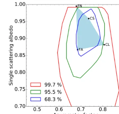
single-Figure 3.Example of a region (light-blue area) in the{g, ω0}
solu-tion space at 0.44 µm defined by four aerosol vertices: single fine-mode non-absorbing (FN), single fine-fine-mode absorbing (FA), coarse mode with small radius (CS) and coarse mode with large radius (CL). The isolines show the probability that the aerosol single-scattering properties derived from AERONET observations with the method of Dubovik et al. (2006) fall within the delineated spaces.
scattering albedo and phase function values derived from AERONET observations acquired in a specific region of in-terest for a given period (Dubovik et al., 2006). The red iso-line in Fig. 3 deiso-lineates the area[g, ω0]of the solution space
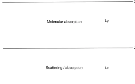
Figure 4. Atmospheric vertical structure of the FASTRE model. The surface is at levelZ0 and radiatively coupled with the lower
layerLaextending from levelZ0toZa. This layer includes
scatter-ing and absorption processes. The upper layer,Lg, runs from level ZatoZsand only accounts for gas absorption processes.
4 Forward radiative transfer model 4.1 Overview
The forward model, named FASTRE, simulates the TOA bidirectional reflectance factor (BRF)ym(x,b;m)as a func-tion of the independent parametersmdefining the observa-tion condiobserva-tions and a series of state variables x describing the state of the atmosphere and underlying surface. Model parametersbrepresent variables such as total column water vapour that influence the value ofym(x,b;m)but cannot be retrieved from the processed space-based observations due to the lack of information. The independent parameters m in-clude the illumination and viewing geometries(0, v)and the wavelength dependence. The RTE is solved with the ma-trix operator method (Fischer and Grassl, 1984) optimised by Liu and Ruprecht (1996) for a limited number of quadrature points.
The model simulates observations acquired within spec-tral bandseλcharacterised by their spectral response. Gaseous transmittances in these bands are precomputed and stored in LUTs. The model computes the contributions from sin-gle and multiple scattering separately, the latter being solved in Fourier space. In order to reduce the computation time, the forward model relies on the same atmospheric vertical struc-ture as in Govaerts et al. (2010b), i.e. a three-level system containing two layers (Fig. 4). The lowest level, Z0,
repre-sents the surface. The lower layer,La, ranging from levels Z0toZa, contains the aerosol particles. Molecular scattering and absorption also take place in that layer, which is radia-tively coupled with the surface for both single and the mul-tiple scattering. The upper layer,Lg, ranging fromZatoZs, is only subject to molecular absorption.
The surface reflectance rs(xs,b;m) over land is repre-sented by the so-called RPV (Rahman–Pinty–Verstraete)
model characterised by four parameters,xs= {ρ0, k, 2, ρc}, that are all wavelength dependent (Rahman et al., 1993). The
ρ0parameter, included in the [0,1] interval, controls the mean
amplitude of the BRF and strongly varies with wavelengths. Thekparameter is the modified Minnaert’s contribution that determines the bowl or bell shape of the BRF and typically varies between 0 and 2. The asymmetry parameter2of the Henyey–Greenstein phase function varies between−1 and 1. Theρcparameter controls the amplitude of the hotspot due to the “porosity” of the medium. This parameter varies between −1 and 1. For the simulations over the ocean, the Cox–Munk model (Cox and Munk, 1954) is used as implemented in Ver-mote et al. (1997).
Aerosol single-scattering properties in the layer La are represented by an external mixture of a series of predefined aerosol vertices as explained in Sect. 4.2. TheLg layer only contains absorbing gas not included in the scattering layer, such as high-altitude ozone, the part of the total column wa-ter vapour not included in layerLa and a few well-mixed gases.
The FASTRE model expresses the TOA BRF in a given spectral bandeλas a sum of the single I
↑
s and multipleI
↑
m
scattering contributions as in
ym(x,b;m)=TLg(b;m)
Is↑(x,b;m)+I
↑
m(x,b;m)
E0↓(m)µ0
, (1)
where
– Is↑(x,b;m)is the upward radiance field at levelZadue to the single scattering,
– Im↑(x,b;m)is the upward radiance field at levelZadue to the multiple scattering,
– TLg(b;m) denotes the total transmission factor in the Lglayer,
– E0↓(m)denotes the solar irradiance at levelZscorrected for the Sun–Earth distance variations.
The single-scattering contribution is written
Is↑(x,b;m)=
E0↓(m)µ0
π exp
−τ La µ0
rs(xs,b;m)exp
−τ La µv
, (2) whereτLa is the total optical thickness of layerLa.µ0and µvare the cosine of the illumination and viewing zenith
an-gles respectively.
The multiple-scattering contribution, Im↑(x,b;m), is
solved in the Fourier space for all illumination and viewing directions of the quadrature directions Nθ for 2Nθ−1 az-imuthal directions. The contributionIm↑(x,b;m)in the
4.2 Scattering layerLaproperties
The layer La contains a set of mono-mode aerosol mod-els v characterised by their single-scattering properties, i.e. the single-scattering albedo ω0,v(eλ)and phase function 8v(eλ, g)wheregrepresents the scattering angle. The dif-ferent vertices are combined into this layer according to their respective optical thicknessτv(eλ)with the total aerosol opti-cal thicknessτa(eλ)of the layer being equal to
τa(eλ)= X
v
τv(eλ). (3)
The phase function8v(eλ, g)is characterised by a limited numberNκ of Legendre coefficients equal to 2Nθ−1. The decision to use this number results from a trade-off between accuracy and computational time. WhenNκis too small, the last Legendre moment is often not equal to zero and the delta-M approximation is applied (Wiscombe, 1977). In this case, the αd coefficient of the delta-M approximation is equal to 8v(Nκ). The Legendre coefficientsκjbecome
cj= κj−αd
1−αd
, (4)
and the truncated phase function is denoted by80v. The cor-rected optical thickness τv0(eλ) and single-scattering albedo ω00,v(eλ)of the corresponding aerosol model become τv0(eλ)=(1−ω0,vαd)τv(eλ) (5) and
ω00,v(eλ)=
1−αd 1−ω0,vαd
ω0,v(eλ). (6)
The layer total optical thickness, τLa, is the sum of the gaseous,τg, the aerosol,τa0and the Rayleigh,τr, optical depth
τLa(eλ)=τg(eλ)+τa0(eλ)+τr(eλ), (7) with τa0(eλ)=
P vτ
0
v(eλ). The single-scattering albedo of the scattering layer is equal to
ω00(eλ)= P
cω00,v(eλ)τv0(eλ) τ0
a(eλ)
(8) and the layer average phase function
80(eλ, g)= P
c8 0
v(eλ, g)τv0(eλ) τ0
a(eλ)
. (9)
4.3 Gaseous layer properties
It is assumed that only molecular absorption takes place in layerLg. The height of levelZais used to partition the total column water vapour and ozone concentration in each layer assuming a US76 standard atmosphere vertical profile. This height is not retrieved and is therefore a model parameter of FASTRE, which should be derived from some climatological values.TLgdenotes the total transmission of that layer.
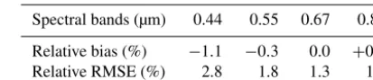
Table 1.Relative bias and root mean square error in percentage between FASTRE and the reference RTM in various spectral bands.
Spectral bands (µm) 0.44 0.55 0.67 0.87
Relative bias (%) −1.1 −0.3 0.0 +0.3
Relative RMSE (%) 2.8 1.8 1.3 1.2
4.4 FASTRE model accuracy
The simple atmospheric vertical structure composed of two layers is the principal assumption of the FASTRE model. In order to evaluate the accuracy of FASTRE, a similar proce-dure to that in Govaerts et al. (2010b) has been applied. The outcome of FASTRE has been evaluated against a more elab-orated 1-D radiative transfer model (RTM) (Govaerts, 2006) for sun and viewing angles varying from 0 to 70◦, for var-ious types of aerosols, surface reflectance and total column water vapour values. This reference RTM represents the ver-tical structure of the atmosphere with 50 layers. The mean relative bias and relative root mean square error (RMSE) be-tween the reference model and FASTRE have been estimated in the main spectral bands used for aerosol retrievals. The rel-ative RMSE,Rr, is estimated as
Rr=
v u u t 1
N X
N
ym(x,b;m)−yr(x,b;r)
yr(x,b;r)
2
, (10)
whereyr(x,b;m)is the TOA BRF calculated with the
ref-erence model. In this paper, the FASTRE model solves the RTE using 16 quadrature pointsNθ, which provides a good compromise between speed and accuracy. Results are shown in Table 1. The relative RMSE between FASTRE and the reference model is typically in the range of 1 %–3 %. An-other comparison of FASTRE has been made against actual Project for On-Board Autonomy-Vegetation (PROBA-V) ob-servations (Luffarelli et al., 2017). These comparisons show an RMSE in the range [0.024–0.038].
5 Inversion process 5.1 Overview
Surface reflectance characterisation requires multi-angular observationsy
e
scattering termIm↑(x,b;m)needs to be estimated only once
per spectral band. In the latter case, atmospheric properties cannot be assumed to be invariant and the multiple scattering contribution needs to be solved for each observation. When geostationary observations are processed, the accumulation period is often reduced to 1 day, and the assumption that the atmosphere does not change can be converted into an equiva-lent radiometric uncertainty (Govaerts et al., 2010b). Strictly speaking, it should be assumed that atmospheric properties have changed when the accumulation time exceeds several minutes (Luffarelli et al., 2016).
The retrieved state variables in each spectral bandeλ are composed of thexsparameters characterising the state of the surface and the set of aerosol optical thicknessesτvfor the aerosol vertices that are mixed in layer La. Prior informa-tion consists of the expected valuesxbof the state variables xcharacterising the surface and the atmosphere on one side, and regularisation of the spectral and/or temporal variability ofτvon the other side. Uncertainty matricesSxare assigned to this prior information. Finally, uncertainties in the mea-surements Sy are assumed to be normally distributed with zero mean. The inversion process of the FASTRE model will be herein referred to as the Combined Inversion of Surface and AeRosol (CISAR) algorithm.
5.2 Cost function
The fundamental principle of OE is to maximise the proba-bilityP =P (x|y
e
3,xb,b)with respect to the values of the state vectorx, conditional to the value of the measurements and any prior information. The conditional probability takes on the quadratic form (Rodgers, 2000):
P (x)∝exp h
− ym(x,b;m)−y
e
3 T
S−y1 ym(x,b;m)−y
e
3 i
+
exph−x−xbTS−x1 x−xb i
+
exph−xTHTaS−a1Hax i
+
exph−xTHTl S−l 1Hlx i
, (11)
where the first two terms represent weighted deviations from measurements and the prior state parameters respectively, the third represents the AOT temporal smoothness constraints and the fourth represents the AOT spectral constraint, with respective uncertainty matricesSaandSl. The algorithm pro-posed by Dubovik et al. (2011) implements similar temporal and spectral smoothness constraints. The two matrices Ha andHl, representing respectively the temporal and spectral constraints, can be written as block diagonal matrices:
H=
Hρ0 0 0 0 0
0 Hk 0 0 0
0 0 Hθ 0 0
0 0 0 Hρc 0
0 0 0 0 Hτ
, (12)
where the four blocksHρ0,Hk,HθandHρcexpress the
spec-tral constraints between the surface parameters. Their values are set to zero when these constraints are not active. The sub-matrixHτa can also be written using blocksHτ
a;eλ,v
along the diagonal. For a given spectral bandeλand aerosol vertexv, the blockHτ
a;eλ,v
is defined as follows:
Hτ a;eλ,v
τ eλ,v =
1 −1 0 . . . . 0 1 −1 0 . . . . . . . . . . 1 −1 . . . 0
τ
eλ,v,1
τ
eλ,v,2
. . . τ
eλ,v,Nt−1
τ
eλ,v,1,Nt
. (13) In the same way, the submatrixHτl can be written using blocksHτl;v,t. For a given aerosol vertex v and timet, the blockHτl;v,tis defined as follows:
Hτl;v,tτv,t=
0 0 0 . . . 0
−21 1 0 . . . 0
0 −3
2 1 . . . 0
. . . .. 0 . . . −Nλ
Nλ−1 1
τ1,v,t
τ2,v,t
τ3,v,t
. . . τNeλ,v,t
, (14)
where thelrepresents the uncertainties associated with the AOT spectral constraints of the individual vertexv, bound-ing the solution space. The spectral variations ofτvbetween bandeλlandeλl+1are assumed to vary, as
τ
eλl,v τeλ
l+1,v
= eeλl eeλ
l+1
, (15)
wheree
eλl is the extinction coefficient in bandeλl.
Maximising the probability function in Eq. (11) is equiva-lent to minimising the negative logarithm
J (x)=Jy(x)+Jx(x)+Ja(x)+Jl(x), (16) with
Jy(x)= ym(x,b, )−ye3
S−y1 ym(x,b, )−ye3
T (17)
Jx(x)= x−xbS−x1 x−xbT (18) Ja(x)=xTHTaS
−1
a Hax (19)
Jl(x)=xTHTl S −1
l Hlx. (20)
the variance should decrease. Accordingly, the magnitude of the elements of the covariance matrix should decrease as 1/√ny. Thus, repeating similar observations results in some enhancements of retrieval accuracy, which is proportional to the ratio ny/nx. Hence, the cost function which is actually minimised isJs(x)=Jy(x)+ny/nx(Jx(x)+Ja(x)+Jl(x)). 5.3 Retrieval uncertainty estimation
The retrieval uncertainty is based on the OE theory, assuming linear behaviour ofym(x,b;m)in the vicinity of the solution
ˆ
x. Under this condition, the retrieval uncertaintyσˆxis deter-mined by the shape ofJ (x)atxˆ
σxˆ2= ∂2J
s(x) ∂x2
−1 =
KTxS−y1Kx+S−x1+HTaS −1
a Ha+HTl S −1
l Hl −1
, (21) whereKx is the Jacobian matrix ofym(x,b;m)calculated inx. Combining Eqs. (21) and (8), the uncertainty in the re-ˆ trieval ofω0in bandeλis written
σω2ˆ 0(eλ)=
X
v
ω0,v(eλ)−ω0(eλ) τa(eλ)
2 στ2ˆ
v(eλ). (22) A similar equation can be derived for the estimation ofσg2. 5.4 Acceleration methods
The minimisation of Eq. (16) relies on an iterative approach withym(x,b;m)and the associated JacobiansKx being es-timated at each iteration. In order to reduce the calculation time dedicated to the estimation ofym(x,b;m)andKx, a se-ries of methods have been implemented. All quantities that do not explicitly depend on the state variables, such as the observation conditions m, model parameters b, quadrature point weights, etc. are computed only once prior to the opti-misation.
When solving the RTE, the estimation of the multiple scat-tering term is by far the most time-consuming step. Hence, during the iterative optimisation process, when the change
1τa(eλ)between iterationj andj+1 is small, the multiple scattering contribution at iterationj+1 is estimated with
Im↑(τa(j+1,eλ),b;m)=Im↑(τa(j,eλ),b;m) +∂I
↑
m(τa(j,eλ),b;m) ∂τa
1τa(eλ). (23)
This approximation is not used in two successive iterations to avoid inaccurate results, and the single-scattering contri-bution is always explicitly estimated.
6 Algorithm performance evaluation 6.1 Experimental set-up
A simple experimental set-up based on simulated data has been defined to illustrate the performance of the CISAR al-gorithm as a function of the chosen solution space. More specifically, the capability of CISAR to continuously sample the{g, ω0}solution space is examined in detail. For the sake
of simplicity, a noise-free multi-angular observation vector, y
e
3, where expresses the illumination and viewing ge-ometries, is assumed to be acquired instantaneously in the principal plane and in the spectral bands listed in Table 1. A radiometric uncertainty of 3 % is assumed to composeSy. In this ideal configuration, the solar zenith angle (SZA) is set to 30◦. In these experiments, to concentrate on the retrieval of aerosol properties, the surface parameters prior values are set to the true values used in the simulation (Table 5) with an ascribed uncertainty of 0.03. The first guess values are ran-domly chosen within this uncertainty interval. Part 2 explains how prior information on the surface parameters can be de-rived. No prior information is assumed for the aerosol optical thickness; i.e. the prior uncertainty is set to very large values. Only regularisation of the spectral variations ofτais applied. The CISAR algorithm performance evaluation is based on a series of experiments corresponding to different selec-tions of aerosol properties, both for the forward simulation of the observations and their inversion. Three different aerosol models are used in the forward simulations: F0, which only contains fine-mode; F1, which contains a dual-mode particle size distribution dominated by small particles; and F2, com-posed of a dual-mode distribution dominated by the coarse particles. Table 2 contains the values of the size distribution and refractive indices of these aerosol models. Values for the four vertices (FA, FN, CL and CS) enclosing the solution space as illustrated in Fig. 3 are given in Table 3. When the observations simulated with aerosol types F0, F1 or F2 are inverted, the list of vertices actually used depends on the type of experiment as indicated in Table 4. For all these scenarios, an AOT of 0.4 at 0.55 µm is assumed.
Values used for the RPV parameters in the four selected bands are indicated in Table 5. They correspond to typical BRF values that would be observed over a vegetated surface with a leaf area index value of 3 and a bright underlying soil. 6.2 Results
6.2.1 Experiment F00
Table 2.List of aerosol properties used for the simulations. The parametersrmfandrmcare the median fine- and coarse-mode radii expressed
in µm. Their respective standard deviations areσrmfandσrmc. The parametersnrandniare the real and imaginary part of the refractive index in the indicated bands.NfandNcare the fine- and coarse-mode particle concentration in number of particles per cm3.
Centre band in µm 0.44 0.55 0.67 0.87
Type rmf rmc ni nr nr nr Nf Nc
F0 0.08 – 1.396 1.393 1.391 1.388 – –
F1 0.10 0.93 1.419 1.427 1.436 1.442 9.587 0.002 F2 0.08 0.77 1.498 1.520 1.544 1.542 8.975 0.024
σrmf σrmc ni ni ni ni
F0 0.45 – 0.012 0.012 0.012 0.012 – –
F1 0.43 0.62 0.006 0.005 0.005 0.005 F2 0.50 0.62 0.005 0.005 0.004 0.004
Table 3.Microphysical parameter values for the four vertices (FA, FN, CS and CL) in the selected spectral bands. Radius are given in µm.
Centre band in µm 0.44 0.55 0.67 0.87 0.44 0.55 0.67 0.87
Type rm σrm nr nr nr nr ni ni ni ni
FN 0.08 0.45 1.3958 1.3932 1.3909 1.3879 0.0006 0.0006 0.0006 0.0006 FA 0.08 0.45 1.3958 1.3932 1.3909 1.3879 0.0207 0.0207 0.0207 0.0205 CS 0.30 0.55 1.4889 1.4878 1.4845 1.4763 0.0029 0.0029 0.0029 0.0029 CL 1.00 0.55 1.4889 1.4878 1.4845 1.4763 0.0029 0.0029 0.0029 0.0029
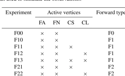
Table 4.List of experiments: the names are provided in the first column. The active vertices in each experiment are indicated with the ×symbol. The last column indicates the name of the aerosol model used to simulate the observations.
Experiment Active vertices Forward type
FA FN CS CL
F00 × × F0
F10 × × F1
F11 × × × F1
F12 × × × F1
F13 × × × × F1
F21 × × × F2
F22 × × × F2
F23 × × × × F2
as for the FN and FA vertices used for the inversion. Hence, the retrieval is limited to the imaginary part of the index of refraction, the real part being set to 1.4. With a retrieval con-figuration restricted to the use of only two vertices, the so-lution space for each wavelength is limited to a straight line between the two vertices.
Results are shown in Fig. 5 for the atmosphere and Table 5 for the surface. The asymmetry factorgand single-scattering albedoω0 are almost exactly retrieved. There is practically
no uncertainty in the retrieval ofgbecause of the constraints imposed by the fact that the particle radius is the same as for
the F0 aerosol model. The retrieved AOT is also in very good agreement with the true values as can be seen on the right panel. The retrieval errorτ is defined as the difference be-tween the retrieved and the true AOT values. Results are sum-marised in Table 6. This first experiment demonstrates that it is possible to retrieve the properties of the aerosol model F0 as a linear combination of the vertices FA and FN when only the absorption varies, the particle median radius being con-stant.
A comparison between the true and retrieved values in Ta-ble 5 shows that the surface parameters are very accurately retrieved. As stated in Sect. 6.1, prior information on the magnitude of the RPV parameter is assumed to be unbiased with an uncertainty of 0.03. The corresponding posterior un-certainties exhibit a significant decrease for theρ0
Table 5.Values of the true and retrieved surface RPV parameters for experiment F00. Wavelengths are given in µm.
True Retrieved
Band ρ0 k 2 ρc ρ0 k 2 ρc
0.44 0.025 0.666 −0.150 0.125 0.025±0.006 0.666±0.030 −0.150±0.030 0.125±0.030 0.55 0.047 0.657 −0.114 0.023 0.047±0.004 0.657±0.029 −0.116±0.028 0.023±0.030 0.67 0.056 0.710 −0.096 0.025 0.056±0.004 0.711±0.028 −0.096±0.026 0.025±0.030 0.87 0.238 0.706 −0.019 0.030 0.238±0.011 0.705±0.025 −0.020±0.017 0.029±0.030
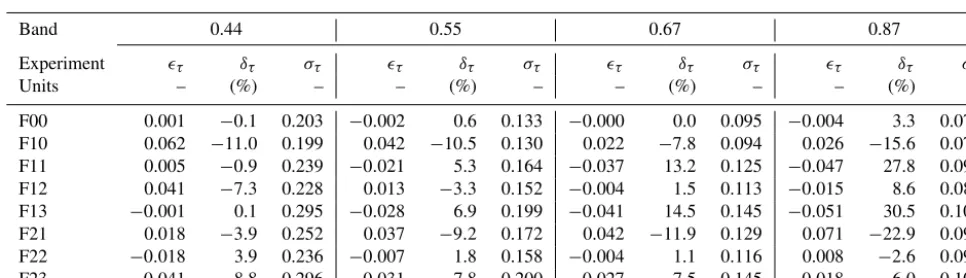
Table 6.Retrieved AOT error and uncertainties for the six experiments. The errorτis calculated as the difference between the retrieved and the true values,δτis the relative error in percent andστis the retrieval uncertainty estimated with Eq. (21). Wavelengths are given in µm.
Band 0.44 0.55 0.67 0.87
Experiment τ δτ στ τ δτ στ τ δτ στ τ δτ στ
Units – (%) – – (%) – – (%) – – (%) –
F00 0.001 −0.1 0.203 −0.002 0.6 0.133 −0.000 0.0 0.095 −0.004 3.3 0.079
F10 0.062 −11.0 0.199 0.042 −10.5 0.130 0.022 −7.8 0.094 0.026 −15.6 0.078 F11 0.005 −0.9 0.239 −0.021 5.3 0.164 −0.037 13.2 0.125 −0.047 27.8 0.095
F12 0.041 −7.3 0.228 0.013 −3.3 0.152 −0.004 1.5 0.113 −0.015 8.6 0.089
F13 −0.001 0.1 0.295 −0.028 6.9 0.199 −0.041 14.5 0.145 −0.051 30.5 0.103 F21 0.018 −3.9 0.252 0.037 −9.2 0.172 0.042 −11.9 0.129 0.071 −22.9 0.096
F22 −0.018 3.9 0.236 −0.007 1.8 0.158 −0.004 1.1 0.116 0.008 −2.6 0.090
F23 −0.041 8.8 0.296 −0.031 7.8 0.200 −0.027 7.5 0.145 −0.018 6.0 0.103
retrieval exhibits very similar behaviour for the other experi-ments and will not be shown.
6.2.2 Experiment F10
Let us now examine the case in which bothrmandni differ from those of the vertices used for the inversion. The aerosol type F1 is used for the forward simulation withrmf=0.1 µm
for the predominant fine mode and rmc=0.93 µm for the
coarse mode. The same aerosol vertices as in experiments F00 are used for the inversion.
The results in Fig. 6 show that ω0is reasonably well
re-trieved unlike thegparameter, which is systematically under-estimated. At any given wavelengths, it is not possible to re-trievegvalues outside the bounds defined by the FA and FN vertices. Consequently, the retrieved AOT values are under-estimated by about 10 % (Table 6). This example illustrates the retrieval failure when the actual solution lays outside the {g, ω0}space defined by the active vertices.
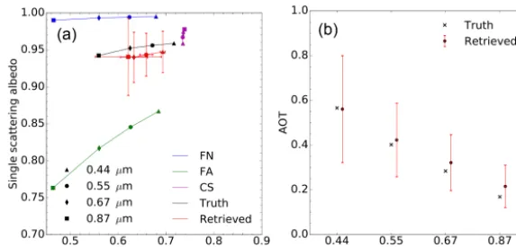
6.2.3 Experiments F11–F13
In order to improve the retrieval of the F1 aerosol model properties, the additional aerosol CS vertex withrm=0.3 µm
has been added for the inversion process. Results of exper-iment F11 are displayed in Fig. 7. Retrieved g values are no longer underestimated. The single-scattering albedo is slightly underestimated. It should be noted that the estimated uncertainty associated withgincreases with wavelength and
is particularly large at 0.87 µm, but rather underestimated at 0.44 µm. The improvement in the AOT retrieval accuracy is noticeable in the 0.44 and 0.55 µm bands where the magni-tude ofr is reduced from 0.062 to 0.005 and from 0.042
to−0.021 respectively (Table 6). At larger wavelengths, the benefit of adding the CS vertex is less noticeable though the magnitude ofrremains below 0.05. Finally, the retrieval
un-certainty slightly increases from 0.199 up to 0.239 for the 0.44 µm band because of the use of additional state variables
τvassociated with the inclusion of an additional vertex. Sim-ilar behaviour is observed in the other bands.
For experiment F12, the CS vertex is substituted by vertex CL which has a median radius of 1.0 µm. The use of this ver-tex instead of CS considerably improves the retrieval ofgand ofω0at large wavelengths (Fig. 8). As can be seen in Fig. 2,
the sensitivity of aerosol single-scattering properties to parti-cle median radius and imaginary part of the refractive index depends on the wavelength. Hence, a similar performance of the algorithm at all wavelengths should not be expected. The errorsτ in this experiment F12 are further reduced com-pared to experiment F11 with the exception of the 0.44 µm band. The CISAR algorithm retrieves total AODs consistent with the truth.
Finally, in experiment F13 the inversion was performed using all four vertices (Fig. 9). This additional “degree of freedom” translates into an increase of the estimated uncer-taintyστˆ as a result of the large number of possible way to
Figure 5. (a)Results of experiment F00 in the{g, ω0}space. The aerosol vertices used for the inversion are FN (blue) and FA (green). The
forward aerosol properties are shown in black and the retrieved ones in red. Vertical and horizontal red bars indicate the uncertainty of the retrieved values.(b)Retrieved AOT (red circles). The retrieval uncertainty is shown with the vertical red lines. True values are indicated with black crosses. True and retrieved values are slightly staggered to ease the reading.
Figure 6.Same as Fig. 5 but for experiment F10.
aerosol model F1. In other words, using these two coarse mode vertices does not improve the characterisation of F1. The actual benefit of adding this fourth vertex, i.e. expand-ing the solution space, is therefore not straightforward, and it should be noted that increasing the number of vertices im-pacts the computational time. This series of experiments has shown that, of the four considered, the use of the FN, FA and CL vertices provides the best combination for the retrieval of aerosol model F1. With this combination, the FN and FA vertices allow for control of the amount of radiation absorbed by the aerosols, while the effects of the particle size are con-trolled by the CL vertex.
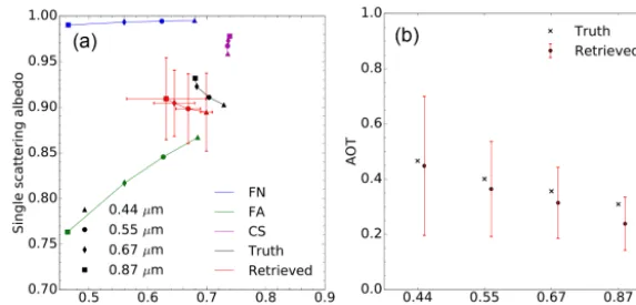
6.2.4 Experiments F21–F23
The retrieval of aerosol model F2, a dual-mode particle size distribution dominated by coarse particles, is now exam-ined. This model is composed of a fine mode with radius
rmf=0.08 µm and a coarse mode with radiusrmc=0.77 µm.
As for the retrieval of the F1 aerosol model, three combina-tions of vertices have been explored, i.e. FN, FA and CS for experiment F21 (Fig. 10), FN, FA and CL for experiment
F23 (Fig. 11) and FN, FA, CS and CL for experiment F22 (Fig. 11). Essentially the same conclusions hold as for the retrieval of aerosol model F1. The retrieval of the F2 model properties expressed as a linear combination of the FN, FA and CL vertices provides the best solution, with bothgand
ω0being retrieved at all wavelengths.
7 Discussion and conclusion
Figure 7.Same as Fig. 5 but for experiment F11.
Figure 8.Same as Fig. 5 but for experiment F12.
Figure 10.Same as Fig. 5 but for experiment F21.
Figure 11.Same as Fig. 5 but for experiment F22.
A fast-forward radiative transfer model has been designed which solves the radiative transfer equation without relying on precomputed look-up tables. This model considers two at-mospheric layers. The upper layer only hosts molecular ab-sorption. The lower layer accounts for both absorption and scattering processes due to aerosols and molecules and is ra-diatively coupled with the surface represented with the RPV BRF model. Single-scattering aerosol properties in this layer are expressed as a linear combination of the properties of ver-tices enclosing part of the solution space.
A series of different experiments has been devised to anal-yse the behaviour of the CISAR algorithm and its capability to retrieve aerosol single-scattering properties as well as the optical thickness. This discussion focuses on the retrieval of aerosol models dominated by the fine mode or coarse mode. These two models have pretty different spectral behaviour in the{g, ω0}space and yet the CISAR algorithm is capable of
retrieving the corresponding single-scattering properties in both cases with estimated uncertainties of about 15 %.
These experiments illustrate the possibility of using Eqs. (8) and (9) for the continuous retrieval of the aerosol single-scattering albedo and phase function. These equations assume linear behaviour of ω0 andg in the solution space.
Such assumptions have proven to be valid for the case ad-dressed in experiment F00. This assumption is not exactly true for the retrieval aerosol models of a fine- and a coarse-particle size modes. However, the retrieved aerosol single-scattering properties are derived much more accurately than with a method based on a limited number of predefined aerosol models as in Govaerts et al. (2010b), where the single-scattering properties of only predefined models are re-trieved. It thus represents a major improvement with respect to these types of retrieval approaches without requiring the use of a large number of state variables as in the method pro-posed by Dubovik et al. (2011), where aerosol microphysical properties are explicitly included in the set of retrieved state variables.
The choice of vertices outlining the{g, ω0}solution space
is critical. In these experiments, the best retrieval is ob-tained using three vertices, i.e. one vertex composed of small weakly absorbing particles (FN), one vertex composed of small absorbing particles (FA) and one vertex composed of large particles (CL). The use of a fourth vertex (CS) does not improve the retrieval and increases the estimated retrieval un-certainty.
This set of experiments represents ideal conditions, i.e. noise-free observations in the principal plane with no bias on the surface prior. This choice is motivated by the need to keep the result interpretation simple to illustrate how the new retrieval concept developed in this paper works. These experiments show the possibility of retrieving aerosol single-scattering properties within the solution space provided it is correctly bounded by the vertices. It is clear that adding noise to the observations will degrade the quality of the retrieval. Similar conclusions can hold if the observations are taking
place far from the principal plane, where most of the angular variations occur. Part 2 addresses the performance of CISAR when applied to actual satellite data.
Data availability. Results presented in Sect. 6 are available from the authors upon request.
Supplement. It includes the plots of case F22, adding a 3 % Gaussian noise to the simulated TOA BRF for AOT=0.05 (Fig. S1), AOT=0.2 (Fig. S2), AOT=0.4 (Fig. S3) and AOT=0.8 (Fig. S4). Figure S5 shows the merged results in the{g, ω0}
space of experiments F11, F12 and F13. Figure S6 shows the merged results in the{g, ω0}space of experiments F21, F22 and
F23. The supplement related to this article is available online at: https://doi.org/10.5194/amt-11-6589-2018-supplement.
Author contributions. YG developed the FASTRE model, con-ceived the experimental set-up and wrote the paper. ML contributed to the development of the inversion method.
Competing interests. The authors declare that they have no conflict of interest.
Acknowledgements. The authors would like to thank the reviewers for their fruitful suggestions.
Edited by: Andrew Sayer
Reviewed by: three anonymous referees
References
Cox, C. and Munk, W.: Measurement of the Roughness of the Sea Surface from Photographs of the Sun’s Glitter, J. Opt. Soc. Am., 44, 838–850, https://doi.org/10.1364/JOSA.44.000838, 1954. Diner, D. J., Hodos, R. A., Davis, A. B., Garay, M. J.,
Mar-tonchik, J. V., Sanghavi, S. V., von Allmen, P., Kokhanovsky, A. A., and Zhai, P.: An optimization approach for aerosol re-trievals using simulated MISR radiances, Atmos. Res., 116, 1– 14, https://doi.org/10.1016/j.atmosres.2011.05.020, 2012. Dubovik, O., Sinyuk, A., Lapyonok, T., Holben, B. N., Mishchenko,
M., Yang, P., Eck, T. F., Volten, H., Munoz, O., Veihelmann, B., van der Zande, W. J., Leon, J. F., Sorokin, M., and Slutsker, I.: Application of spheroid models to account for aerosol particle nonsphericity in remote sensing of desert dust, J. Geophys. Res.-Atmos., 111, 11208–11208, 2006.
Fischer, J. and Grassl, H.: Radiative transfer in an atmosphere-ocean system: an azimuthally dependent matrix-operator ap-proach, Appl. Optics, 23, 1032–1039, 1984.
Govaerts, Y. and Lattanzio, A.: Retrieval Error Esti-mation of Surface Albedo Derived from Geostation-ary Large Band Satellite Observations: Application to Meteosat-2 and -7 Data, J. Geophys. Res., 112, D05102, https://doi.org/10.1029/2006JD007313, 2007.
Govaerts, Y., Luffarelli, M., and Damman, A.: Effects of Sky Ra-diation on Surface Reflectance: Implications on The Derivation of LER from BRF for the Processing of Sentinel-4 Observations, in: Living Planet Symposium 2016, 9–13 May, Prague, Czech Republic, 2016.
Govaerts, Y. M.: RTMOM V0B.10 User’s Manual, 2006.
Govaerts, Y. M., Lattanzio, A., Taberner, M., and Pinty, B.: Generating global surface albedo products from multiple geo-stationary satellites, Remote Sens. Environ., 112, 2804–2816, https://doi.org/10.1016/j.rse.2008.01.012, 2008.
Govaerts, Y. M., Wagner, S., and Dubovik, O.: Enhanced retrieval of loading and detailed micro-physics of atmospheric aerosol from MTG/FCI observations, in: EUMETSAT Meteorological User Conference, 20–24 September, Córdoba, Spain, 2010a. Govaerts, Y. M., Wagner, S., Lattanzio, A., and Watts, P.: Joint
retrieval of surface reflectance and aerosol optical depth from MSG/SEVIRI observations with an optimal estimation approach: 1. Theory, J. Geophys. Res., 115, 10.1029/2009JD011779, https://doi.org/10.1029/2009JD011779, 2010b.
Hess, M., Koepke, P., and Schult, I.: Optical properties of aerosols and clouds: The software package OPAC, B. Am. Meteorol. Soc., 79, 831–844, 1998.
Kokhanovsky, A. A., Deuzé, J. L., Diner, D. J., Dubovik, O., Ducos, F., Emde, C., Garay, M. J., Grainger, R. G., Heckel, A., Herman, M., Katsev, I. L., Keller, J., Levy, R., North, P. R. J., Prikhach, A. S., Rozanov, V. V., Sayer, A. M., Ota, Y., Tanré, D., Thomas, G. E., and Zege, E. P.: The inter-comparison of major satellite aerosol retrieval algorithms using simulated intensity and polar-ization characteristics of reflected light, Atmos. Meas. Tech., 3, 909–932, https://doi.org/10.5194/amt-3-909-2010, 2010. Lattanzio, A., Schulz, J., Matthews, J., Okuyama, A., Theodore, B.,
Bates, J. J., Knapp, K. R., Kosaka, Y., and Schüller, L.: Land Sur-face Albedo from Geostationary Satelites: A Multiagency Col-laboration within SCOPE-CM, B. Am. Meteorol. Soc., 94, 205– 214, https://doi.org/10.1175/BAMS-D-11-00230.1, 2013. Liu, Q. and Ruprecht, E.: Radiative transfer model: matrix operator
method, Appl. Optics, 35, 4229–4237, 1996.
Luffarelli, M. and Govaerts, Y.: Joint retrieval of surface reflectance and aerosol properties with continuous variation of the state variables in the solution space: Part 2: Application to geosta-tionary and polar orbiting satellite observations, Atmos. Meas. Tech. Discuss., https://doi.org/10.5194/amt-2018-265, in review, 2018.
Luffarelli, M., Govaerts, Y., and Damman, A.: Assessing hourly aerosol properties retrieval from MSG/SEVIRI observations in the framework of aeroosl-cci2, in: Living Planet Symposium 2016, 9–13 May, Prague, Czech Republic, 2016.
Luffarelli, M., Govaerts, Y., Goossens, C., Wolters, E., and Swin-nen, E.: Joint retrieval of surface reflectance and aerosol prop-erties from PROBA-V observations, part I: algorithm perfor-mance evaluation, in: Proceedings of MultiTemp 2017, 27–29 June, Bruges, Belgium, 2017.
Manolis, I., Grabarnik, S., Caron, J., Bézy, J.-L., Loiselet, M., Betto, M., Barré, H., Mason, G., and Meynart, R.: The MetOp second generation 3MI instrument, Proc. SPIE Remote Sens., 88890J, https://doi.org/10.1117/12.2028662, 2013.
Marquardt, D.: An Algorithm for Least-Squares Estimation of Non-linear Parameters, SIAM J. Appl. Math., 11, 431–441, 1963. Pinty, B., Roveda, F., Verstraete, M. M., Gobron, N., Govaerts, Y.,
Martonchik, J. V., Diner, D. J., and Kahn, R. A.: Surface albedo retrieval from Meteosat: Part 1: Theory, J. Geophys. Res., 105, 18099–18112, 2000a.
Pinty, B., Roveda, F., Verstraete, M. M., Gobron, N., Govaerts, Y., Martonchik, J. V., Diner, D. J., and Kahn, R. A.: Surface albedo retrieval from Meteosat: Part 2: Applications, J. Geophys. Res., 105, 18113–18134, 2000b.
Rahman, H., Pinty, B., and Verstraete, M. M.: Coupled surface-atmosphere reflectance (CSAR) model, 2. Semiempirical surface model usable with NOAA Advanced Very High Resolution Ra-diometer Data, J. Geophys. Res., 98, 20791–20801, 1993. Rodgers, C. D.: Inverse methods for atmospheric sounding, Series
on Atmospheric Oceanic and Planetary Physics, World Scien-tific, Oxford, 2000.
Schuster, G. L., Dubovik, O., Holben, B. N., and Clothiaux, E. E.: Inferring black carbon content and specific absorption from Aerosol Robotic Network (AERONET) aerosol retrievals, J. Geophys. Res., 110, 1017–1017, 2005.
Serene, F. and Corcoral, N.: PARASOL and CALIPSO: Experi-ence Feedback on Operations of Micro and Small Satellites, in: SpaceOps 2006 Conference, 21 June, American Institute of Aeronautics and Astronautics, https://doi.org/10.2514/6.2006-5919, 2006.
Vermote, E. F., Tanré, D., Deuzé, J. L., Herman, M., and Morcrette, J. J.: Second simulation of the satellite signal in the solar spec-trum, 6S: An overview, IEEE T. Geosci. Remote, 35, 675–686, 1997.
Wagner, S. C., Govaerts, Y. M., and Lattanzio, A.: Joint retrieval of surface reflectance and aerosol optical depth from MSG/SEVIRI observations with an optimal estimation approach: 2. Imple-mentation and evaluation, J. Geophys. Res., 115, D02204, https://doi.org/10.1029/2009JD011780, 2010.