SECURE MULTIPARTY PROTOCOL FOR
DIFFERENTIALLY-PRIVATE DATA RELEASE
by Anthony Harris
A thesis
submitted in partial fulfillment
of the requirements for the degree of
Master of Science in Mathematics
Boise State University
© 2018
Anthony Harris
DEFENSE COMMITTEE AND FINAL READING APPROVALS
of the thesis submitted by Anthony Harris
Thesis Title: Secure Multiparty Protocol for Differentially-Private Data Release Date of Final Oral Examination: 12 March 2018
The following individuals read and discussed the thesis submitted by student Anthony Harris, and they evaluated the presentation and response to questions during the final oral examination. They found that the student passed the final oral examination.
Gaby Dagher, Ph.D. Chair, Supervisory Committee Liljana Babinkostova, Ph.D. Member, Supervisory Committee Marion Scheepers, Ph.D. Member, Supervisory Committee
I would like to thank the Mathematics Department for providing the opportunity to continue my education. I would also like to thank my advisor Dr.Dagher for introducing me to the field of cryptology and providing the foundation to pursue a Ph.D, as well as the committee members for their helpful feedback. Finally, I would like to thank my family and friends for their enduring support.
As I continued the Master’s program at Boise State University, my interests began to converge towards cryptology and digital privacy. As our world continues to advance in technology, society will need to place a higher emphasis on cyber security and privacy. I am grateful for dedicating my research in a fast-paced and dynamic field.
In the era where big data is the new norm, a higher emphasis has been placed on models which guarantees the release and exchange of data. The need for privacy-preserving data arose as more sophisticated data-mining techniques led to breaches of sensitive informa-tion. In this thesis, we present a secure multiparty protocol for the purpose of integrating multiple datasets simultaneously such that the contents of each dataset is not revealed to any of the data owners, and the contents of the integrated data do not compromise individual’s privacy. We utilize privacy by simulation to prove that the protocol is privacy-preserving, and we show that the output data satisfies-differential privacy.
Abstract . . . vi
List of Tables . . . x
List of Figures . . . xi
LIST OF ABBREVIATIONS . . . xii
LIST OF SYMBOLS . . . xiii
1 Introduction . . . 1
1.1 Motivation . . . 1
1.2 Challenges & Concerns . . . 2
1.3 Contributions . . . 3
1.4 Thesis Statement . . . 4
1.5 Organization of the Thesis . . . 4
2 Background . . . 5
2.1 Privacy & Security . . . 5
2.2 Cryptographic Primitives . . . 7
2.3 Privacy Model . . . 9
2.3.1 Exponential Mechanism . . . 11
2.3.2 Laplace Mechanism . . . 12
2.3.4 Information Gain . . . 14
2.4 Security Model . . . 17
2.4.1 Types of Security . . . 17
2.4.2 Computational Indistingushability . . . 18
2.4.3 Semi-honest Security . . . 21
3 Literature Review . . . 25
3.1 Privacy-preserving Data Processing . . . 26
3.2 Multiparty Privacy-preserving Data Publishing . . . 28
4 Secure Distributed Multiparty Exponential Mechanism . . . 31
4.1 Protocol Overview . . . 31
4.2 Protocol Details . . . 35
4.2.1 Indexing Attributes . . . 36
4.2.2 Indexing Attribute-Score Pairs . . . 37
4.2.3 Extended RVP & R-Shares . . . 37
4.2.4 L-Shares . . . 41
4.2.5 Selecting the Winning-Attribute . . . 42
4.2.6 Multiparty Exponential Mechanism Summary . . . 43
4.3 Protocol Analysis . . . 44
4.3.1 Security Analysis . . . 44
4.3.2 Complexity Analysis . . . 50
4.3.3 Correctness Analysis . . . 51
5 Secure Multiparty Protocol for Differentially-Private Data Release . . . 53
5.2 Protocol Details . . . 55
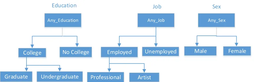
5.2.1 Attribute Taxonomy . . . 55
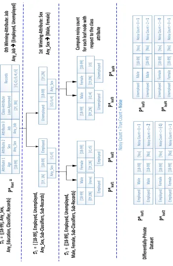
5.2.2 Partitioning Process . . . 61
5.2.3 Computing Count Vector . . . 67
5.2.4 Deriving the Encrypted True Count . . . 71
5.2.5 Deriving the Noisy Count . . . 75
5.2.6 Protocol Summary . . . 76
5.3 Protocol Analysis . . . 77
5.3.1 Security Analysis . . . 77
5.3.2 Complexity Analysis . . . 86
5.3.3 Correctness Analysis . . . 88
6 Conclusion . . . 92
6.1 Summary . . . 92
6.2 Future Work . . . 93
Bibliography . . . 94
2.1 Vertically-partitioned raw data owned by partiesP1,P2andP3 . . . 7
3.1 Comparison Table . . . 30
5.1 General TableT . . . 72
5.1 Attribute Taxonomies . . . 55 5.2 Partitioning Tree . . . 62
RVP– Random Value Protocol
MMC– Mix and Match Count Protocol
MAIN– Secure Multiparty Protocol for Differentially-Private Data Release Class,Cls– Classifier Attribute
Pj , denotes a party-member
Dj , denotes dataset owned by partyPj
D , collection of all datasets
ˆ
D , the integrated datasets Ai , denotes an attribute
Aw , denotes a winning attribute
JmK , denotes the encrypted version of messagem epsilon symbol, used as the privacy parameter
Rj , denotes the individual records owned by partyPj
φj Lowercase Phi symbol, denotes the set of attribute-score pairs {Ai} that party Pj owns
Φj Uppercase Phi symbol, denotes the set of attribute-score pairs{(Ai, Ui)}that party Pj owns
TAi , denotes the taxonomy of attributeAi
Tj , denotes the group taxonomy ofPj
T , denotes the intersected taxonomy of every attribute Pj∗ , denote partyPj’s sub-partitioning tree
P∗ , denotes a partitioning tree
S , denotes the number of specializations in the main algorithm ~
Vjk , denotes party-memberPj’skthattribute vector ~
Pj , denotes party-memberPj’s standardized attribute-vector ~
C , denotes the encrypted count-vector
T , denotes the Mix and Match Table c
≡ , denotes computational indistinguishability ~
x , denotes the list of initial inputs(x1, x2, . . . , xn)
Sj , denotes simulatorSj
f(~x) , denotes the ideal functional that takes~xas input
Π , Uppercase pi symbol, denotes a protocol
Chapter 1
INTRODUCTION
Recent technology has enabled both the size and storage of data to grow exponentially. Although data is abundant and widely available, it is advantageous for multiple data owners to integrate their respective data. By doing so, the integrated data becomes an enhanced version of the original distributed data, in terms of information and usability. This suggests cooperating parties have access to far better data compared to those working independently. For cooperation to exist, the parties must ensure that the integration protocol is both correct and privacy-preserving. Our protocol aims to establish a secure and private multiparty computation that allows for an efficient means of data integration.
1.1
Motivation
1.2
Challenges & Concerns
1.3
Contributions
Our main contribution involve deriving a protocol which securely integrates multiple datasets in a differentially-private fashion. This achievement is highlighted by the following:
• Creating an exponential mechanism that is applicable in multiparty setting. This process was achievable by the Multiparty Exponential Mechanism 4.1.
• Extending the functionality of the Random Value Protocol(RVP) [4] to be applicable in multiparty party setting, instead of a two-party setting.
• Creating a protocol that allows secure exchange of messages and computation among multiple users. This process was achievable through the Distributed Comparision 4.2. Distributed Comparison encodes and decodes messages through ElGamal encryption [37] and was designed to substitute the functionality of the Yao Protocol [20], which only offered secure computation in a two-party setting.
• Creating a protocol that allows a party to convert their records into binary-vectors with respect to one or more attributes. From there, the parties securely intersect their binary-vectors among themselves which is later used to create a differentially-private dataset. This process was made possible be the Secure & Private Attribute Counting Exchange 5.2 (SPACE) protocol. SPACE was designed to substitute the functionality of Secure Scalar Product Protocol [1], which is conceptually similar but only applicable in the two-party setting.
1.4
Thesis Statement
The objective of this thesis is to answer the following question: Given multiple data owners, how can they securely integrate their respective datasets such that the privacy is maintained and the output model is privacy-preserving?
Given multiple datasets D1, D2, . . . , Dn owned by P1, P2, . . . , Pn respectively, and a privacy budget, the goal of this thesis is to design a protocol that securely publishes an anonymized and integrated datasetDˆ for the purpose of statistical analysis such that: 1. The protocol is secure (privacy-preserving) in the semi-honest adversarial model. 2. The output is-differentially private.
1.5
Organization of the Thesis
This Thesis is organized as follows:
• Chapter 2 provides basic background knowledge which functions as the backbone of the thesis.
• Chapter 3 discusses relevant literature relating to secure computation, privacy, as well as various data publishing and data mining techniques.
• Chapter 4 discusses how the parties can securely derive a winning attributeAw in a differentially-private manner, using the Multiparty Exponential Mechanism 4.1.
• Chapter 5 will detail the main algorithm, where the parties collectively use Aw to securely derive a differentially-private datasetD.ˆ
Chapter 2
BACKGROUND
2.1
Privacy & Security
be compromised if their ’attribute-profile’ is too unique relative to other individuals in the dataset [25]. A common side-effect of large datasets is that the more attributes it acquires, the more unique and identifiable the individuals in the dataset become. To address this issue, we will employ differential-privacy as a means to protect the privacy of every individual in every dataset. An algorithm is said to be differentially private if by looking at the output, one cannot tell whether any individual’s data was included in the original dataset or not. In other words, a differentially private-algorithm guarantees that its outcome hardly changes when a single individual joins or leaves the dataset.
Beyond privacy we also want our protocol to be computationally secure. We have the option of having our protocol be secure with respect to one of the following models: honest, semi-honest, and malicious. For this thesis, we are only concerned with achieving security in the semi-honest setting. Semi-honest security assumes every party will follow the protocol exactly as described. As the parties conduct the protocol they will attempt to learn or reveal any information about the other participants. For a computation to be semi-honest secure, requires that no new information about any party is revealed or deduced during or after the execution of the protocol. A secure protocol requires the scheme to be mathematically secure prior to implementation.
Example 2.1.1. Imagine hospitalP1, health-insurance companyP2, and credit-card
com-panyP3all have distinct attributes.P1owns datasetD1 ={ID, Classif ier, Sex, Salary,R1},
P2ownsD2 ={ID, Classif ier, Education,R2}, andP3ownsD3 ={ID, Classif ier, J ob,R3},
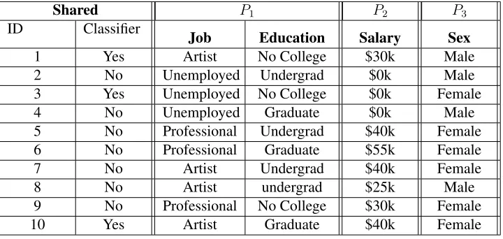
Table 2.1: Vertically-partitioned raw data owned by partiesP1,P2andP3
Shared P1 P2 P3
ID Classifier
Job Education Salary Sex
1 Yes Artist No College $30k Male
2 No Unemployed Undergrad $0k Male
3 Yes Unemployed No College $0k Female
4 No Unemployed Graduate $0k Male
5 No Professional Undergrad $40k Female
6 No Professional Graduate $55k Female
7 No Artist Undergrad $40k Female
8 No Artist undergrad $25k Male
9 No Professional No College $30k Female
10 Yes Artist Graduate $40k Female
Table 2.1, each column corresponds to a specific attribute, while each row corresponds to a single individual and their respective individual records. Notice individuals 1 and 4 have unique profiles, given that they are respectively the only author and lawyer within the dataset. This means individuals 1 and 4 are vulnerable linking attacks where by occupation alone the parities (or a data miner) can deduce their identities with absolute certainty, assuming the data in the dataset was sufficiently rich. To avoid attribute-based linking attacks, differential-privacy will be introduced later as a privacy measure.
2.2
Cryptographic Primitives
In this section we will detail all the encryption methods and mechanisms used throughout the thesis. These encryption methods were picked based on their versatility, specifically the ability to foster secure communication between two or more parties.
Exponential ElGamal [3]
of users. The encryption is both semantically secure and homomorphically additive. Each party uses their private keys jointly to encrypt and decrypt message m. The Exponential ElGamal sees the most amount of use during Protocol 4.2 (Distributed Comparison) and sees significant application in Protocol 5.2 (SPACE). For brevity, we denote the encryption of a message m as the ciphertext JmK. Given generatorg, prime p, group public-key A, group ephemeral-keyr, and public backdoorgr
JmK:= (A
r·gm mod p, gr mod p) (2.1)
There are many times within the paper when we mention “homomorphic addition”. Homo-morphic addition means that the “×” operator can be understood as the “+” operator. For instance we can homomorphically addaand bas follows ga×gb mod p = ga+b mode p. Homomorphic operations are consistently applied when dealing with ElGamal encryption. In a similar fashion, homomorphic encryption is described as follows:Ja+bK =JaK×JbK.
Random Value Protocol (RVP) [4]
RVP allows two parties to generate a random valueR, whereRhas been chosen uniformly within a predefined integer-based interval. This interval starts at 0 and ends at some positive integer-valueσ=σ1+σ2, whereR ∈[0, σ]. Ris not known by either party but it is shared
between them. More specifically, P1 hasR1 ∈ [0, σ1], and P2 hasR2 ∈ [0, σ2] whereσi
are both integers. R1 and R2 are considered random ’shares’ ofR, whereR = R1 +R2
and R, R1, R2 ∈ [0,P2i=1σi]. For the Multiparty Exponential Mechanism 4.1 RVP was generalized to includenparties.
Mix and Match [12]
the set as well as the multiplicity of their occurrence. However, the unique values and their respective multiplicities will remain encrypted throughout the scheme. The Mix and Match primitive is applied in Protocol 5.2.
Mix Network [13]
A mix network allows a list of encrypted messages to be jointly shuffled and re-encrypted such that no party knows the original arrangement of the encrypted messages. There are several ways of acquiring a mix network, where most require that each step to be verifiable by each of the party members. Mix network is applied in Protocol 5.2.
2.3
Privacy Model
In this section we introduce the notion of privacy. Typically, when people attempt to define privacy they do so holistically. But for the sake of consistency and correctness it is critical that privacy be defined mathematically. By doing so, there exists a consistent means of confirming or denying the privacy of a protocol. As to date, differential privacy is the”gold standard” of privacy. Differential privacy provides a well-defined, mathematical definition of privacy. This model makes no assumptions about the knowledge of an adversary. This ensures an adversary learns nothing new about an individual, whether or not their record is in the dataset [7].
Definition 2.3.1. -Differential Privacy: [7]
A randomized mechanismMis-differentially private if for all datasetsD1andD2(where
they differ at most one element), and for all possible anonymized dataset D.
A standard means to achieve differential privacy is to add random noise to the true output of the dataset. The noise is calibrated according to the sensitivity of the function. The sensitivity of a function is the maximum difference of its outputs from two datasets that differ only in one record. The sensitivity of a utility function is defined as follows
Definition 2.3.2. Sensitivity: [7]
For any functionf :D→R, the sensitivity off is
∆f = max
D1,D2
|f(D1)−f(D2)| (2.3)
For allD1,D2differing by at most one record.
Example 2.3.1. Imagine there are two datasets, D1 and D2. D1 contains the individual
records {A1, B1, C1, ..., Y1} with respect to an attribute and D2 contains the individual
records {A2, B2, C2, ..., Z2} with respect to another attribute. Notice D1 and D2 differ
by exactly one record. Since the two datasets are sufficiently close in size, sensitivity can be applied. Define functionf, which counts the elements in a given set.
∆f = max
D1,D2
|f(D1)−f(D2)|=|25−26|= 1
f described in this manner, is typically called the ’count function’. Howeverf is arbitrary
2.3.1 Exponential Mechanism
When implementing differential-privacy, it is typically done to numerical attributes where numerical noise is added to the dataset. By adding noise to the dataset, the privacy of each individual within the dataset is preserved. However, it is possible for Pj to own a dataset which contains numerical or categorical attributes. In the case of categorical attributes, it makes no sense to add noise directly. Luckily, there exists an ’exponential mechanism’ that achieves differential privacy whenever it makes no sense to add noise [24]. An exponential mechanism is a differentially private method to select an element from a set with high utility. The utility function u, takes dataset D ∈ Dn and takes some value A ∈ A as input, outputting a real value in return. Or in other words, u : (Dn × A) → R. For the utility function, a higher value corresponds to better data utility [24]. The exponential mechanism creates a probability distribution over the rangeA, where we then sample aa valueAi ∈ A[24]. For this paper,Dnrepresent the datasets among all parties,Arepresents the set of attributes among all parties, andu(D, A)returns utility-scoreU, whereDandA come from the same party. Our objective regarding the exponential mechanism is to create an(A, U)pair for all attributes, then probabilistically select anAwith high utility-score. Definition 2.3.3. Exponential Mechanism [7]:
For a set D, a set of possible outputs T, and scoring function U(D, t), privacy-budget > 0, a mechanism is an exponential mechanism if the probability of selectingt ∈ T is proportional to exp(·u2∆(D,tu )), where∆u = max
t,D1,D2
|u(D1, t)−u(D2, t)| and D1, D2 ∈ D
differ by at most one element.
mechanism correctly, then the protocol is-differentially private. Therefore if our protocol applies an exponential mechanism throughout some execution, then privacy is satisfied with respect to that execution.
2.3.2 Laplace Mechanism
Recall each party has a collection of both categorical and numerical attributes. Among all the parties we would like to probabilistically select a winning attribute Aw which has the highest utility. For our protocol, utility is loosely described relative to how unique the individuals are in Dj, with respect to one of Pj’s attribute. For instance, if Pj had the attributeA1which corresponds to job, where the majority of the individuals within thePj’s
dataset had the same job, thenA1would be assigned a low utility score. Conversely, if the
majority of the individuals in the dataset had different jobs, then A1 would be assigned
the noise is too large, the data becomes useless. Conversely, if the noise is too small, the privacy of the data is not preserved. The noise itself is derived from the Laplace random variable, whose distribution depend on the sensitivity of functionf.
Theorem 2.3.2. [26]
For any functionf :D →Rd, the mechanismM that adds independently generated noise with distribution Lap(∆f /) to each of thedoutputs satisfies-differential privacy.
Thus, as long as the appropriate amount of noise is added to the raw data prior to publishing, we can ensure that the integrated datasetDˆ is-differentially private.
2.3.3 Composition Theorems
What makes differentially privacy nice is that it allows compositions of several mechanism (or protocols), while keeping track of privacy. This allows us to keep track and tally the usage of our privacy budget, throughout the execution of the protocol. A privacy budget is a fixed value, usually denoted as. If there is a mechanism which requires some of the overall privacy budget (like0), then we would deduct some of the overall privacy budget (or what is currently available) by0. That being said we are never allowed to consume more of the privacy budget than we originally started with. There currently exist two well-known theorems which we will use later on in the paper to manage and keep track of our privacy budget.
Theorem 2.3.3. Sequential Composition [26]
Let each mechanism Mi provide i-differential privacy on dataset D. Then mechanism
M(M1, M2, . . . , Mn)provides(
Pn
Theorem 2.3.4. Parallel Composition [26]
Let each mechanismMi provide-differential privacy. Given a sequence ofMi(Di)over a set of disjoint datasets Di (i.e {M1(D1), M2(D2), . . . , Mn(Dn)}), where D = Sni=1Di
and∅=DaTDb for allDa, Db ∈D, as well as a mechanismM(M1, M2, . . . , Mn), then
Msatisfies max(i)-differential privacy.
2.3.4 Information Gain
In terms of an adequate utility function we recommend ’information gain’. Although there exists many utility functions to choose from. Information Gain (IG) takes a dataset and quantifies it based on how well it can be homogenized relative to a set of attributes and a classifier attribute. In this case, the set of attributes can be whatever you like (age, sex, weight, etc.). Similarity, a classifier attribute can also be arbitrary. What distinguishes the set of attributes from a classifier is that the set of attributes are used to predict the outcome of a classifier. For example, we can use the age, sex and weight of people within a dataset to predict whether someone (who is not in the dataset) has a bachelors degree or not. Doing this requires examining the ’entropy’ of each partition, relative to some attribute. A partition in this case refers to how the dataset is grouped or ”broken up” into smaller datasets, all of which consist of unique elements. For some partitionDkand dataset D, whereDk ⊆D, the entropy functionE is defined as follows
E(Dk) = − a
a+blog2( a a+b)−
b
a+blog2( b a+b)
whereais the number of individuals in partitionDkthat satisfies the classifier attribute and b is the number of individuals in partition Dk that do not satisfy the classifier attribute. Using entropy we can compute the information gain (IG) on dataset D with c many partitions such thatDi ⊂Dis defined as follows,
IG(D) =E(D)−
c
X
i=1
E(Di)
Typically, one can get many IG values depending on how the D is partitioned. Thus, the maximum IGvalue ofD normally takes priority. For numerical attributes, partitions are usually defined through a ’split point’. A split point is a value which splits a single set into two. For instance, consider the intervalI = [a, b], whereaandbare integers and a ≤ b. Assume there exists a split point c ∈ [a, b]. The original set I is now split into two, I1 = [a, c] andI2 = (c, b]. The contents of I1 and I2 will determine the respective
Example 2.3.2. Let us assume we have the following datasetD
ID AGE Education(classifier)
1 22 Yes
2 18 No
3 26 Yes
4 23 Yes
5 22 Yes
6 31 No
7 20 No
8 26 Yes
9 26 Yes
10 19 No
Notice datasetD contains the ”Age” attribute, which we will callA, along with the clas-sifier ”Education”. For this example let us assume the split point is t = 22. Given t, we partition A into two sets A1 and A2, where A1 contains the individuals that are 22
or older A1 = {1,3,4,5,6,8,9} and A2 contains the individuals that are younger than
22, A2 = {2,7,10}. We start by determining the entropy of attribute A as E(A) =
− 6 6+4log2(
6 6+4)−
4 6+4log2(
4
6+4) = 0.97095. Now we compute the entropy of each partition.
E(A1, t) = −6+16 log2(6+16 )− 6+11 log2(6+11 ) = 0.50167andE(A2, t)is assumed to be zero
since theA2 is perfectly homogenized relative to the classifier. Complete homogenization
of a dataset is assumed to have an entropy of 0. In general, any time we computelog2(0)
0.37928. If we assume that this information gain is maximum possible information among all possible split points, thenu(A, t) = 0.37928
2.4
Security Model
This section investigates the notion of security, both holistically and mathematically. We aim to investigate the concepts which will enable us to mathematically determine whether or not a particular protocol is secure or not.
2.4.1 Types of Security
If information is preserved throughout the duration of the execution, then the protocol is secure in the semi-honest setting. Finally, there are parties with malicious behavior. Malicious adversaries can essentially do as they want. They can deviate from the protocol, input false values, make no inputs at all, etc. Parties in the malicious-setting have the freedom to do whatever they feel like, given that the protocol does not have a mechanism to prevent deviant behavior. They will also attempt to learn new information about the participants throughout the execution of the protocol. A protocol is secure in the malicious setting if the protocol is both executable and does not leak any information, given that the parties will actively seek to deviate from the protocol. In this context, a protocol which is secure in the malicious case acquires the highest level of security. It may be possible to assume a variation of behaviors among different parties. For example, assume a protocol has three parties where one is honest and the other two are respectively semi-honest and malicious. In this case, the protocol could only be shown to be secure in the malicious setting. Security is hierarchal, where behavior of at least one party which corresponds to the highest security among all the parties will set the standard for security.
2.4.2 Computational Indistingushability
Our protocol is provably secure in semi-honest model for multiple parties. Semi-honest security relies on the concept of computational indistinguishability, where the information that Pi sends or receives cannot meaningfully be distinguished from the information that Pj sends or receives. In this section, we will highlight a few important mathematical components relevant to semi-honest security.
Definition 2.4.1. Computational Indistinguishability [19]
1 (heads) or 0 (tails). LetZ = z1z2. . . znbe the probability ensemble of the coin, where zi represents the outcome of theithcoin flip. Two probability ensemblesX andY can be assigned a computational distance through the following function.
|P r[D(X, ω) = 1∗]−P r[D(Y, ω) = 1∗]| (2.4)
where ω is the condition (or event) being tested and 1∗ is a boolean value that indicates whether the condition had successfully occurred. XandY are said to be computationally indistinguishable, or described equivalently asX ≡c Y, where for any function an efficient-algorithmD there exists a negligible functionepsilon(n) > 0, there exists some n > N such that
|P r[D(X, ω) = 1∗]−P r[D(Y, ω) = 1∗]|< (n) (2.5)
whereN ∈NandDis typically referred to as the ’distinguisher’
Example 2.4.1. The probability ensembles of X and Y are defined below, where we will assumeX represents a biased blue coin and Y represents a biased red coin. xi and yi represent the respective outcomes of each coin flip, where the value 1 designates an outcome of heads and 0 designates tails. In this scenario let us defineω1 as representing a
blue coin that outputs{1n}(all heads).
X(Blue) =
1
3 ifxi = 1 2
3 ifxi = 0
Y(Red) =
2
3 ifyi = 1 1
3 ifyi = 0
D(distinguisher) =
1∗(success) ifZ =ω1
0∗(f ailure) else
|P r[D(X, ω1) = 1∗]−P r[D(Y, ω1) = 1∗]|
=|(1
3)
n−0|
= (13)n
limn→∞(13)n= 0
Since the red coin can never yield a successful outcome (being blue, while having all heads), its respective probability is 0. The probability that the blue coin yields a successful output approaches zero as the number of coin flips increase, meaning the computational distance among the two coins becomes arbitrarily small. Although the computational distance in this instance is arbitrarily close , we cannot conclude thatX ≡c Y. Why?Xand Y can only be computationally indistinguishable if the computational distance is arbitrarily small foranydistinguisherD. We only showed the equation is satisfied with one specific distinguisher function. Establishing computational indistinguishability requires quite a bit of effort. For this example, a simple way of distinguishing the coins is by color. One could construct D2(Z, ω2), where ω2 represents a blue coin that acquires an outcome of heads
2.4.3 Semi-honest Security
The formalization of semi-honest security involves inserting a theoretical simulatorSj into protocol Π. The simulator wants to simulate communication between itself and Pj with respect to Π. Sj will communicate on the behalf of the other parties in such a manner that Pj will not be suspicious of Sj’s messages. In other words, the messages that Sj sends on the behalf of Pk (some other party not Pj) should be indistinguishable relative to whatPk would have actually sent. Another component we need to consider is a trusted third-party,f. The trusted third-party knows Πand all its operations with respect to each party. In an ideal setting, each partyPj will privately provide their initial-input xj to f. In returnf would privately reveal the final outputfj(~x) =fj(x1, x2, . . . , xn)toPj. In the literature,fis commonly referred to as the ’functionality’ within the ideal model. The ideal model differs significantly from the real model, where both models serve a distinct purpose. Within the real model, the parties conduct Π among each other, with an initial input of values. In the ideal model, parties are conductingΠ with either the trusted third-party or the simulator, given that each party has an initial set of inputs. When the parties computes
Πwith the trusted third-party, that can be loosely described as a perfectly secure procedure. If the final output in the real model is indistinguishable from the final output in the ideal modelandSj can properly simulate messages to Pj in an indistinguishable manner, then
Π will be deemed to be secure in the semi-honest setting [19]. The ideal model loosely represents an idealized execution ofΠ, with respect to security. If the ideal execution ofΠ
is indistinguishable from the real execution ofΠ, thenΠis secure. Prior to simulation Sj has access toPj’s initial inputxj, final outputfj(~x), and random taperj∗.
Definition 2.4.2. Multiparty Semi-honest Security [19]:
be a protocol where fj(~x) denotes the jthelement of f(~x). Let Πbe a n party protocol for computingf, wheren ≥ 2. Let the view ofPj during an execution of protocol Πon ~
x denote V iewΠj (~x) as equivalent to (xj, r∗j, mj1, mj2, . . . , mjt), where rj∗ represents the outcome ofPj’s internal random tape andmjirepresents theithmessage thatPj received. The output ofPj during an execution ofΠon denotedOutputΠ1(~x)is implicit in the party’s
view of the execution. We say that Π securely computes f if there exist probabilistic polynomial time algorithm denotedSj for allj ∈[1,2, . . . , n], such that
{(Sj(xj, fj(x, y)), f(~x))} c
≡ {(V iew1Π(xj, fj(~x)), OutputΠ(~x))}
where≡c denotes computational indistinguishability and~x= (x1, x2, . . . , xn).
Down below, we will detail every component of the above equation. When we say ”real protocol” we only are referring to an execution of protocol Π with respect to the parties P1, P2, . . . , Pn. An execution ofΠwith respect to the functionality f or the simulatorSj, can be loosely described as the ”ideal protocol”. A simulation proof basically compares the real protocol with the ideal protocol to confirm or deny the security level ofΠ.
• General Notation of Multiparty Semi-honest Security
2. V iewΠ
j (xj, fj(~x)) = (xj, rj∗, mj1, mj2, . . . , mjt), represents the values that are
sent to Pj from Pk throughout the execution of protocol Π. The view is not influenced by the simulator. However, the view will be influenced by all the parties within the real protocol.
– xj is the initial inputs thatPj receives prior to execution of the protocol. – mjiis the ith message thatPj receives from an entity that does not include
itself.
– rj∗ is the random-tape of Pj. Random-tape records the outcome of every action done by Pj which depends on chance (outcome of a coin flip, dice roll, etc.).
3. f(~x) = (f1(~x), f2(~x), . . . , fn(~x)) is the output of the ’ideal functionality’ f.
f takes an initial input from each party, described as ~x. f then complies the final outputf(~x)with respect toΠ, while internally and privately executing the intermediate steps ofΠ. Pj will then privately acquire the outputfj(~x)fromf. The output off is assigned without the influence of a simulator. Excluding the initial inputs provided, the output forf is assigned without the influence of the parties.
4. OutputΠ(~x) = (OutputΠ1(~x), OutputΠ2(~x), . . . , OutputΠn(~x))describes the fi-nal output of each respective party following a complete execution ofΠ. Pj’s final output is described asOutputΠ
5. Sj(xj, fj(x, y) represents the message(s) that Sj sends to Pj throughout the execution ofΠ. The message(s) sent bySj depends onPj’s initial inputxj in
Πas well asPj’s final outputfj(x, y)inΠ.
6. If the simulatorSjcan simulate output messages that are indistinguishable from the view ofPj (the messages it receives) in the real protocol, while at the same time the functionality’s final output f(~x) is indistinguishable from the final output of the real protocol, thenΠis secure in the semi-honest setting.
Chapter 3
LITERATURE REVIEW
dataset. One can achieve different objectives even with similar classification schemes. For instance, through classification analysis, Mohammed et.al [27] [28] was able to derive the dataset for the purpose of data mining, where the data miner and the dataset owner(s) communicate directly to derive the final dataset. Another paper published by Mohammed et.al [25], uses a similar classification scheme for the purpose of data publishing, where the data miner extracts information from the final dataset without needing to consult the dataset owner(s). Since there are multiple parties, cryptographic methods are employed to guarantee secure transfer of information. Depending on the scheme, these cryptographic methods are applicable to two parties [4] [1] [20] or party numbers exceeding two [37] [12]. Ultimately, the versatility of the general cryptographic scheme will dictate the set amount of parties that can conduct secure communication. That is why we created multiple cryptographic protocols with the ability of fostering secure communication between two or more parties. By doing so, secure computation will not be inhibited by the amount of parties within the MAIN protocol 5.1.
3.1
Privacy-preserving Data Processing
mechanisms also functions as a cryptographic mechanism, where sensitive information is masked throughout the protocol. Since the data miner has to request information from the dataset owner, the dataset owner must personally account for the computational cost of each query. Although the dataset owner has complete control of the information that the data miner can extract, the owner may need to invest in a state-of-the-art device that can easily handle high computation loads.
For a non-interactive dataset, the data requested is first anonymized by the owner then released to the data miner. Once the anonymized data is released to the miner the owner no longer has any control over the data. This non-interactive approach is also known as privacy-preserving data publishing(PPDP) [9] [23] [33]. Since the dataset is released, the owner avoids the responsibility of accounting for the computational complexity associ-ated in extracting information from the dataset. The complexity costs now rest on the data miner. Although the owner will no longer need to execute computation following a data publishing, the fact that the dataset is completely available to the miner can cause concern. If the dataset was derived in a way that makes it vulnerable in an unforeseeable manner, whether mathematically or errors relating to software/hardware implementation, then the privacy of the individuals in the dataset may be in jeopardy. Since data publishing is open to a wider array of attacks by an adversary, the owner must rely on a protocol that is provably secure prior to execution.
Single-Party and Multiparty Models.
the data mining perspective usually refers to at least two or more parties. This should not be confused with our papers standard of ’multiparty’, which is defined of having at least three or more parties. For a single party setting, there is only one dataset owned by a single owner [5] [34] [11]. The data miner will then extract information from the dataset through queries. In either setting, the security of the protocol must be established prior to execution.
Vertical and Horizontal Partitioning.
When data processing scheme consists of two or more parties we consider how the datasets are distributed and organized. When each party holds its own unique set of attribute values for all individuals while other parties hold their other unique set of attribute values for the same individuals, the datasets that are comprised of these unique attribute values are ’vertically partitioned’ [22](See Fig 5.2.4). Vertically partitioned datasets are most applicable when parties typically have unique information about the individuals that they are unwilling to reveal or share. On the other hand, parties can have access to the same attribute features while the individuals in each dataset are unique. Such an arrangement is known as a ”horizontal partition” [35] [15]. Horizontal partitioning is useful when the parties have access to the same type of data that corresponds to different individuals. For our proposed algorithm, each dataset will be vertically partitioned (See Table 2.1).
3.2
Multiparty Privacy-preserving Data Publishing
Table 3.1: Comparative evaluation of main features in related query processing approaches (properties in columns are positioned as beneficial with fulfilment denoted by and partial fulfilment by#)
Approach
Party Size Privacy Model Data Processing
One Two Multi Differential-Privacy
Partition-Based
Vertical-Partition
Horizontal-Partition
PPDM PPDP
Diff-Gen [26] Two-Party Diff-Gen [25]
#
Kaiorouz [14] # #
Pettati [29] Mohammed [27] Fung [10] Our Algorithm [Protocol 5.1]
Chapter 4
SECURE DISTRIBUTED MULTIPARTY EXPONENTIAL
MECHANISM
4.1
Protocol Overview
The objective of the Multiparty Exponential Mechanism is to probabilistically select an attribute with the best data utility. We want our mechanism to output the winning attribute Awin a secure and private manner, with the cooperation of at least two parties. To maintain security we use our cryptographic primitives, ElGamal and RVP, to produce a secure means of communication among the parties. To maintain privacy we use the definition of the exponential mechanism to select Aw in a differentially-private manner. The following section will go into detail about how this process is achieved. It will first describe the algorithm in its entirety, followed by the algorithm itself. From there, each process of the Multiparty Exponential Mechanism 4.1 will be documented and detailed with respect to when it appears in the algorithm.
Each partyPj begins with their respective datasetsDj, which contains: attributesAk, a classifierAc, identification for the individualsID, and recordsR
Multiparty Exponential Mechanism
Input:Set of pairs(Ai, Ui) : 1≤i≤mnwhereUiis the utility score of attributeAi, Privacy Budget¯
Output:Winner attributeAw
1. Each partyPj: 1≤j≤ncomputes his shareRjwith all other parties as follows:
(a) Each partyPjcomputes the total of the exponential mechanism of all attribute it owns:
σj:=
mj
X
k=mj−1+1
exp(¯·Uk
2.4u)
(b) Each pair(Pi, Pj) :i < jand1≤i, j≤njointly execute the RVP protocol [4], wherePi
inputsσiand generates (sub) shareRi,j, andPj inputsσj and generates (sub) shareRj,i
such thatRi,j, Rj,i∈[0, σi+σj].
(c) Each partyPjadds all its (sub) shares to compute its final random shareRj:
Rj :=
1 2(n−1)
n
X
i=1
Rj,i : i6=j
2. Initialize the party index to the first party:p= 1
3. Fori= 1tomn
(a) Ifi > mpthenp:=p+ 1
(b) Each partyPj : 1≤j < pcomputes:
Lj :=
mj
X
k=mj−1+1
exp(¯·Uk
2.4u)
(c) The active partyPpcomputes:
Lp:=
i
X
k=mp−1+1
exp(¯·Uk
2.4u)
(d) Each party followingPp(Pj:p < j≤n) computes:Lj= 0.
(e) All parties jointly execute Protocol 4.2 to determine if attributeAiis a winner, where each
partyPjinputs to the protocol(Rj, Lj).
i. If the return value of Protocol 4.2 isγ≤0, thenAi→Awand exit.
ii. Otherwise, ifi=mn−1, thenAi+1→Awand exit.
Distributed Comparison
Input:IntegersLjandRjfor each partyPj : 1≤k≤n
Output:Comparison resultγ
Initial Step:All parties agree on a large primepand generatorgsuch thatg∈Zp∗.
1. Each partyPjrandomly select private keyaj ∈R[2, . . . , p−2], and then generates its public key
Aj :=gaj mod p.
2. All parties collectively compute the public group-keyA:=Qn
k=1Aj=gΣ n
k=1aj mod p.
3. Each partyPjprivately chooses ephemeral keysrj,r´jfrom[2, . . . , p−2]and then encryptsRj
andLj:
JRjK= (A
rj·gRj mod p, grj mod p) ,
JLjK= (A
´
rj ·gLj mod p, gr´j mod p)
4. All parties jointly perform the following:
(a) Homomorphically compute the total sum ofRj: 1≤j≤n:
JRK=
n
Y
j=1
JRjK= (A
Σnj=1rj ·gΣnj=1Rjmod p, gΣnj=1rj mod p)
JRK= (A
r·gRmod p, grmod p)
(b) Homomorphically compute the total sum ofLj : 1≤j≤n:
JLK=
n
Y
j=1
JLjK= (A
Σn
j=1´rj ·gΣnj=1Lj mod p, gΣnj=1r´jmod p)
JLK= (A
´
r·gLmod p, gr´mod p)
(c) Homomorphically subtractLfromR:
JR−LK=JRK/JLK= (A
r−´r
·gR−Lmod p, gr−r´mod p)
(d) Jointly decryptJR−LK:
α= (Ar−r´·gR−L)/
n
Y
j=1
(gr−r´)aj =gR−L mod p.
5. Apply discrete-log algorithm onαto computeγ=R−L.
6. Returnγ.
4.2
Protocol Details
The protocol selects a single attribute Ak, among the party-members. The selected at-tribute is known as the qth winning-attribute Awq. Each attribute has a corresponding utility-scoreUk, creating the attribute-score pair(Ak, Uk). Although there are ’n’ parties, there may be more than ’n’ attributes. However, there can never be less attributes than there are party-members. For this paper we will assume there exists ’z’ attribute-scores pairs, {(A1, U1),(A2, U2), ..(Az, Uz)}, which are distributed among the parties. Given the score of each attribute, the exponential mechanism will use Uk to select anAk owned by Pj. Down below,Awq is selected with the following probability, where∆uis the sensitivity of the chosen utility function.
exp(·Uk
2∆u)
Pz
i=1(
·Ui
2∆u)
(4.1)
Computation
division protocol”, which does not currently exists for our specific purposes. Instead we use a method similar to what was mentioned above, where we partition the interval [0,Pz
i=1exp(
·Ui
2∆u)] into z sub-intervals instead. Similarly, the kth sub-interval uniquely corresponds to some attribute-score pair (Ak, Uk). In this case, each kth sub-interval is equal to length exp(·Uk
2∆u). Finally, we sample a random number uniformly from the interval [0,Pzi=1(·Ui
2∆u)]. This random number will be contained among one of the kth sub-intervals, which corresponds to the(Ak, Uk)attribute score-pair. We declareAk as the qthwinning-attribute Aw
q. By doing this computation Awq would be selected in a manner consistent with the exponential mechanism. As a result,Awq was selected in a differentially private manner.
4.2.1 Indexing Attributes
Assume there are n parties and z attributes distributed among the parties. Party Pj, will own a non-empty set Φˆj which contains Mj many attributes. Party Pj indexes the first attribute they own as mj−1 + 1, where m0 := 0. Pj indexes the second attribute they own as mj−1 + 2. This incrementation continues until Pj indexes their last attribute as mj. One could easily convince themselves that Pj owns Mj = mj −(mj−1 + 1) + 1
many attributes. For clarity of notation, we see thatP1owns the following set of attributes,
ˆ
Φ1 ={A1, A2, . . . , Am1}. Similarly,P2ownsΦˆ2 ={Am1+1, Am1+2, . . . , Am2}. In general
Pj owns the following attributes,Φˆj = {Amj−1+1, Amj−1+2, . . . , Amj}, where|Φˆj| = Mj. IfPj owns only one attribute, thenmj =mj−1+ 1. Thus from an outside perspective (the
reader’s perspective), there exists a setΦˆ which list all the set of attributes owned by all parties,Φ :=ˆ {Φˆ1,Φˆ2, . . . ,Φˆn}. However fromPj’s perspective, they are only aware of the
ˆ
4.2.2 Indexing Attribute-Score Pairs
Recall that each attributeAk corresponds to a utility-score Uk, described as the attribute-score pair(Ak, Uk). We will extendΦˆj by incorporating the utility scoreUk. In this case,
Φj := {(Amj−1+1, Umj−1+1),(Amj−1+2, Umj−1+2), . . . ,(Amj, Umj)}, where |Φj| = Mj. And in similar fashion,Φ :={Φ1,Φ2, . . . ,Φn}. This notation is seen in summation limits in Protocol 4.1, where each partyPj derives theirσj andLj fromΦj.
4.2.3 Extended RVP & R-Shares
The purpose of Random Value Protocol (RVP) is to acquire a Random Number R within a closed interval. We first designate two parties to conduct the RVP protocol, Pa and Pb. Each party will own a set of attribute-score pairs, where Pa owns Φa and Pb owns
the following property,R(a,b), R(b,a) ∈ [0, σa+σb]. Our first objective is to guarantee that each party Pi has a respective shareRi ∈ [0,
Pn
k=1σk]. However, if each party conducts the RVP amongst themselves, that impliesPj will haven−1sub-shares to work with. If we add all ofPi’sn−1sub-shares we can acquire the shareR0i. However,R0i :=Pn
j=1Ri,j
i 6=j, will be too large whereR0i 6∈ [0,Pn
k=1σk]. We can avoid this by multiplyingR
0 i by a constant. IfRi := 2(n1−1)R0i andR:=
Pn
k=1Rk, then we acquire the following property:
Ri, R ∈[0,
Pn
k=1σk]∀i∈ {1, . . . , n}
Theorem 4.2.1. The functionality of the two-party Random Value Protocol can be extended to accomadatenparties, wheren≥2
Proof. :
To extend the Random Value Protocol (RVP) the party does pairwise RVP with each other. When Pk does an RVP operation with Pj, Pk receives Rk,j ∈ [0, σk +σj] and Pj has Rj,k ∈ [0, σj +σk]. From there, we have all we need to extend RVP which will go as follows:
GivenR(i,j)∈[0, σi+σj] wherei∈ {1, . . . , n}, assume the following two values:
1.) R0i :=Pn
j=1R(i,j)=
P
jR(i,j), whereR(i,i)= 0
=⇒ Ri0 =P
jR(i,j), wherej ∈ {1, . . . , n} \ {i} 2.) R0 :=Pn
i=1R
0 i
The sum in (1) represents exactly n −1 R(i,j)’s, where we purposefully avoided R(i,i) .
σi’s, plus all theσk’s from the other party membersPk,k 6=i
Ri0 ∈[0,(n−1)σi+P
jσk] Ri0 ∈[0,(n−2)σi+Pni=1σi]
R0 ∈[0,Pn
i=1(n−2)σi+
Pn
i=1
Pn
i=1σi]
R0 ∈[0,Pn
i=1(n−2)σi+n
Pn
i=1σi] R0 ∈[0,Pn
i=1(2n−2)σi] R0 ∈[0,(2n−2)Pn
i=1σi] R0 ∈[0,2(n−1)Pn
i=1σi]
R:= 2(nR−01)
R∈[0,2(n1−1)(2(n−1)Pn
i=1σi)]
R∈[0,Pn i=1σi]
Conforming to the range of the original RVP protocol for alln ∈Ngreater than 1.
Example 4.2.1. : Let n = 3
RVP(σ1, σ2)→(R(1,2), R(2,1))
RVP(σ1, σ3)→(R(1,3), R(3,1))
RVP(σ2, σ3)→(R(2,3), R(3,2))
R10 =R(1,2)+R(1,3)
R20 =R(2,1)+R(2,3)
R(2,1) ∈[0, σ2+σ1],R(2,3) ∈[0, σ2+σ3](P2’s sub-shares)
R30 =R(3,1)+R(3,2)
R(3,1) ∈[0, σ3+σ1],R(3,2) ∈[0, σ3+σ2](P3’s sub-shares)
R10 ∈[0,2σ1+σ2+σ3](range ofP1’s share)
R20 ∈[0, σ1+ 2σ2+σ3](range ofP2’s share)
R30 ∈[0, σ1+σ2+ 2σ3](range ofP3’s share)
R0 ∈[0,4σ1+ 4σ2+ 4σ3](range of random valueR0)
R= R40 = 2(nR−01)
R∈[0, σ1+σ2+σ3](range of random valueR)
R∈[0,P3
i=1σi]
Example 4.2.2. :
Assume there are three partiesP1,P2, andP3. Also assumeP1 owns
Φ1 = {(A1, U1),(A2, U2),(A3, U3)}, P2 owns Φ2 = {(A4, U4)}, and P3 owns Φ3 =
{(A5, U5),(A6, U6)}. Each party uses their respective attribute-score pairs (Ak, Uk) to
derive exp(·Uk
2∆u) for each Uk they own. P1 derives the following three values: 234.562, 12.523, and 232.352 (in that order). P2 acquires 232.378, while P3 acquires 24.398 and
2.193 (in that order). RVP only takes input with integer values, thus the parties initially agree on the valuea∈N, then multiply their values by10a, followed by the floor function. If the parties agree ona = 0, P1 now has the the following values: 234, 12, and 232. P2
has 232, while P3 has 24 and 2. From there, the parties privately and respectively derive
P2 andP3 separately, acquiring a random shareR01 from the interval[0,2σ1+σ2 +σ3] =
[0,1214]. P2 similarly conducts the RVP withP1 andP3 separately, acquiring its random
shareR02 from the interval[0, σ1+ 2σ2+σ3] = [0,968]. Likewise,P3acquires its random
shareR03from the interval[0, σ1+σ2+ 2σ3] = [0,762]. Given thatR0 =R01+R
0
2+R
0
3, we
can seeR0 ∈ [0,2944]. However the objective is to collectively derive the random values R, R1, R2,andR3which lie in the interval[0, σ1+σ2+σ3] = [0,736]. This is achievable
if forn= 3,R= R01
2(n−1) +
R02
2(n−1) +
R03
2(n−1) ∈[0,736].
4.2.4 L-Shares
Recall partyPjownsΦj, the set which contains all of its attribute-score pairs. PjusesΦjto deriveσj =
Pmj
i=m(j−1)+1exp(
·Ui
2∆u). We will similarly useΦj to deriveLj. The difference between σj and Lj is σj is a constant, while Lj can vary depending on the amount of loops executed within Protocol 4.1. Per loop, Lj can acquire one of the values from the following set{0,Pm(j−1)+1
i=m(j−1)+1exp(
·Ui
2∆u),
Pm(j−1)+2
i=m(j−1)+1exp(
·Ui
2∆u), . . . , σj}, . We can think of Lj as a sub-summation ofσj, where both formulas are fundamentally the same except the upper summation-limit of Lj does unit increments from m(j−1) + 1 to mj. If Lj is zero
and it changes value following a loop, then the value will equalPm(j−1)+1
i=m(j−1)+1exp(
·Ui
2∆u). If Lj ∈ {0/ , σj}, andLj changes value following a loop, then the upper summation-limit will increment by one, or in other words Pm(j−1)+x
i=m(j−1)+1exp(
·Ui
2∆u) →
Pm(j−1)+(x+1)
i=m(j−1)+1 exp(
·Ui
2∆u) ThusLj can acquire up to Mj many unique non-zero values, where 0 ≤ Lj ≤ σj. Prior to starting Protocol 4.1, allLj’s are initialized to 0. However, once the protocol begins the Lj’s are initialized as follows:L1 =
Pm0+1
i=m0+1exp(
·Ui
4.2.5 Selecting the Winning-Attribute
Each party Pj privately computes their own respective L-shares and R-shares, (Lj, Rj). Using the Distributed Comparison 4.2,Pj encrypts its shares as(JLjK,JRjK)then with the other parties, collectively and securely computesJRK = JPn
i=1RiKandJLK =J
Pn
i=1LiK through Protocol 4.2. It should be noted that value ofR is a constant, while the value ofL increases after every iteration (or loop). Once RandL are derived, Protocol 4.2 securely computesγ :=R−L. Ifγ ≤0, then we acquire a winning-attribute. Otherwise, we incre-ment the upper summation-limit of someLj and determineγagain. IfLjis incremented in a manner where its upper summation-limit goes from(m(j−1)+x)−→(m(j−1)+ (x+ 1))
resulting inγ ≤0, then the corresponding attribute indexed asAm(j−1)+(x+1)isqthwinning
winning-attributeAw q.
Example 4.2.3. :
(Continuation from example 4.2.2)
Recall P1 owns Φ1 = {(A1, U1),(A2, U2),(A3, U3)} and σ1 = 478 = 234 + 12 + 232,
P2 owns Φ2 = {(A4, U4)} and σ2 = 232, and P3 owns Φ3 = {(A5, U5),(A6, U6)} and
σ3 = 26 = 24 + 2. Through the extended RVP, parties collectively deriveR ∈ [0,736],
where R = R1 +R2 +R3. From there we need to securely verify if R ≤ L through
Protocol 4.2. Given L = L1 +L2 + L3, L1 is initialized as 234, L2 is initialized as
0, and L3 is initialized as 0. We first check if R ≤ (234 + 0 + 0). If so, P1 wins
and A1 is the winning attribute. Otherwise we increment L1 and get L1 = 234 + 12.
Now we determine if R ≤ ((234 + 12) + 0 + 0) is true. If so, P1 wins and A2 is the
winning attribute. Continuing this trend we will sequentially check the following: If
(P2 wins, A4 is the winning attribute),R ≤ 478 + 232 + 24 (P3 wins, A5 is the winning
attribute),R≤478 + 232 + (24 + 2)(P3wins,A6is the winning attribute). Based on how
RandLwere designed, a winner must be declared in this procedure.
4.2.6 Multiparty Exponential Mechanism Summary
subtract the valuesJR−LK, and finally decryptR−L. OnceR−Lis revealed, a winning attribute will be selected depending on whichLj was most recently updated.
4.3
Protocol Analysis
4.3.1 Security Analysis
For Protocol 4.1(Exponential Mechanism), there are only two instances when the parties communicate. These communications occur during RVP and Protocol 4.2(Distributed Comparison). The security of RVP was previously demonstrated in its paper of origin [4], meaning we only need to demonstrate the security for the Distributed Comparison. For the rest of the security analysis it will go as follows: Establishing Key Values for the Distributed Comparison, Axiom 4.3.1, Lemma 1, The Diffie-Hellman Assumption 4.3.1, Lemma 2, and Theorem 4.3.1
Establishing Key Values For the Distributed Comparison
1. We have the following forPj
• Axillary Inputs: Primep, generatorg, bit lengthn, protocol blueprint, and the Diffie-Hellman Assumption. For simplicity we described the axillary inputs as z∗.
• xj = ((Rj, Lj), z∗)
• rj∗ = (aj, rj,r´j)
• m= (A~k, A, ~JRkK, ~JLkK,JRK,JLK,JR−LK, α, R−L)
• V iewΠ
j (xj, fj(x~)) = (xj, r∗j, m)
• OutputΠ
j(~x) =R−L
• fj(~x) =R−L
2. We have the following simulated output-messages forSj
• Sj(xj, fj(~x)) = (xj, r∗j,AS~j(k), A,
~
JRSj(k)K,
~
JLSj(k)K,JR
∗
K,JL
∗
K,JR
∗ −L∗ K
, α∗, R∗−L∗),
• R∗ :=RSj+Rj = (
P
k∈ΨRSj(k)) +Rj, forj /∈Ψ = [1, . . . , n] • L∗ :=LSj+Lj = (
P
k∈ΨLSj(k)) +Lj
• α∗is the decryption ofJR∗−L∗Kbefore applying the discrete-log algorithm
• XSj(k) represents the simulated value ofXk, where Xk is owned by Pk in the real protocol
Axiom 4.3.1. If there exists a sub-operationπ∗inΠ, wherePj andPkboth conductπ∗
cor-rectly and expect the same sub-output with respect toΠ(i.ema ∈Outputπ ∗∈Π j (~x)
S
Outputπk∗∈Π(~x)), thenmais a message that is contained in the view of each party. Or equivalently,
ma ∈V iewΠj(~x)
S
V iewΠk(~x)
The purpose of the axiom is to highlight a common scenario that arises in our protocol, where values are encrypted throughout the process and later decrypted. Once the value(s) are decrypted, the parties will privately see the decrypted value (such asαorR−L). Given
doing so ma would be contained within the view ofPk (i.e ma ∈ V iewkΠ(~x)). However, Pkdid not learn anything new once it received the message. But at the same time, ifPj did not send anything,Pk would still know thatPj hasma. Therefore, it makes no difference whetherPj actually sentmaor not, meaning it makes no difference ifma is added to the view of each party. This assertion directly impliesmais also part of the output-message(s) of each party.
Lemma 1. Given the initial-input xj of each party Pj, the final-output of the trusted third-party f is indistinguishable from the final-output of the real protocol. Or equiva-lently f(~x) ≡c OutputΠ(~x), where Π is the Distributed Comparison Protocol and ~x =
(x1, x2, . . . , xn).
Proof. For the ideal functionalityf, when given input~xwe get the following output:
f(~x) = (f1(~x), f2(~x), . . . , fn(~x)) = (R − L, R − L, . . . , R − L). For the real
pro-tocol, when given the input ~x we similarly get the following output: OutputΠ(~x) =
(OutputΠ1(~x), OutputΠ2(~x), . . . , OutputΠn(~x)) = (R − L, R − L, . . . , R − L). This is because the protocol is deterministic even though the encryptions are probabilistic. The encryptions inΠonly serve to hide the values, not alter them. Thus, given
∴f(~x)≡c OutputΠ(~x)
The Diffie-Hellman Assumption[2]
For the next Lemma will need to invoke the Diffie-Hellman assumption. Under modular exponentiation with a sufficiently large prime, the Diffie-Hellman assumption implies that givengandp, the triple(ga mod p, gb mod p, gc mod p)is indistinguishable from the triple
(ga mod p, gb mod p, gab mod p), wherea, b, c∈
R {2, . . . , p−2}andc6=ab. Or in other words(gamodp, gbmodp, gabmodp)≡c (gamodp, gbmodp, gcmodp), which is equivalent to
|P r[D(gamodp, gbmodp, gabmodp) = 1∗]−P r[D(gamodp, gbmodp, gcmodp)]|< (n). In a similar fashion, we can easily seegab mod p≡c gc mod p. For example, this suggests
(Aj =gajmodp)≡c (Ak=gakmodp). ThusPjandPkare not compromising their private-keys when collectively computing the public-group key A along with its cryptographic derivatives (JLjK,JRjK, ect.), which makes since due to the fact that ElGamal encryption is a common encryption standard. It is very important to note that the majority of values computed within the Distributed Comparison can be algebraically manipulated such that they look likegβx mod p, whereβ
x is some positive integer. The only computed values from the Distributed Comparison which cannot be algebraically described using modular exponentiation is the inital-input values, ephemeral keys,α, andR−L.
Lemma 2. The output messages of the simulator during an ideal (or simulated) execution of
Πis indistinguishable from the messages thatPj would have received (Pj’s view) during a real execution ofΠ. Or equivalentlySj(xj, fj(~x)
c
Proof. Using proof by contradiction, let us assume that
Sj(xj, fj(~x)) c
6≡V iewjΠ(~x)
=⇒ Sj(xj, R−L))
c
6≡(xj, rj∗, Ak,JRkK,JLkK,JRK,JLK,JR−LK, α, R−L)
Denote{gβ}as a set of values that can be represented asgβ mod p
=⇒ Sj(xj, R−L))
c
6≡(xj, rj∗,{gβ}, α, R−L)
= (xj, r∗j, ASj, A,JRSjK,JLSjK,JR
∗
K,JL
∗
K,JR
∗−L∗
K, α
∗, R∗−L∗)6≡c (x
j, rj∗,{gβ}, α, R−L)
= (xj, r∗j,{gΓ}, α
∗, R∗−L∗)6≡c (x
j, rj∗,{gβ}, α, R−L)
xj andrj∗are identical forPj andSj. Identical terms are trivially indistinguishable.
=⇒ ({gΓ}, α∗, R∗−L∗)
c
6≡({gβ}, α, R−L)
= (gc mod p, α∗, R∗−L∗)6≡c (gb mod p, α, R−L), whereb ∈βandc∈Γ
From the Diffie-Hellman assumption recallgc mod p ≡c gb mod p. Thus we can make a further reduction
(α∗, R∗−L∗)
c
6≡(α, R−L)
another reduction.
(R∗−L∗)
c
6≡(R−L)
Rj,Lj, andR−Lare fixed constants whereR∗−L∗ = (RSj+Rj) + (LSj+Lj)is dictated by the simulatorSj. Recall thatSj also has access to(Lj, Rj)andR−L. The simulator’s goal is to haveR−L=R∗ −L∗, which can be achieved algebraically as follows:
R−L=R∗−L∗
= (RSj +Rj)−(LSj+Lj)
= (RSj −LSj) + (Rj−Lj)
=⇒ RSj−LSj = (R−L)−(Rj −Lj)
=⇒ (P
k∈ΨRSj(k))−(
P
k∈ΨLSj(k)) = (R−L)−(Rj −Lj)
Let(R−L)−(Rj−Lj) :=C
whereC is a non-negative fixed constant and known ahead of time bySj
=⇒ RSj−LSj =C
=⇒ P
k∈Ψ(RSj(k)−LSj(k)) =C
In order forR∗−L∗ to be equal toR−L,Sj needs to appropriately choose its simulated values RSj(k) and LSj(k). By doing so, Sj can derive its RSj and LSj. Sj needs to derive RSj andLSj such that their difference equals C = (R−L) + (Lj −Rj). Since Sj dictates the values of each RSj(k) and LSj(k), this is easily achievable. Assuming Sj behaves optimally in the semi-honest setting, we conclude R∗ − L∗ = R − L for all simulations. However this contradicts (R∗ − L∗)
c
assumptionSj(xj, fj(xj, xk)) c
6≡V iewΠ
j (xj, fj(xj, xk))is false.
ThusSj(xj, fj(~x)) c
≡V iewΠ
j(~x)
Theorem 4.3.1. The Multiparty Exponential Mechanism is secure in the semi-honest mul-tiparty setting
Proof. It is given that RVP is secure, meaning we only need to verify the security of the Dis-tributed Comparison Protocol. Lemma 1 provesf(~x) ≡c OutputΠ(~x))for the Distributed
Comparison Protocol. Using Axiom 4.3.1, Lemma 2 provesSj(xj, fj(~x)) c
≡V iewΠ
j (~x)for the same protocol. This directly implies the protocol satisfies the below equation, making it secure in the the semi-honest multiparty setting.
{(Sj(xj, fj(~x)), f(~x))}≡ {(c V iewΠ1(xj, fj(~x)), OutputΠ(~x))}
4.3.2 Complexity Analysis
Lemma 3. The total encryption and communication costs amongnparties for Protocol 4.2 isO(n2ξ)andO(n2(ζ+K))respectively.
by Pn. Since there are z attributes, we can assume mn = z. This implies there will be at least z loops in Protocol 4.1. For the encryption cost, RVP is given as O(ξ) [4]. Since we extended the RVP operation, Pj does the RVP operation with the other n −1
party-members, meaning Pj conducts n2
= n(n2−1) RVP operations. Thus for Pj, the encryption complexity for RVP is O(n(n2−1) × ξ) = O(n2 ×ξ). The encryption cost
for the Distributed Comparison is measured by how many exponentiations occur, where
(xa)b is considered a single exponentiation. For Protocol 4.2, line 2, there are a total of n exponentiations. Lines 3, 4a, 4b, 4c, and 4d have the following respective total exponentiations: 2n, 3n, 3n, 3, and 3. Since we loop through Protocol 4.2z times, the encryption complexity cost isO(z×(8n+ 6)) = O(zn). Therefore the total Encryption cost for RVP and Distribution Comparison isO(n2ξ) = O(n2×ξ+zn).
For the communication cost, RVP is given asO(ζ)[4]. Thus by similar reasoning, we can seeO(n2 ×ζ). The communication cost on line 2, line 3, line 4a, line 4b, line 4c, and line 4d have the following respective total communication:n(n−1)K,2(n(n−1))K,2(n(n− 1))K, 0 andnK, whereK is the key size of the message). Thus, the total communication cost for RVP and Distributed Comparison forPj is O((n2 ×(ζ +K))) = O((n2 ×ζ) + n2K).
4.3.3 Correctness Analysis
Lemma 4. Assuming all parties are semi-honest, Protocol 4.1 correctly implements the
exponential mechanism for all parties.
party Pj, computes exp(2∆UiU) for their respective candidate-score pairs Φj. All parties use the exponential mechanism to collectively build the interval [0,Pz
i=1exp(
Ui
2∆U)]. We can partition the interval into discrete sub-intervals, where each sub-interval corresponds to a candidate-attribute with length equal toexp(U(i)
2∆U). Since the random number ’R’ lies uniformly between [0,Pz
i=1exp(
Ui
2∆U)], the probability of choosing a particular candidate-attribute is given as exp(2∆UiU)
Pz
i=1exp(2∆UiU)
Chapter 5
SECURE MULTIPARTY PROTOCOL FOR
DIFFERENTIALLY-PRIVATE DATA RELEASE
5.1
Protocol Overview
Recall Pj owns its dataset Dj where Dj contains the attributes owned by Pj as well as the individual records Rj. The individual records in Dj are only known by Pj. These records correspond to whether a particular individual satisfies an attribute owned by Pj. There are two types of attributes, class attribute Ac and predictor attributes Ap. Class attributes Ac are categorical, publicly available, and represent a parameter that the data miner attempts to predict. On the other hand, predictor attributes are private and uniquely distributed among the parties. Predictor attributesApij can be numerical or categorical and are used to predict the outcome of a class attribute. We can equivalently describe Pj’s dataset Dj as Dj(ID, Ac, Ap1j, A2pj, . . . , ApMjj,Rj), where ID assigns the individuals in the dataset an anonymous username. There are n many Dj’s that form the setD, where
The parties begin with their respecti