Corresponding Author: Omar F. Lutfy, Control and Systems Engineering Department, University of Technology,
Radial Basis Function Neural Network Trained by Adaptive Chaotic Particle Swarm
Optimization to Control Nonlinear Systems
Omar F. Lutfy
Control and Systems Engineering Department,University of Technology, Baghdad, Iraq.
Abstract: Chaotic particle swarm optimization (CPSO) is a newly developed optimization technique which combines the benefits of particle swarm optimization (PSO) and the chaotic optimization. This combination aims at avoiding the premature convergence of the PSO and the shortcomings of the chaotic optimization, in particular, the slow searching speed and the low accuracy when applied in optimizing a large search space. In addition, unlike conventional artificial neural networks (ANNs), the radial basis function neural network (RBFNN) has a more compact structure and consequently, it requires less training time compared with other ANNs and neuro-fuzzy systems. In this paper, an adaptive CPSO technique is utilized to train a RBFNN to act as a controller for nonlinear dynamical systems. Since the CPSO is a derivative-free optimization method, there is no need for a teaching signal to train the RBFNN to operate as a controller. The adaptive CPSO is employed to optimize all the modifiable parameters of the RBFNN, namely the centers and widths of the radial basis functions as well as the connection weights between the hidden layer and the output layer. As the objective function to be minimized by the adaptive CPSO, the mean square of error (MSE) criterion was used to assess the performance of each particle in the CPSO. In order to show the effectiveness of the proposed control method, three nonlinear systems, including the bioreactor which is a highly nonlinear chemical process, were used to be controlled by the adaptive CPSO-trained RBFNN controller. The simulation results confirm the validity of the proposed controller to control all the considered nonlinear systems with notable control accuracy and generalization ability. The advantage of the adaptive CPSO as the training method over other optimization techniques has been revealed from a comparison with the standard PSO and the genetic algorithm (GA). Furthermore, a comparative study with a neuro-fuzzy controller has shown the superiority of the RBFNN controller in terms of control performance and training speed.
Key words: Radial basis function, adaptive chaotic particle swarm optimization, standard particle swarm optimization, genetic algorithm, neuro-fuzzy systems, bioreactor cell control system.
INTRODUCTION
In recent years, there has been a widespread utilization for the swarm intelligence techniques such as the PSO and the ant colony optimization (ACO) to solve various kinds of optimization problems in different fields. The PSO is a multi-agent search method which exploits the simplified social behavior of large animal groups like fish schooling and bird flocking (Šušićet al., 2011). As a population-based evolutionary algorithm, the PSO technique relies on a random guided search in its operation to find the global optimal solution of a given problem. However, despite the similarity between the PSO and other evolutionary algorithms such as the GA, the PSO has a relatively simple structure. In particular, unlike the GA, the PSO does not depend on selection, crossover, and mutation operators which exist in the GA. Consequently, the PSO is characterized by its simple implementation, low computation cost, and fast convergence.
Moreover, compared with the GA, the PSO has a memorial ability to utilize the knowledge of good solutions and share it with the entire swarm in order to improve the overall performance of the particles. On the other hand, such utilization of the previous knowledge to improve the performance is not considered in the GA (Lin et al., 2008; Liu et al., 2005).
All the above mentioned properties of the PSO have made it a more preferable choice in many applications compared with other evolutionary algorithms. Nevertheless, the PSO suffers from the so-called premature convergence phenomenon. In this phenomenon, when the PSO starts, if a particle finds a given optimal solution, the other particles will try to "fly" closer to that particle quickly. However, if this solution is just a local optimal one, it will be very difficult for the swarm to re-search for the global solution, leading the PSO to fall into a local optimum in the search space (Wang et al., 2011; Leung et al., 2012).
point. This hybridization between the standard PSO and the chaotic optimization has resulted in a more powerful version of PSO method which is termed chaotic PSO (CPSO). In this context, the superiority of the CPSO over the standard PSO will be shown in the simulation results of this paper.
Feed-forward neural networks (FFNNs) have been widely used to solve different nonlinear control problems. However, in FFNNs, it is difficult to decide the proper number of hidden layers and the number of hidden nodes in each of these layers to achieve the required control precision, keeping in mind that the network complexity increases as the number of hidden layers increases (Dehuri et al., 2012). Similar to FFNNs, neuro-fuzzy systems have been employed as controllers for nonlinear systems. Nevertheless, neuro-neuro-fuzzy systems have complex structures with several hidden layers, and therefore, they require a long training time.
The locally tuned and overlapped receptive field is a well-known structure that has been studied in regions of cerebral cortex, visual cortex, and so on. Based on the biological receptive fields, the RBFNN, which employs local receptive fields to perform function mappings, is a very useful structure to control dynamical systems (Lin et al., 2008). In contrast to FFNNs and neuro-fuzzy systems, the RBFNN has a more compact structure and hence, it requires easier training procedure and less training time (Qasem et al., 2012). As a result, the learning speed of RBFNN is faster than that of FFNNs and neuro-fuzzy systems. In addition, the RBFNN has good generalization ability and it can approximate nonlinear functions to arbitrary precision (Dong et al., 2010; Liu et al., 2010; Tan and Song, 2008). All these features qualify the RBFNN to be a more preferable choice for handling difficult control problems.
The most widely used methods for training the RBFNN are based on descent-based optimization techniques. However, these techniques require a long training time and they have the tendency to get stuck at local minimum in the search space (Dehuri et al., 2012; Liu et al., 2010; Liu et al., 2011). On the other hand, it is well-known that the PSO has more chances to find a global optimal solution in the search space with a faster convergence rate compared to descent-based optimization methods.
In order to avoid the shortcomings of the gradient-based methods, several attempts have been made to use the PSO in training the RBFNN to handle difficult tasks in many fields. For instant, the PSO technique was applied to optimize the RBFNN parameters to solve problems in pattern classification (Chen et al., 2008), function approximation (Oh et al., 2012; Man et al., 2009), image processing (Wang et al., 2009), network intrusion detection (Chen and Qian, 2009), andtime series prediction (Jihong et al., 2010). However, there have been only few attempts to use the PSO for training RBFNNs to handle nonlinear control problems.
For example, in (Dong et al., 2010; Liu et al., 2010; Liu et al., 2011; Li-kun and Hong-zhao, 2011; Liu et al., 2007) the standard PSO was used to select the initial weight values for the RBFNN controller. After that, a gradient descent method was used to fine tune the controller parameters. A drawback of this control algorithm is that the utilization of the PSO did not avoid the shortcomings of the gradient descent method in training the RBFNN controller. On the contrary, the utilization of the PSO has added a more complication to the overall optimization algorithm.
In another control strategy proposed in (Wang et al., 2011), the RBFNN has been trained by the CPSO to act as an identifier to provide Jacobian information of the controlled system in order to tune a PID controller. In (Lin et al., 2008),an improved PSO was employed to adapt the learning rates in the descent-based optimization method to train a RBFNN controller. However, from both of these control algorithms (Wang et al., 2011; Lin et al., 2008), it is noticed that the PSO was not directly utilized to train the RBFNN to act as a controller.
In this paper, the CPSO technique is directly applied for optimizing all the modifiable parameters of a RBFNN to act as a feedback controller for nonlinear dynamical systems. Since the CPSO is a derivative-free optimization method, there is no need for a teaching signal to train the RBFNN to operate as a controller. The RBFNN controller has shown better control performance and faster training speed compared to some neuro-fuzzy controller reported in the literature. Moreover, the simulation results have indicated that training the RBFNN controller by the adaptive CPSO has improved the control performance compared with the case of training the same controller by the standard PSO and the GA.
MATERIALS AND METHODS
Structure of the RBFNN Controller:
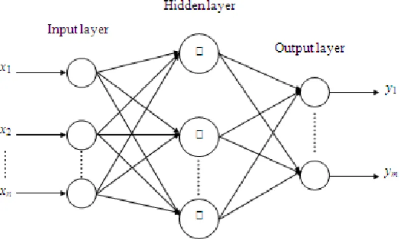
The RBFNN consists of three layers which include an input layer, a hidden layer, and an output layer arranged in a feedforward structure as can be seen in Fig. 1. The input layer receives n-dimensional input variables and submits them directly to the nodes in the hidden layer (Oh et al., 2012). The variables x1, x2, … xn
), (
) ( )
( ) ( ]
[ ] 1
[ i 1 i i 2 g i
i t wV t c rand P X c Rand P X
V
ki
i ij
j w x
y
1
) (
2
2
exp ) (
i i j j
i
c x x
where i = 1, 2, …, k, j = 1, 2, …, n, is the Euclidean norm, ci and
i are the center and the width of the ith Gaussian function in the hidden layer, respectively.Each node in the hidden layer is connected to the output nodes via modifiable weights. The output variables
y1, y2, …, ym from the nodes located at the output layer realize a linear combination of the activation levels of the
neurons positioned at the hidden layer. More specifically, the output of the jth output node can be expressed as:
where j = 1, 2, …, m and wij represents the modifiable connection weight between the ith hidden node and
the jth output node.
In this work, the RBFNN structure shown in Fig. 1 was trained by the adaptive CPSO to act as a feedback controller. In particular, the input layer receives three input variables namely, the error of the controlled plant (e), the error rate of change (Δe), and the summation of errors (∑e). In the hidden layer, seven nodes are used to represent seven radial basis functions utilizing the Gaussian kernel function of equation (1) above. Finally, in the output layer, there is only one output variable (u) which represents the controller output.
Fig. 1: Structure of the radial basis function neural network.
Particle Swarm Optimization:
As a population-based evolutionary technique, the PSO is a random-guided search optimization method which does not require derivative information from the problem being optimized. The PSO algorithm utilizes multiple candidate solutions for the optimized problem. These solutions are called particles and a group of these particles is called the swarm.
Collaborating simultaneously with each other, the particles in a swarm are allowed to fly in the search space of the problem seeking for the optimal position to land. In this journey, each particle adjusts its velocity and position according to its own experience and the experiences from other particles in the swarm. These experiences are gained by memorizing (recording) the best position reached by each particle and the best position reached by the entire swarm. Therefore, unlike other evolutionary algorithms like the GA, the PSO uses a memory in its operation to find the required solution of a given problem.
Standard PSO:
The standard PSO algorithm utilizes the local searching ability from the experience of each particle and the global searching ability from the experience of the entire swarm and combines these experiences together in an attempt to balance the exploration and the exploitation in finding the optimal solution.
As mentioned before, each particle has its own velocity and position which are updated in each iteration according to the following expressions (Liu et al., 2005):
(1)
(2)
] 1 [ ] [ ] 1
[t X t V t
Xi i i
, ,
, ,
) )(
(
max
min min min
max min
avg avg avg
f f w
f f f
f
f f w w w w
, 1 0
), 1
( 0
1
x x x
xn n n
In the above equations, Vi = [vi,1, vi,2, …, vi,n] and Xi = [xi,1, xi,2, …, xi,n] represent the velocity and position of
the ith particle, respectively. n is the number of decision variables in each particle, Pi represents the best previous
position reached by particle i (local-best solution), Pgis the best position among all particles in the swarm (global-best solution), rand(·) and Rand(·) are two random variables generated in the range [0,1], c1 and c2 are
two constants referred to as the acceleration coefficients which are used to control the maximum step size, and w
is the inertia weight whose task is to control the influence of previous velocity of a particle on its current velocity.
As can be observed from equation (3), the new velocity of a given particle is determined from its previous velocity, the distance between its current position and its previous best position, and the distance between its current position and the best position reached by the whole swarm. After adjusting its velocity, the particle is allowed to fly toward a new position using equation (4).
Adaptive Chaotic PSO:
As mentioned before, the standard PSO suffers from the premature convergence which leads the algorithm to fall into a local minimum in the search space. As a solution to this problem, several attempts have been made in (Liu et al., 2005; Song et al., 2007; Chuanwen and Bompard, 2005; Chuang et al., 2011) to handle this problem by incorporating the chaos optimization search into the standard PSO algorithm resulting in a more powerful CPSO optimization method. In this work, the adaptive CPSO version proposed in (Liu et al., 2005) is used to train the RBFNN controller. The details of this adaptive CPSO are described in the following.
Adaptive Inertia Weight:
In equation (3), the inertia weight (w) is used to balance the search between exploration and exploitation in PSO. Consequently, selecting a proper value for w is a crucial issue which affects the overall performance of the PSO. In order to get a good compromise between exploration and exploitation, the value of w is varied adaptively according to the value of the objective functions achieved by each particle. More specifically, the value of w is calculated according to the following:
where wmax and wmin represent the maximum and the minimum values of the inertia weight w, respectively, f
denotes the current objective function of the particle, fmin is the minimum objective function achieved by all the
particles, and favg is the average objective function of the current iteration.
The task of equation (5) is to alter the value of w adaptively according to the objective function so that particles with objective functions below average are moved with little steps while particles with objective functions above average are moved with large steps. This strategy in changing the value of w provides a good
balance between the local search and the global search of the CPSO algorithm (Liu et al., 2005).
Chaotic Local Search:
In order to enhance the searching ability and to avoid the premature convergence, chaotic dynamics along with the adaptive inertia weight described above are included in the PSO algorithm. In this context, the well-known logistic equation is utilized to provide the chaotic behavior. The logistic equation is defined by the following expression:
where µ is the control parameter, x is a variable, and n = 0, 1, 2, … .Despite the deterministic nature of equation (6), it exhibits chaotic dynamics when µ = 4 and x0{0,0.25,0.5,0.75,1}. In general, the above equation provides ergodicity, pseudo-randomness and irregularity which are necessary to boost the standard PSO performance (Liu et al., 2005).
(4)
(5)
, ..., , 2 , 1 ), 1 (
4 ( ) ( )
) 1
( cx cx i n
cx k
i k
i k
i
. ..., , 2 , 1 , min, max, min, ) ( )
( i n
x x x x cx i i i k i k
i
. ..., , 2 , 1 ),
( max, min,
) 1 ( min, ) 1
( x cx x x i n
x k i i
i i k
i
o T k p T k y k r MSE o
0 2 )] ( ) ( [In order to describe the chaotic local search process, equation (6) above can be re-written as:
where cxi is the ith chaotic variable, and k is the iteration number. The variable (k) i
cx
is distributed in the range (0,1) provided that the initial (0)(0,1)i
cx and that (0){0.25,0.5,0.75} i
cx . The following steps
clarify the chaotic local search algorithm:
Step 1: Set the iteration counter (k) to zero. Then, map the decision variables xi(k), i = 1, 2, …, n among the intervals (xmin,i, xmax,i), i = 1, 2, …, n to chaotic variables cxi(k)located in the interval (0,1) via the following
equation:
Step 2: Determine the chaotic variables
cx
i(k1)for the next iteration using equation (7).Step 3: Convert the chaotic variables
cx
i(k1)to decision variablesx
i(k1) using the following expression:Step 4: Evaluate the new solution with decision variables xi(k1), i = 1, 2, …, n. Step 5: If the new solution is better than [ (0),..., (0)]
1 ) 0 ( n x x
X or the predefined maximum number of iterations is reached, the new solution is the result of the chaotic local search; otherwise, let k = k + 1 and go back to Step 2.
Implementation of the Adaptive CPSO Technique to Train the RBFNN Controller:
By integrating the adaptive inertia weight and the chaotic local search described above into the standard PSO, a two-phased iterative strategy called adaptive CPSO is obtained. In this adaptive CPSO, the PSO with adaptive inertia weight is employed to achieve global exploration, while the chaotic local search is applied to achieve a local-oriented search (exploitation) (Liu et al., 2005).
The procedures of the adaptive CPSO proposed in this work to train the RBFNN controller are described in the following:
Step 1: Initialize the adaptive CPSO parameters: wmin, wmax, c1, c2, swarm size, and the maximum number of
iterations.
Step 2: Generate the initial swarm of N particlesrandomly within certain bounds, Xi = [xi,1, xi,2, …, xi,n],
where i = 1, 2, …, N, N is the number of particles,and n is the number of decision variables in each particle. In this swarm, each particle represents the entire modifiable parameters of a single RBFNN controller consisting of 25 decision variables. These decision variables include three input scaling factors, one output scaling factor, 14 variables representing the centers and widths of the radial basis functions in the hidden layer, and seven variables representing the weights between the hidden layer and the output layer.
In addition, initialize the initial particles’ velocities to zero. Since the problem in this work is to minimize the objective functions throughout the iterations, initialize Piand Pg to infinity, where Pi represents the best previous position reached by particle i (local-best solution) and Pgrepresents the best position among all particles in the swarm (global-best solution).
Step 3: Repeat until a stopping criterion is satisfied:
Step 4: Evaluate the objective function for each particle in the swarm (fi ; where i = 1, 2, …, N) using the mean square of error (MSE) criterion having the following form:
where r(k) and yp(k) are the reference signal (desired output) and the actual plant output at sample k, respectively, and To is the observation time (number of samples).
(7)
(8)
(9)
ij t ij j t ij ij t ij j t ij P x then X x If P x then X x If ] 1 [ min ] 1 [ ] 1 [ max ] 1 [ , , 1 0 )}, ( , min{ 1 0 )}, ( , max{ min max ) ( , max max min max ) ( , min min r x x r x x x r x x r x x x j j k j g j j j j k j g j j
Step 5: For each particle i, set Pi= Xi ; if fi < fbest[i], i N. Step 6: Find Pg such that
f
[
P
g]
f
i,
i
N
.
Step 7: Update the velocity of each particle, Vi[t+1], according to equations (3) and (5), then move each particle to its new position, Xi[t+1], using equation (4).
Step 8: Check the resulting position for each particle to ensure that the value of each member in the ith particle does not exceed the corresponding range assigned for that member by the following formula:
where max j
X and min
j
X represent the upper and the lower bounds, respectively, for member j in the ith
particle.
Step 9: Reserve the top N/5 particles.
Step 10: Implement the chaotic local search described before for the best particle, x k j n
j
g , 1,2,..., )
(
, and
g represents the index of the best particle. If the result of the chaotic local search is better than the original best particle, take this result as the best particle; otherwise take the original best particle.
Step 11: Decrease the search space according to the following expressions:
Step 12: Randomly generate 4N/5 new particles within the decreased search space.
Step 13: Construct the new population using the randomly generated 4N/5 new particles and the old top N/5 particles in which the best particle is replaced by the result of the chaotic local search.
Step 14: Stop if the maximum number of iterations is reached, and the particle with the best objective function is the final optimal RBFNN controller generated by the adaptive CPSO, otherwise, increase the iteration counter by one and go back to Step 3.
RESULTS AND DISCUSSION
This section is dedicated to assess the ability of the RBFNN controller trained by the adaptive CPSO to control nonlinear systems. In particular, the controller performance in terms of control accuracy and generalization ability is evaluated in controlling three different nonlinear systems.
The adaptive CPSO described before is employed to train the RBFNN controller. The parameters of the adaptive CPSO were set to the following values:
Swarm size (N): 60 particles, maximum number of iterations: 400, wmin: 0.2, wmax: 0.9, c1: 2, and c2: 2.
These values were found to be suitable for the current application after several simulation tests to control the following plants.
Plant 1:
This nonlinear plant is represented by the following difference equation (Shimal, 2001):
) ( ) 5 . 0 ) 1 ( )( 1 ( )) 8 . 0 ) 1 ( ( ) ( 8 . 0 ( ) 1
(k y k u k u k u k u k
y
Two different reference signals were used for this plant in order to test the generalization ability of the RBFNN controller. The first signal is a training signal to optimize the controller parameters, while the second one is a testing signal to evaluate how well the controller has been trained in the training phase. The training signal has the following definition:
(11)
(12)
200 161
5 . 0
161 121
3 . 0
121 81
4 . 0
81 41
6 . 0
41 0
2 . 0
) (
k k k k k
k rtrain
200 161
2 . 0
161 121
4 . 0
121 81
6 . 0
81 41
4 . 0
41 0
2 . 0
) (
k k k k k
k rtest
while the testing signal is defined by the following:
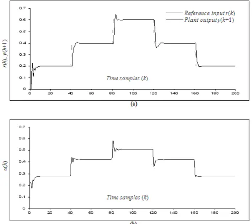
Fig. 2 shows the output response, the control signal, and the best MSE against iterations resulted from controlling Plant 1.
Despite the differences between the training and the testing signals, the RBFNN controller has done well in tracking the testing signal applied to Plant 1, as can be seen from Fig. 2 (a). This result indicates that this controller has good generalization ability. In terms of control accuracy, the RBFNN controller has achieved zero steady-state errors in all the parts of the testing signal with little oscillations at the start of each change in this signal.
Fig. 2 (b) depicts the control signal which shows the ability of the RBFNN controller to adapt its actions according to the variations in the testing signal. From Fig. 2 (c), it is obvious that the adaptive CPSO has achieved a fast convergence by minimizing the MSE to its near optimal value from the early stage of the optimization process.
(14)
/ 2 1 1
1 xu x(1 x )ex2
dt
dx
) 1
( ) 1 ( ) 1 (
2 /
2 1 2
2 2
x e
x x u x dt
dx x
M k
y k y
k y k y k
y
) 1 ( ) ( 1
) 1 ( ) ( 5 . 1 ) 1
( 2 2
Fig. 2: Plant 1 (a) output response (b) control signal (c) best MSE against iterations.
Plant 2:
Compared to Plant 1, this is a more complex nonlinear system which is described by the following difference equation (Al-Dulaimy, 2001):
where M0.5sin(0.5(y(k)y(k1))cos(0.5(y(k)y(k1))1.2u(k)
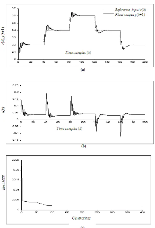
To evaluate the controller performance in controlling this plant, the same training and testing signals of equations (14) and (15) respectively, were used. Fig. (3) shows the output response, the control signal, and the best MSE against iterations resulted from controlling Plant 2.
Despite the complexity of Plant 2 resulted from the sine and cosine functions, Fig. 3 (a) shows that the RBFNN controller managed to control this complex nonlinear plant with some overshoots and oscillations at the start of each change in the testing signal. Keeping in mind the differences between the training and the testing signals, the controller has once again shown good generalization ability in controlling Plant 2. In order to cope with the difficulty of Plant 2, Fig. 3 (b) shows a more complicated control signal compared to the control signal resulted from controlling Plant 1 in Fig. 2 (b). This complex nature for the control signal was the result of adaptation made by the controller to handle the unexpected testing signal. As in Plant 1, Fig. 3 (c) indicates the fast convergence achieved by the adaptive CPSO to minimize the MSE from the first 100 iterations.
Plant 3:
Plant 3 is a bioreactor which represents a highly nonlinear chemical process. This process consists of a tank containing water, nutrients, and biological cells. Nutrients and biological cells are introduced into the tank and they are mixed in it. The dynamics of this process can be represented by the following nonlinear continuous time equations (Oysal et al., 2006):
The states of this process are given by the number of cells x1 and the amount of nutrients x2. The volume of
the tank content is maintained at a constant level by removing tank contents at a rate equal to the incoming flowrate, which is denoted by u. In the mathematical model of the bioreactor process, β= 0.02 is the growth rate parameter and γ= 0.48 is the nutrient inhibition parameter. The control objective in this process is to keep the amount of cells at a desired level. The initial conditions for the states of this process were taken as x1 = 0.1207
and x2 = 0.8801 (Oysal et al., 2006).
(16)
Fig. 3: Plant 2 (a) output response (b) control signal (c) best MSE against iterations.
In this control problem, it is desired to force the number of cells to follow the trajectory, )
15 / 15 cos( 0293 . 0 15 . 0 ) (
1 t t
x , and this signal was used as the training signal for the RBFNN controller. While as the testing signal, the trajectory,x1(t)0.150.0293cos(8t/15), was used to assess the generalization ability of the RBFNN controller. The fourth order Runge-Kuta method was utilized to numerically solve this continuous time model with a simulation step size of 0.1. Fig. 4 shows the output response, the control signal, and the best MSE against iterations for Plant 3.
achieved less steady-state error compared to the fuzzy controller used in (Oysal et al., 2006)to control the same process. Bearing in mind that the researchers in (Oysal et al., 2006) did not use a testing signal to evaluate the generalization ability of their controller. Fig. 4 (b) signifies the adaptation in the controller output to handle the testing signal. Similar to the previous plants, the adaptive CPSO has done well in terms of convergence speed, as it is evident from Fig. 4 (c).
A Comparative Study with a Neuro-Fuzzy Controller:
Both RBFNNs and neuro-fuzzy systems rely on similar concepts borrowed from artificial neural networks. However, RBFNNs are characterized by their simple structure compared to the structure of most neuro-fuzzy systems which require several hidden layers in their construction. In this regard, it is important to compare the performance of the RBFNN controller with that of a neuro-fuzzy controller, and this section is devoted for this comparison.
The neuro-fuzzy controller considered in this comparative study was proposed in (Pham and Xing, 1997). The structure of this controller consists of six layers whose tasks are to perform the fuzzy inference operations. In particular, Layer 1 has three nodes to receive the three input variables (e, Δe, and ∑e), which were described before for the RBFNN controller. Seven fuzzy sets are used for each of these input variables; as a result, there are 21 nodes in Layers 2 and 3. Layer 4 has 11 nodes which perform the max-product operator for fuzzy inferencing. To achieve the center of gravity defuzzification method, two nodes are included in Layer 5, and finally, one node is used in Layer 6 to produce the final controller output.
For a fair comparison, the same adaptive CPSO algorithm used to train the RBFNN controller was used to train the neuro-fuzzy controller with exactly the same parameter settings described before. In fact the only difference was in the number of decision variables. More precisely, 288 decision variables were required to represent each particle in the adaptive CPSO method for the neuro-fuzzy controller against only 25 decision variables for the RBFNN controller.
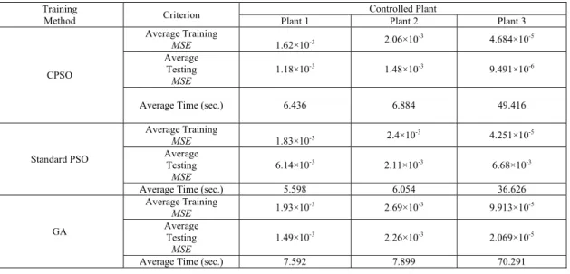
With the purpose of taking the stochastic nature of the adaptive CPSO into consideration and to achieve a reliable comparison study, 10 independent runs were conducted for each of the RBFNN controller and the neuro-fuzzy controller to control each plant. Then, the average training and testing MSE and the average time were taken as the basis in this comparative study. Table 1 summarizes the result of comparing the control performance of the two controllers in controlling the three plants considered before.
From Table 1, it is obvious that the RBFNN controller has taken less time in controlling the three plants compared to the neuro-fuzzy controller. This result highlights the main advantage of the RBFNN controller over the neuro-fuzzy controller which is the reduction in training time, an attribute required in real-time control applications.
In terms of control precision, Table 1 shows that the RBFNN controller has achieved less testing MSE for all the plants which indicates the superior generalization ability of the RBFNN controller compared to the neuro-fuzzy controller.
A Comparative Study with the Standard PSO and the GA:
In order to demonstrate the effectiveness of the adaptive CPSO in training the RBFNN controller, a comparative study was made with the standard PSO and the GA to train the RBFNN controller. In this comparison, the same plants with the same training and testing signals described before were used. For the three optimization methods, 25 decision variables were needed to represent the RBFNN controller.
The parameter values of the adaptive CPSO were described at the beginning of the result and discussion section, while the parameters of the standard PSO was set to the following values; swarm size (N): 60 particles, maximum number of iterations: 400, w: 0.7, c1: 2, and c2: 2, and finally, the parameters of the GA were given
the following values; population size: 60, maximum number of generations: 400, crossover probability (Pc): 0.85, and mutation probability (Pm): 0.1.
In order to eliminate stochastic discrepancy, 10 independent runs were made for each optimization method. Table 2 gives the comparison results.
In terms of control accuracy, the superiority of the adaptive CPSO over the standard PSO and the GA can be easily seen from Table 2. Particularly, the adaptive CPSO has achieved less training and testing MSE for all the plants (except the average training MSE for plant 3) compared to the other optimization methods. In terms of training time, Table 2 reveals that there is no significant difference among the three optimization methods except for Plant 3, where the GA has taken the longest time.
Conclusions:
An adaptive CPSO technique was utilized to train a RBFNN to act as a controller for nonlinear dynamical systems. In this control strategy, there is no need for a teaching signal to train the RBFNN controller. The adaptive CPSO was applied to optimize all the modifiable parameters of the RBFNN, namely the centers and widths of the radial basis functions along with the connection weights between the hidden layer and the output layer of the RBFNN.
hand, the RBFNN controller has achieved a more precise control performance with better generalization ability compared to the neuro-fuzzy controller. Moreover, from a comparative study, it was evident that the adaptive CPSO outperforms the standard PSO and the GA in training the RBFNN controller, where the adaptive CPSO has achieved the least training and testing MSE.
Table 1: Results of comparing the RBFNN controller with the neuro-fuzzy controller (both are trained by the adaptive CPSO technique)
Controlled Plant
Neuro-Fuzzy Controller
RBFNN Controller
Average Training
MSE
Average Testing
MSE
Average Time (sec.)
Average Training
MSE
Average Testing
MSE
Average Time (sec.) Plant 1
1.53×10 2.45×10⁻³ 38.730-3 1.62×10⁻³ 1.18×10⁻³ 6.436
Plant 2
1.64×10 24.61×10⁻³ 40.657-3 2.06×10 1.48×10⁻³ 6.884-3
Plant 3
4.194×10 2.484×10⁻⁵ 183.342-5 4.684×10 9.491×10⁻⁵ 49.416-6
Table 2: Results of comparing the performance of the adaptive CPSO, the standard PSO, and the GA as the training methods for the RBFNN controller
Training
Method Criterion
Controlled Plant Plant 1
Plant Plant 2 3
CPSO
Average Training
MSE 1.62×10⁻³ 4.684×102.06×10-3 -5
Average Testing
MSE
1.18×10⁻³
1.48×10 9.491×10⁻³ -6
Average Time (sec.) 6.436 6.884 49.416
Standard PSO
Average Training
MSE 1.83×10⁻³ 2.4×10⁻³ 4.251×10⁻⁵
Average Testing
MSE
6.14×10⁻³ 2.11×10⁻³ 6.68×10⁻³
Average Time (sec.)
5.598 36.6266.054
GA
Average Training
MSE 1.93×10⁻³ 2.69×10 9.913×10⁻³ -5
Average Testing
MSE
1.49×10⁻³ 2.26×10 2.069×10⁻³ -5
Average Time (sec.)
7.592 70.2917.899
REFERENCES
Al-Dulaimy, A.I., 2001. Evolving neuro-controllers for nonlinear dynamical systems, M.Sc. Thesis, University of Technology, Baghdad-Iraq.
Chen, J.Y., Z. Qin and J. Jia, 2008. A PSO-Based Subtractive Clustering Technique for Designing RBF Neural Networks. IEEE Congress on Evolutionary Computation, Hong Kong-China, pp: 2047-2052.
Chen, Z. and P. Qian, 2009. Application of PSO-RBF Neural Network in Network Intrusion Detection. Third International Symposium on Intelligent Information Technology Application, Nanchang-China, pp: 362-364.
Chuang, L.-Y., C.-J. Hsiao and C.-H. Yang, 2011. Chaotic Particle Swarm Optimization for Data Clustering. Expert Systems with Applications, 38(12): 14555-14563.
Chuanwen, J., and E. Bompard, 2005. A Self-Adaptive Chaotic Particle Swarm Algorithm for Short Term Hydroelectric System Scheduling in Deregulated Environment. Energy Conversion and Management, 46(17): 2689-2696.
Dehuri, S., R. Roy, S.-B. Cho and A. Ghosh, 2012. An Improved Swarm Optimized Functional Link Artificial Neural Network (ISO-FLANN) for Classification. The Journal of Systems and Software, 85(6): 1333-1345.
Dong, X., C. Wang and Z. Zhang, 2010. RBF Neural Network Control System Optimized by Particle Swarm Optimization. 3rd IEEE International Conference on Computer Science and Information Technology, Chengdu-China, pp: 348-351.
Jihong, Q., Z. Juan and C. Nanxiang, 2010. Groundwater Table Prediction Based on Improved PSO Algorithm and RBF Neural Network. International Conference on Artificial Intelligence and Computational Intelligence, Sanya-China, pp: 228-232.
Li-kun, Z. and L. Hong-zhao, 2011. Operating Parameter Optimization of Centrifuge Based on APSO-RBF. International Conference on Transportation, Mechanical, and Electrical Engineering, Changchun-China, pp: 2111-2114.
Lin, F.-J., L.-T. Teng and M.-H. Yu, 2008. Radial Basis Function Network Control with Improved Particle Swarm Optimization for Induction Generator System. IEEE Transactions on Power Electronics, 23(4): 2157-2169.
Liu, B., L. Wang, Y.-H. Jin, F. Tang and D.-X. Huang, 2005. Improved Particle Swarm Optimization Combined with Chaos. Chaos, Solitons and Fractals, 25(5): 1261-1271.
Liu, W., Y. Duan, K. Shao and K. Wang, 2007. Chaotic Synchronization of Adaptive Inverse Control Based on Hybrid Particle Swarm Optimization Algorithm. IEEE International Conference on Mechatronics and Automation, Harbin-China, pp: 2409-2413.
Liu, J., C. Wu, X. Wang, W. Wang and T. Zhang, 2010. A Hybrid Control for Elevator Group System. Third International Workshop on Advanced Computational Intelligence, Jiangsu-China, pp: 491-495.
Liu, J., C. Wu, M. Liu, E. Gao and G. Fu, 2011. RBF Optimization Control Based on PSO for Elevator Group System. International Conference on Information Science and Technology, Jiangsu-China, pp: 363-368.
Man, C.-T., K. Wang and L.-Y. Zhang, 2009. A New Training Algorithm for RBF Neural Network Based on PSO and Simulation Study. 2009 World Congress on Computer Science and Information Engineering, Los Angeles -USA, pp: 641-645.
Oh, S.-K., W.-D. Kim, W. Pedrycz and S.-C. Joo, 2012. Design of K-Means Clustering-Based Polynomial Radial Basis Function Neural Networks (pRBF NNs) Realized with the Aid of Particle Swarm Optimization and Differential Evolution. Neurocomputing, 78(1): 121-132.
Oysal, Y., Y. Becerikli and A.F. Konar, 2006. Modified Descend Curvature Based Fixed Form Fuzzy Optimal Control of Nonlinear Dynamical Systems. Computers and Chemical Engineering, 30(5): 878–888.
Pham, D. T. and L. Xing, 1997. Neural Networks for Identification, Prediction and Control. Springer-Verlag, 3rd Printing, London.
Qasem, S.N., S.M. Shamsuddin and A.M. Zain, 2012. Multi-Objective Hybrid Evolutionary Algorithms for Radial Basis Function Neural Network Design. Knowledge-Based Systems, 27: 475-497.
Shimal, A.F., 2001. CMAC as an adaptive controller of nonlinear systems. M.Sc. Thesis, University of Technology, Baghdad-Iraq.
Song, Y., Z. Chen and Z. Yuan, 2007. New Chaotic PSO-Based Neural Network Predictive Control for Nonlinear Process. IEEE Transactions on Neural Networks, 18(2): 595-600.
Šušić, M., A. Ćosić, A. Ribić and D. Katić, 2011. An Approach for Intelligent Mobile Robot Motion Planning and Trajectory Tracking in Structured Static Environments. IEEE 9th International Symposium on
Intelligent Systems and Informatics, Subotica-Serbia, pp: 17-22.
Tan, Q.Y. and Y. Song, 2008. Sidelobe Suppression Algorithm for Chaotic FM Signal Based on Neural Network. 9th International Conference on Signal Processing, Beijing-China, pp: 2429-2433.
Wang, P., L. Xie and Y. Sun, 2009. Application of PSO Algorithm and RBF Neural Network in Electrical Impedance Tomography. The 9th International Conference on Electronic Measurement & Instruments,
Beijing-Chian, pp: 2-517 to 2-521.
Wang, S., D. Lv, Z. Li and H. Li, 2011. A Novel RBF-PID Control Strategy for Turbine Governing System Based on Chaotic PSO. Proceedings of the 8th World Congress on Intelligent Control and Automation,


![N Acetyl N {2 [(Z) 2 chloro 3,3,3 trifluoroprop 1 enyl]phenyl}acetamide](data:image/gif;base64,R0lGODlhAQABAIAAAP///wAAACH5BAEAAAAALAAAAAABAAEAAAICRAEAOw==)