27
Designing a green location routing inventory problem considering
transportation risks and time window: a case study
Neda Manavizadeh
1*, Mahnaz Shaabani
1, Soroush Aghamohammadi-Bosjin
21Department of Industrial Engineering, Khatam University, Tehran, Iran
2 School of Industrial Engineering, College of Engineering, University of Tehran, Tehran, Iran [email protected], [email protected], [email protected]
Abstract
This study introduces a green location, routing and inventory problem with customer satisfaction, backup distribution centers and risk of routes in the form of a non-linear mixed integer programming model. In this regard, time window is considered to increase the customer satisfaction of the model and transportation risks is taken into account for the reliability of the system. In addition, different factors are detected as the major factors affecting the risk of routs and a fuzzy TOPSIS method is applied to rank the related risk factors. Next, due to the complexity of the investigated model, two algorithms including multi-objective gray wolf optimization algorithms (MOGWO) and Non-Dominated Sorting Genetic algorithm (NSGA-II) are applied to solve the large-sized instances. The results prove the superiority of MOGWO in dealing with large-sized instances. In the next step, some sensitivity analysis is implemented on the model based on a case study and the related results of case study are reported as well.
Keyword: Location routing inventory, green supply chain, backup strategy, customer satisfaction, fuzzyTOPSIS, multi objective gray wolf optimization algorithm.
1- Introduction
Today, the role of transportation is critical in economic development of supply chains by facilitating the availability of products for the long-distance factories. Delivering process in a supply chain (SC), incorporates shipment of raw materials from suppliers to production centers (PCs) and transformation of semi-finished products between the PCs and customers. Due to the multiplicity of transportation activities, shipping costs include high percentage of logistic costs. Therefore, managing the related costs of transportation has become a major issue for the supply chain decision makers. In this regard, there is a competitive market between supply chains (SCs) to reduce their costs and enhance their profit. Many researches have considered strategic and tactical decisions in SC problems including location, routing and inventory decisions to develop integrated SCs (Zheng et al. 2019; Rabbani et al, 2017; Malladi and Sowlati 2017). Integration of these decisions is one of the most important factors that significantly reduce the cost of the chain and lead to increase of customer satisfaction. Inaccurate location of facilities and inappropriate route selection lead to high transportation costs.
*Corresponding author
ISSN: 1735-8272, Copyright c 2020 JISE. All rights reserved
Journal of Industrial and Systems Engineering Vol. 12, No. 4, pp. 27 - 56
28
Moreover, inappropriate transportation system leads to higher amount of carbon emissions. Supply chain management (SCM) includes purchasing management, inventory control, production and distribution.
Green Supply Chain Management (GSCM) joints economic aspects of SC with environmental aspects in order to manage the environmental effects of the system besides the maximization the performance of the entire SC (Abu seman et al, 2019). The public awareness of climate change and the growing concern about the environmental conditions has made GSCM an important issue in the production and distribution cycle (Fang and azhang, 2018). This study presents a new location-routing-inventory problem by taking into consideration the environmental aspects, backup strategies, time window and transportation risks to enhance the customer satisfaction and reliability of the system simultaneously.
Clearly, strategic decisions of a SC affect the tactical decisions of the SC including inventory and routing decisions. As a result, a location- inventory-routing model covers the strategic and tactical decisions of a SC. However, combination of these issues increases the complexities of the main problem (Diabat et al, 2015). Many of developed models in the SCN consider these important decisions separately while they are dependent by nature. This study introduces a new multi objective model integrating location, routing and inventory problem issues as a joint location- routing-inventory problem (LRIP). This model considers backup distribution centers in order to decrease the shortage and time window to increase the customer satisfaction. In addition, this paper takes into account different factors affecting the stability of routs to select the best rout with the least level of risk for shipment of products. In this regard, the main contributions of this study are stated as follows:
Developing a new multi-objective location- inventory-routing problem. Considering backup centers to decrease the shortage and satisfy the customers.
Considering a hard time window for delivery process to enhance the customer satisfaction. Considering the transportation risks in model to enhance the reliability of the system. Applying a fuzzy TOPSIS method for analyzing the factors affecting the reliability of routes. Applying a multi-objective gray wolf optimization algorithm to efficiency solve the problem. The remainder of this article is arranged as follows: Section 2 reviews relevant related literature. The uncertain green location- routing inventory model is proposed in section 3. The NSGA-II and MOGWO algorithms are presented in section 4. Model validation, numerical results and sensitivity analysis are reported in section 5. Comparative result from before section discuss in section 6. Sensitivity analysis is given in section 7. At last, in section 8, conclusions and future suggestions are stated.
2-Literature review
This section discusses about different studies related to location-routing-inventory problem, Green LRIP and LRIP with risk.
2-1- Location-routing-inventory problem
For the first time, Liu and Lee (2003) presented a LRIP in which they assumed heterogeneous fleet and unlimited capacity for depots. They solved model using a two-phase heuristic algorithm. Liu and Lee (2005) developed their model by using Tabu Search (TS) and Simulated Annealing (SA) algorithms to solve their model. They didn't consider shortage and ordering cost in their model. Zhang, Zujun and Jiang (2008) developed a multi-period single-item LRIP with a homogeneous fleet and uncertain demand and solved their model by a genetic algorithm. Sajjadi and Cheraghi. (2011) studied a multi- commodity, three-echelon and single-period SC with stochastic demand. In their model, warehouses had limited capacity and 3PL companies provided space in order to storage items in DCs. Seyyed Hosseini, Bozorgi-Amiri and Daraei. (2014) introduced a single-objective model for inventory, routing and location decisions. They considered stochastic demand, shortage and random disruption at distribution centers (DCs) and applied a metaheuristic algorithm to solve the proposed model. Dehghani, Behfar and Jabalameli. (2016) developed a mathematical model for LRIP and used SA algorithm for solving the problem. In their model, the demands of retailers were ucertain. Amiri aref, Klibi and Zied Babai. (2017)
29
presented a multi-source, multi-period, multi-echelon SC LRIP with uncertain demand. In their model, they examined the impact of shipping costs, inventory holding costs, and product referrals. They used a Sample Approximation method to solve the proposed model.
Yuchi et al. (2018) studied a LRIP in a closed-loop supply chain in which the remanufacturing centers were located. For solving their model, they used hybrid method TS and SA algorithms. Rabbani et al. (2018) formulated a multi-objective stochastic model for a locating-routing problem by considering inventory control and the risk of wastes for humans. They integrated a NSGA-II and the Monte Carlo simulation to solve the model. Momeni Kia et al. (2018) designed a two-objective model for LRIP with soft time windows. They applied three metaheuristics including MOPSO, PESA_II and NSGA-II algorithms to solve the model. Guo et al. (2018) examined the LRIP in a close loop SC and proposed a non-linear integer programming model with the aim of reducing system costs including inventory, routing and transportation costs. They used a hybrid metaheuristic comprised of SA and GA algorithms to solve the model. Zheng, Yin and zhang. (2019), formulated a nonlinear LRIP that minimized the total system costs including the inventory, shipping and opening costs of the DCs. They used exact algorithm based on the Generalized Benders Decomposition (GBD) to solve the model.
2-2- Green LRIP
In the most of researches in literature, routing (LR), inventory-routing (IR) and location-inventory (LI) problems have included environmental aspects in their model. Treital, Nolz and Jammerneg.(2012) proposed an IR problem with environmental aspects and applied a case study for their model. They didn’t consider inventory costs in their model. In their model, emission was related to vehicle type and travelling distance. Soysal et al (2015) addressed an IRP for perishable products with environmental aspects. they assumed demand is uncertain. The environmental impacts of their model were related to reducing CO2 emission, fuel consumption and food waste. In addition, Soysal et al (2017) proposed a green IR problem by regarding Co2 emission, total system costs and perishable goods simultaneously with uncertain demand. They applied a case study with two suppliers and showed the reduced rate of Co2 emission is about 8-33%. Niakan and Rahimi (2015) presented an IRP in field the of medication distribution. They assumed that demand, transportation cost, and shortage cost were fuzzy parameters. Also, they showed that greenhouse gas (GHG) emission was related to transportation system. Rahimi, Babol and Rekik. (2017) developed an inventory routing problem with green considerations. Their model had three objectives and included profit of the system, service level and environmental effects of distribution operations. To solve the model, they used the NSGA-II algorithm. Rau, Budimana and Widyadanab. (2018) proposed a multi-objective IRP with environmental aspects. In their model, the Co2 emission comes from the fuel consumption of vehicles. They proposed a discrete multi-objective particle swarm optimization (PSO) to solve the model. They showed their model reduced the total cost between 17% - 22% and total emission between 19%-22%. Guido, Michelia and Fabio Mantella. (2018) offered an inventory routing problem with uncertainty demand that simultaneously considered emissions GHG and heterogeneous fleets. In order to reduce concerns about air pollution, they consider four carbon control strategies. Dukkanci et al. (2019) addressed a green LRIP and considered the speed and weight of vehicles as the major factors affecting the fuel consumption of vehicles.
As the literature review shows, there are a few researches considering environmental aspects in LRIPs. In this regard, the green LRIPs can be divided into two categories: The LRIPs with electric vehicle (EV) that focus on green VRP and developed electric vehicle problem (EVRP). The second group decreases the emissions by paying attention the distance traveled by vehicles (Zhang et al., 2018). According to the previous section there are some gaps in the context of LRIP as follows:
Considering the reliability of transportation system in a LRIP problem.
Analyzing the factors affecting the risk of routs for the delivery of items in a LRIP. Considering hard time windows for the shipment of products in a LRIP problem. Considering environmental factors in a multi-objective LRIP problem.
30
Applying a new multi objective metaheuristic problem for a LRIP.
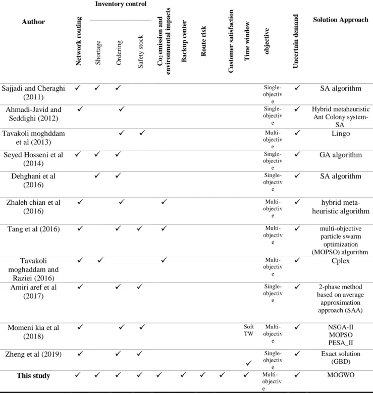
Table 1 shows the summary of literature review section and highlights the research gaps.
Table 1. Summation of the literature about LRIPs.
Solution Approach U n ce rt ai n d em an d ob je ct ive T im e w in d ow C u st o m er s a ti sf a ct ion R ou te r is k B ac k u p c en te r em is si on an d 2 Co en vi ron m en ta l im p ac ts Inventory control N et w or k r ou ti n g Author S af et y s toc k O rde ri n g S hor ta g e SA algorithm Single- objectiv e Sajjadi and Cheraghi
(2011)
Hybrid metaheuristic Ant Colony system-
SA Single- objectiv e Ahmadi-Javid and Seddighi (2012) Lingo Multi-objectiv e Tavakoli moghddam
et al (2013)
GA algorithm Single- objectiv e Seyed Hosseni et al
(2014) SA algorithm Single- objectiv e Dehghani et al
(2016) hybrid meta-heuristic algorithm Multi-objectiv e Zhaleh chian et al
(2016) multi-objective particle swarm optimization (MOPSO) algorithm Multi-objectiv e
Tang et al (2016)
Cplex Multi-objectiv e Tavakoli moghaddam and Raziei (2016) 2-phase method based on average
approximation approach (SAA) Single- objectiv e
Amiri aref et al (2017) NSGA-II MOPSO PESA_II Multi-objectiv e Soft TW
Momeni kia et al (2018) Exact solution (GBD) Single- objectiv e
Zheng et al (2019)
MOGWO Multi-objectiv e This study
31
3-Problem description
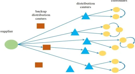
In this model a three-level SC consisted of suppliers, distribution/backup centers and customers, is designed. The products are transferred directly from the suppliers to the distribution and backup centers. The model aims to minimize the total cost, risk of routes and CO2 emission, while selecting and locating a set of DCs, allocating customers to DCs and timing the shipments of vehicles to fulfill the customer demand. The main assumptions of the model are as follows:
3-1- Assumptions
Inventory review of DCs is continuous. When inventory level of distribution center 𝐾′reaches its reorder point 𝑅𝑂𝑃𝑘′. 𝑄𝑘′ units are ordered
Each retailer is visited by only one vehicle.
Transportation fleet is heterogeneous and vehicles capacities are not equal. Each retailer is served by only one DC.
Time window is hard. In other word, customer demand must be met within a specific time interval. After serving customer demand allocated to a DC, the vehicle returns back to the DC.
Customer demand is uncertain and follows normal distribution.
Network risk parameter is a combination of factors including road security, weather conditions and traffic which are considered as triangular fuzzy numbers.
Figure 1 illustrates the overview of the supply chain network.
Fig 1. The supply chain network examined
3-2- Fuzzy TOPSIS
According to assumption, the risk of transportation system increases by traffic, situation of roads and weather conditions. It should be note that each of mentioned risk factors have different degree of importance. Converting these factors to a single factor is applied utilizing fuzzy TOPSIS (refer to Abbasi Parizi et al (2018) for more details). Assume that 𝑟 and 𝑙 indicate alternatives and decision factors, respectively. The Risk of rout (𝛼𝐼𝐼′𝑣2) is calculated based on the instruction stated as follows:
1- Determining effective factors on risk of the route (like traffic, weather conditions, and situations of the roads) and weighting them,
32
3- Computing risk of each route using sum of weights allocated to route risk factors. 4- Composing a matrix for risk of the routes from node i to node j.
5- Selecting the route with the lowest risk.
The proposed fuzzy TOPSIS approach is defined as follows:
The Fuzzy factors must be defined before the optimization of the model, so they are calculated according to the related various features. For the first time, Yoon and Hwang in 1981 developed The TOPSIS method. TOPSIS is a multi-criterion decision-making (MCDM) method for ranking a number of alternatives with respect to their various criteria. The fuzzy TOPSIS is applicable when the weight of proposed criteria is unknown. In this regard, the closest Fuzzy Positive Ideal Solution (FPIS) and the farthest Fuzzy Negative Ideal Solution (FNIS) are selected as the factor range. According to (abbasi- parizi, 2018), the procedure of fuzzy TOPSIS can be expressed in following steps:
Definition 1: It is assumed that 𝑎̃ = (𝑎1. 𝑎2. 𝑎3) is a triangular fuzzy number (TFN). The membership function of 𝑎̃ described the following relation:
𝑡𝑟𝑛(𝑥: 𝑎1. 𝑎2. 𝑎3) =
{
0 𝑐 𝑥 − 𝑎1
𝑎2− 𝑎 1
𝑎1< 𝑥 ≤ 𝑎2
𝑎3− 𝑥
𝑎3− 𝑎2
𝑎2 < 𝑥 ≤ 𝑎3
0 𝑥 > 𝑎3
(1)
Definition 2: If the 𝑎̃ = (𝑎1. 𝑎2. 𝑎3) and 𝑏̃ = (𝑏1. 𝑏2. 𝑏3) are two fuzzy number, then the distance between 𝑎̃. 𝑏̃ is calculated as:
𝑑(𝑎̃. 𝑏̃) = (|𝑏1− 𝑎3|, |𝑏2− 𝑎2|, |𝑏3− 𝑎1|) (2)
Step1:D denotes a fuzzy decision matrix as follows:
𝐷 = [
𝑥̃11 𝑥̃12 … 𝑥̃1𝑛
𝑥̃21
⋮
𝑥̃22 …
⋮ ⋯ ⋱ 𝑥̃2𝑛
⋮ 𝑥̃𝑚1 𝑥̃𝑚2 … 𝑥̃𝑚𝑛
] and 𝑥̃𝑟𝑙 = (𝑎𝑟𝑙. 𝑏𝑟𝑙. 𝑐𝑟𝑙) (3)
Step2: The fuzzy decision matrix is normalized as follows:
𝑅̃ = [𝑟̃𝑟𝑙]𝑀×𝑁 (4)
𝑟𝑟𝑙 = (𝑎𝑟𝑙 𝑐 𝑟𝑙∗
⁄ .𝑏𝑟𝑙
𝑐𝑖𝑗∗
⁄ .𝑐𝑟𝑙
𝑐𝑟𝑙∗
⁄ ) . 𝑐𝑟𝑙∗ = max 𝑐𝑟𝑙 benefit criteria (5)
𝑟𝑟𝑙 = (𝑎𝑟𝑙 −
𝑐𝑟𝑙
⁄ .𝑎𝑟𝑙−
𝑏𝑟𝑙
⁄ .𝑎𝑟𝑙−
𝑎𝑟𝑙
⁄ ) . 𝑎𝑟𝑙− = min 𝑎
𝑟𝑙 cost criteria (6)
Step3: The weighted normalized decision matrix is calculated. 𝑤̃𝑟𝑙 is the weight factor of fuzzy parameters as follows:
33
𝑉 = [
𝑣̃11 𝑣̃12 … 𝑣̃1𝑛
𝑣̃21
⋮
𝑣̃22
⋮ … ⋱ 𝑣̃2𝑛⋮ 𝑣̃𝑚1 𝑣̃𝑚2 … 𝑣̃𝑚𝑛
] = [
𝑤̃11𝑟̃11 𝑤̃12𝑟̃12 … 𝑤̃1𝑛𝑟̃1𝑛
𝑤̃21𝑟̃21
⋮
𝑤̃22𝑟̃22
⋮ …
⋱ 𝑤̃2𝑛⋮𝑟̃2𝑛 𝑤̃𝑚1𝑟̃𝑚1 𝑤̃𝑚2𝑟̃𝑚2 … 𝑤̃𝑚𝑛𝑟̃𝑚𝑛
] (8)
Step4: The fuzzy ideal (positive) and fuzzy negative-ideal solutions are determined as follows.
𝐴∗= (𝑣̃1∗. 𝑣̃2∗. 𝑣̃3∗) = {(𝑚𝑎𝑥𝑣𝑟𝑙|𝑟 = 1.2. ⋯ . 𝑚). 𝑙 = 1.2. ⋯ . 𝑛} (9)
𝐴−= (𝑣̃1−. 𝑣̃2−. 𝑣̃3−) = {(𝑚𝑖𝑛𝑣𝑟𝑙|𝑟 = 1.2. ⋯ . 𝑚). 𝑙 = 1.2. ⋯ . 𝑛} (10)
Step5: The total fuzzy distance between each component, the positive and negative ideal solutions are calculated as follows:
(11)
𝑑̃𝑟∗ = ∑ 𝑑(𝑣̃𝑟𝑙. 𝑣̃𝑙∗) 𝑛
𝑙=1
𝑟 = 1.2. … . 𝑚
(12)
𝑑̃𝑟−= ∑ 𝑑(𝑣̃𝑟𝑙. 𝑣̃𝑙−) 𝑛
𝑙=1
𝑟 = 1.2. … . 𝑚
Step 6: Convert the similarity index to the Ideal Solution as follows:
𝐶̃𝑟∗=
𝑑̃𝑟 −
𝑑̃𝑟 −+ 𝑑̃ 𝑟
∗ 𝑟 = 1.2. … . 𝑚
(13) It is obvious that fuzzy parameters are obtained as 𝑎̃ = (𝑎1. 𝑎2. 𝑎3). For example, for the risk factor;
𝛼̃𝐼𝐼′𝑣 = (𝛼1𝐼𝐼′𝑣. 𝛼2𝐼𝐼′𝑣. 𝛼3𝐼𝐼′𝑣); the relative closeness to the Ideal Solution is calculated as follow as:
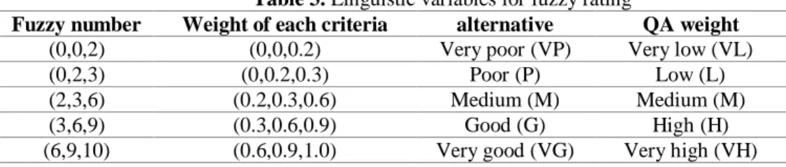
Table 3. Linguistic variables for fuzzy rating
Fuzzy number Weight of each criteria alternative QA weight
(0,0,2) (0,0,0.2) Very poor (VP) Very low (VL)
(0,2,3) (0,0.2,0.3) Poor (P) Low (L)
(2,3,6) (0.2,0.3,0.6) Medium (M) Medium (M)
(3,6,9) (0.3,0.6,0.9) Good (G) High (H)
(6,9,10) (0.6,0.9,1.0) Very good (VG) Very high (VH)
Table 3 shows the importance weight risk factors and the related rating of qualitative criteria. In the next step, the results of each factor are achieved using the decision maker's opinions. The related results are reported in table 4.
Table 4. fuzzy decision and weight matrix
alternative 𝑪𝟏 𝑪𝟐 𝑪𝟑
𝑨𝟏 (3,6,10) (5,8,10) (7,9,10)
𝑨𝟐 (2,5.7,10) (0,6,9) (5,8.4,10)
𝑨𝟑 (4,7,10) (7,9,10) (5,9,10)
weight (0.65,0.82,1) (0.5,0.71,0.93) (0.5,0.74,1)
According to relations (5)- (9), the fuzzy weighted normalized decision matrix described in table 5.
Table 5. The results of the fuzzy weighted normalized decision matrix
alternative 𝑪𝟏 𝑪𝟐 𝑪𝟑
𝑨𝟏 (0.42, 0.69,1) (0.5,0.8,1) (0.65,0.55,0.71)
𝑨𝟐 (0.35,0.77,1) (0,0.6,0.9) (0.5,0.6,1)
34 Then the FPIS and FNIS are determined:
𝐴∗= {(1.1.1). (1.1.1). (0 ∙ 5.0 ∙ 5.0 ∙ 5)} 𝐴−= {(0 ∙ 3.0 ∙ 3.0 ∙ 3). (0.0.0). (1.1.1)}
Finally, the distance between each component, the positive and negative ideal solutions are reached and the closest factor to ideal solution is reported in table 6.
Table 6: fuzzy distance and closeness coefficient
A* A-
𝑪̃𝒓∗
d(A1,) 2.57 2.78 0.517
d(A2,) 1.84 2.34 0.559
d(A3,) 2.18 1.95 0.472
Based on the above mentioned, the merged risk is calculated and will be used in the model.
3-3- Mathematical model
Symbols Definition
Index sets
𝑘′ Set of potential DCs
𝑘 Set of backup DCs
𝑖 Set of customers (or retailers)
𝐼 = {𝑘′∪ 𝑖} Set of customers and DCs
𝑣𝑖 Set of available vehicles from supplier O to DC k
𝑣2 Set of available vehicles from DCk to retailers and between them
𝑉 = 𝑣1∪ 𝑣2 Set of vehicles
𝑂 supplier
parameters
𝑓𝑓𝑘′ establishing cost of candidate 𝐷𝐶𝑘′
𝑓𝑘 establishing cost of candidate backup 𝐷𝐶𝑘
𝜇𝑖 mean yearly demand of retailer i
𝜎𝑖2 yearly demand variance at retailer i
𝐷𝑖 demand of retailer i
𝑓𝑘′ pollution cost of candidate backup 𝐷𝐶𝑘
ℎ𝑘′ inventory holding cost per unit of product at 𝐷𝐶𝑘′
𝑐𝑜𝑘′′ fixed administrative cost of ordering to supplier O by 𝐷𝐶𝑘′
𝑠𝑎𝑓𝑒𝑡𝑦 𝑘 holding cost of safety stock at backup 𝐷𝐶𝑘
𝑡𝑟𝑜𝑘𝑣1 transportation cost from supplier O to backup center 𝐷𝐶𝑘by vehicl𝑣1e
𝑚𝑜𝑘𝑘′ fixed cost of transportation from backup center 𝐷𝐶𝑘to 𝐷𝐶𝑘′
𝑐𝑜𝑠𝑡𝑜𝑘′𝑣1 Shipment cost per unit from supplier O to 𝐷𝐶𝑘′ by vehicle 𝑣1
𝛾𝑣 pollution cost of vehicle 𝑣
𝜌𝑣 amount of fuel consumption of vehicle 𝑣 while loaded full
𝜌𝑜𝑣 amount of fuel consumption of vehicle 𝑣 while unloaded
𝑑1𝑜𝑘′ distance between 𝐷𝐶𝑘′ and supplier O
𝑑2𝑜𝑘 distance between backup center 𝐷𝐶𝑘 and supplier O
𝑑3𝑖𝑗 distance between nodes iand j
𝑑𝑘𝑘′′ distance between backup center 𝐷𝐶𝑘 and 𝐷𝐶𝑘′
𝑐𝐼𝐼′ transfer cost of product from DCs to retailers i and between them
𝑐𝑎𝑝1𝑣1 capacity of vehicles 𝑣1
𝑐𝑎𝑝2𝑘′ capacity of 𝐷𝐶𝑘′
𝑐𝑎𝑝3𝑣2 capacity of vehicles 𝑣2
𝑐𝑜𝑠𝑡𝑘′′ shortage cost a𝑡 𝐷𝐶𝑘′
35
𝑈 A big number
𝑡̃𝐼𝐼′𝑣2 time needed to travelling from node 𝐼 to node 𝐼′ by vehicle 𝑣2
𝑠𝑡̃𝐼′ time needed to serve node𝐼′
𝑒̃𝐼′ earliest start time to serve node 𝐼′
𝑙̃𝐼′ latest start time to serve node𝐼′
𝐿′ upper level of inventory
𝑧𝛼 confidence level for inventory
𝑙𝑡̃𝑘′ lead time of 𝐷𝐶𝑘′
𝛼̃𝐼𝐼′𝑣2 Route risk of driving from node 𝐼 to node 𝐼′ using vehicle 𝑣2
Decision variables:
𝑥𝑘𝑘′= {1
0 In case of shortage at 𝐷𝐶𝑘
′, if products are transferred from backup center 𝐷𝐶𝑘 otherwise
𝑥𝑘′ = {10 if backup center 𝐷𝐶𝑘 selected
otherwise
𝑠𝑘′′ = {10 If distribution center 𝐷𝐶𝑘′ is opened
otherwise
𝑄𝑜𝑘′ ′𝑣1= {1
0 If order from supplier O for
𝐷𝐶𝑘′is delivered by vehicle 𝑣1 otherwise
𝑅𝑘′𝑣2= {10 If vehicle 𝑣2 is used in distribution center𝐷𝐶𝑘′
otherwise
𝑤𝐼𝐼′𝑣2= {1
0
If product is transported from node 𝐼 to node 𝐼′ by using vehicle 𝑣 2
otherwise
𝑦𝑖𝑘′= {10 If distribution center𝐷𝐶𝑘′ is selected by retailer i
otherwise
𝑏𝑎𝑘′ amount of shortage at distribution center 𝐷𝐶𝑘′
𝑠𝑠𝑘 safety stock at backup center 𝐷𝐶𝑘
𝑁10𝑘𝑣1 count of orders from supplier O for distribution center 𝐷𝐶𝑘′ using vehicle𝑣2 𝑄1𝑜𝑘′𝑣1 quantity of order from supplier o for backup center 𝐷𝐶𝑘using vehicle 𝑣1 𝑁2𝑜𝑘𝑣1 count of orders from supplier O for backup center 𝐷𝐶𝑘 using vehicle 𝑣1
𝑦𝑘𝑘′′ quantity of products sent to 𝐷𝐶𝑘′ from backup center 𝐷𝐶𝑘 in case of shortage
𝑀𝑖𝑣 auxiliary variable to eliminate sub-tour
𝐴𝑡𝐼𝑣1 start time for serving node I using vehicle 𝑣1
The proposed non-linear uncertain model of this problem is described as follows.
Yearly demand of 𝐷𝐶𝑘′, is equal to the summation of mean yearly demand of all retailers allocated to that
DC. Hence:
Mean yearly demand at
𝐷𝐶
𝑘′= ∑ 𝜇
𝑖 𝑖𝑦
𝑖𝑘′ (14)Variance of yearly demand at
𝐷𝐶
𝑘′= ∑ 𝜎
𝑖 𝑖2𝑦
𝑖𝑘′ (15) Given that 𝑁1𝑜𝑘′𝑣1 is number of orders and 𝑄𝑜𝑘′𝑣1 is quantity of each order at 𝐷𝐶𝑘′, yearly demand for 𝐷𝐶𝑘′can be obtained from :𝑁
1𝑜𝑘′𝑣1∙ 𝑄
1𝑜𝑘′𝑣1.
36
Thus, if 𝑁1𝑜𝑘′𝑣1∙ 𝑄1𝑜𝑘′𝑣1≤ ∑ 𝜇𝑖 𝑖∙ 𝑦𝑖𝑘′ , then safety stock will be equal to √𝑙𝑡̃𝑘′∑ 𝜎𝑖 𝑖2𝑦𝑖𝑘′
Let 𝐷𝑘′ be demand of 𝐷𝐶𝑘′. If kplaces 𝑁1𝑜𝑘′𝑣1 orders with quantity of 𝑄1𝑜𝑘′𝑣1 for each time, with
𝑐′𝑜𝑘′ as fixed order cost for this DC, inventory holding cost, ordering cost and safety stock holding cost can be formulated as relation 16:
ℎ
𝑘′(
𝑁1𝑜𝑘′𝑣1∙𝑄1𝑜𝑘′𝑣12
) + 𝑐
𝑜𝑘′′
(
𝐷𝑘′𝑁1𝑜𝑘′𝑣1∙𝑄1𝑜𝑘′𝑣1
) + ℎ
𝑘′𝑧
𝛼√𝑙𝑡
̃
𝑘′∑ 𝜎
𝑖 2𝑦
𝑖𝑘′
𝑖 (16)
On the other hand:
Inventory cost for all DCs is determined using Equation (17):
ℎ𝑘′(
𝑁1𝑜𝑘′𝑣1∙ 𝑄1𝑜𝑘′𝑣1
2 ) + ∑ 𝑐𝑜𝑘′
′
𝑘′
( ∑ 𝜇𝑖 𝑖𝑦𝑖𝑘′
𝑁1𝑜𝑘′𝑣1∙ 𝑄1𝑜𝑘′𝑣1) + ∑ ℎ𝑘′
𝑘′
𝑧𝛼√𝑙𝑡̃𝑘′∑ 𝜎𝑖2𝑦𝑖𝑘′ 𝑖
(17)
The non-linear uncertain multi-objective mathematical model is formulated as follows: Total costs
𝑚𝑖𝑛𝑍1= ∑ 𝑓𝑘 𝑘
∙ 𝑥𝑘′ + ∑ 𝑓𝑓𝑘′ 𝑘′
∙ 𝑠𝑘′′+ ∑ 𝑓𝑘′
𝑘
∙ 𝑥𝑘′ + ∑ 𝑠𝑠𝑘 𝑘
∙ 𝑠𝑎𝑓𝑒𝑡𝑦𝑘
+ ∑ ∑ ∑ (𝑐𝑜𝑠𝑡0𝑘′𝑣
𝑣∈𝑣1
𝑘′
𝑂
∙ 𝑑1𝑂𝑘′∙ 𝑁1𝑂𝑘′𝑣∙ 𝑄1𝑂𝑘′𝑣) + ∑ ∑ ∑ 𝑐𝑜𝑘′ ′
𝑣∈𝑣1
𝑘′
𝑂
∙ ( ∑ 𝜇𝑖 𝑖∙ 𝑦𝑖𝑘′
𝑁1𝑂𝑘′𝑣∙ 𝑄1𝑂𝑘′𝑣) + ∑ ∑ ∑
ℎ𝑘′∙ 𝑁1𝑂𝑘′𝑣∙ 𝑄1𝑂𝑘′𝑣 2
𝑣∈𝑣1
𝑘′
𝑂
+ ∑ ℎ𝑘′∙ 𝑍𝛼√𝑙𝑡̃𝑘′∑ 𝜎𝑖2∙ 𝑦𝑖𝑘′
𝑖 𝑘′
+ ∑ ∑ ∑ 𝑡𝑟𝑜𝑘𝑣∙ 𝑁2𝑜𝑘𝑣∙ 𝑄2𝑜𝑘𝑣∙ 𝑑2𝑜𝑘 𝑣∈𝑣1
𝑘 𝑜
+ ∑ ∑ 𝑚𝑜𝑘𝑘′∙ 𝑑𝑘𝑘′′ 𝑘′
𝑘
∙ 𝑦𝑘𝑘′ + ∑ ∑ ∑ 𝐶
𝐼𝐼′∙ 𝑤𝐼𝐼′∙ 𝑅𝑘′𝑣
𝐼′
𝑣∈𝑣2
𝐼
+ ∑ 𝑏𝑎𝑘′∙ 𝑐𝑜𝑠𝑡𝑘′′
𝑘′
𝜔 = ∑ 𝑓𝑘 𝑘
∙ 𝑥𝑘′ + ∑ 𝑓𝑓𝑘′ 𝑘′
∙ 𝑠𝑘′′+ ∑ 𝑓𝑘′
𝑘
∙ 𝑥𝑘′ + ∑ 𝑠𝑠𝑘 𝑘
∙ 𝑠𝑎𝑓𝑒𝑡𝑦𝑘
+ ∑ ∑ ∑ (𝑐𝑜𝑠𝑡0𝑘′𝑣
𝑣∈𝑣1
𝑘′
𝑂
∙ 𝑑1𝑂𝑘′∙ 𝑁1𝑂𝑘′𝑣∙ 𝑄1𝑂𝑘′𝑣) + ∑ ∑ ∑ 𝑐𝑜𝑘′ ′
𝑣∈𝑣1
𝑘′
𝑂
∙ ( ∑ 𝜇𝑖 𝑖∙ 𝑦𝑖𝑘′
𝑁1𝑂𝑘′𝑣∙ 𝑄1𝑂𝑘′𝑣) + ∑ ∑ ∑
ℎ𝑘′∙ 𝑁1𝑂𝑘′𝑣 ∙ 𝑄1𝑂𝑘′𝑣 2
𝑣∈𝑣1
𝑘′
𝑂
+ ∑ ∑ ∑ 𝑡𝑟𝑜𝑘𝑣∙ 𝑁2𝑜𝑘𝑣∙ 𝑄2𝑜𝑘𝑣∙ 𝑑2𝑜𝑘 𝑣∈𝑣1
𝑘 𝑜
+ ∑ ∑ 𝑚𝑜𝑘𝑘′∙ 𝑑𝑘𝑘′′ 𝑘′
𝑘
∙ 𝑦𝑘𝑘′ + ∑ ∑ ∑ 𝐶𝐼𝐼′∙ 𝑤𝐼𝐼′∙ 𝑅𝑘′𝑣 𝐼′
𝑣∈𝑣2
𝐼
+ ∑ 𝑏𝑎𝑘′∙ 𝑐𝑜𝑠𝑡𝑘′′
𝑘′
37
The related costs are associated with distribution and backup center establishment, holding safety stock in distribution and backup centers, transporting products from suppliers to distribution and backup centers and from backup centers to DCs, inventory holding in DCs, holding safety stock in DCs, transferring products from DCs to retailers, shortage of inventory, and fixed order cost.
Greenhouse emission
Carbon emissions are generated by fuel consumption of vehicles during the transportation of products between nodes:
𝑚𝑖𝑛𝑍2= ∑ ∑ ∑ 𝑁1𝑜𝑘′𝑣𝑑1𝑜𝑘′𝛾𝑣(𝑄1𝑜𝑘′𝑣
𝜌𝑣− 𝜌𝑜𝑣
𝑐𝑎𝑝𝑣
)
𝑣∈𝑣1
𝑘′
𝑜
+ ∑ ∑ ∑ 𝑁2𝑜𝑘𝑣𝑑2𝑜𝑘𝛾𝑣(𝑄2𝑜𝑘𝑣
𝜌𝑣− 𝜌𝑜𝑣
𝑐𝑎𝑝𝑣
)
𝑣∈𝑣1
𝑘 𝑜
(19)
+ ∑ ∑ ∑ ∑ ∑ 𝑁1𝑜𝑘′𝑣𝑑3𝑖𝑗𝛾𝑣(𝑄1𝑜𝑘′𝑣
𝜌𝑣− 𝜌𝑜𝑣
𝑐𝑎𝑝𝑣
)
𝑣∈𝑣2 𝑗 𝑖 𝑘′ 0
Risk of routs
Since, risk parameters are defined as triangular fuzzy numbers, the offered model is reformulated as:
𝑍
3= 𝑚𝑖𝑛𝑚𝑎𝑥
𝐼𝐼′𝑣∈𝑣2𝛼̃
𝐼𝐼′𝑣𝑤
𝐼𝐼′𝑣(20)
Subject to:
(21)
∀𝑖. 𝑘′ 𝑦𝑖𝑘′≤ 𝑠𝑘′′
(22)
∀𝑖
∑ 𝑦𝑘′ 𝑖𝑘′= 1
(23)
∀𝐼′ ∑𝑣∈𝑣2∑ 𝑤𝐼 𝐼𝐼′𝑣2= 1
(24)
∀𝐼′ ∑𝑣∈𝑣2∑ 𝑤𝐼 𝐼𝐼′𝑣≤ 1
(25)
∀𝑣 ∈ 𝑣2. 𝐼′
∑ 𝑤𝐼 𝐼𝐼′𝑣− ∑ 𝑤𝐼 𝐼′𝐼𝑣 = 0
(26)
∀𝑣 ∈ 𝑣2. 𝐼′. 𝐼
𝑀𝐼𝑣− 𝑀𝐼′𝑣+ (|𝐼|𝑤𝐼𝐼′𝑣) ≤ |𝐼| − 1
(27)
∀𝑣 ∈ 𝑣2
∑ ∑ 𝑤𝑘 𝑖 𝑘𝑖𝑤 ≤1
(28)
∀𝑣 ∈ 𝑣2. 𝑖. 𝑘′
∑ 𝑤𝐼 𝑘′𝐼𝑣+ ∑ 𝑤𝐼 𝐼𝑖𝑣 ≤ 1 + 𝑦𝑖𝑘′
(29)
∀𝑣 ∈ 𝑣2. 𝑘′
𝑅𝑘′𝑣 = ∑ 𝑤𝑖 𝑘′𝑖𝑣
(30)
∀𝑘′ 𝑠𝑘′′ ≥ 𝑏𝑎𝑘′
(31)
∀𝑘′ ∑ ∑𝑣∈𝑣1𝑁1𝑜𝑘′𝑣𝑄1𝑜𝑘′𝑣 ≤ 𝑐𝑎𝑝𝑘′𝑠𝑘′
′ 𝑜
(32)
∀𝑘′. 𝑘
38
The constraint (21) ensures that customer i will be allocated to 𝐷𝐶𝑘′ if this DC is established. Constraint (22) indicates that each retailer is exactly allocated to one DC. Constraints (23) and (24) make sure that each customer is assigned exactly to one route. Constraint (25) represents when a vehicle visits a customer or DC, the vehicle should leave the place. Constraint (26) is designed to eliminate the sub-tours and constraint (27) ensures that each route involves only one DC. Constraint (28) indicates that customer i
will be allocated to 𝐷𝐶𝑘′ if the vehicle v visiting customer i starts it’s travel from the same DC. Constraint (29) enforces that vehicle v will not be allocated to DC kunless it satisfies the demand of customer i
allocated to 𝐷𝐶𝑘′. Constraint (30) obliges the model to set 𝑆′𝑘′ equal to 1, if shortage happens in the DC. Constraint (31) indicates capacity limitation at DCs and enforces the order size to be less than capacity of DC. Constraints (32) and (33) represent binary variables of distribution and backup centers. Constraint (34) implies that in case of shortage, L backup centers will be active. Equation (35) indicates the inventory balance at DC. Constraint (36) expresses the flow of products from backup center to DC in case of shortage. Constraint (37) restricts the quantity of products transferred from a backup center to a DC to be more than shortage amount. Relation (38) is the mathematical implication of inventory shortage (33)
∀𝑘′. 𝑘 𝑥𝑘′ ≥ 𝑥𝑘𝑘′
(34)
∑ 𝑥𝑘′ 𝑘 ≤ 𝐿
(35)
∀𝑘′ ∑ ∑𝑜 𝑣∈𝑣1(𝑁1𝑜𝑘′𝑣𝑄1𝑜𝑘′𝑣) + 𝑏𝑎𝑘′+ 𝑠𝑠𝑘′ ≤ ∑ (𝑦𝑖 𝑖𝑘′𝜇𝑖)
(36)
∀𝑘′. 𝑘
𝑦𝑘𝑘′′ ≤ 𝑥𝑘𝑘′
(37)
∀𝑘′ ∑ 𝑦𝑘𝑘′′
𝑘 ≥ 𝑏𝑎𝑘′
(38)
∀𝑘′ ∑ 𝜇𝑖 𝑖𝑦𝑖𝑘′− ∑ ∑𝑜 𝑣∈𝑣1𝑁1𝑜𝑘′𝑣𝑄1𝑜𝑘′𝑣= 𝑏𝑎𝑘′
(39)
∀𝑘′. 𝑜. 𝑣 ∈ 𝑣1
𝑈 ∙ 𝑄𝑜𝑘′𝑣′ ≥ 𝑄1𝑜𝑘′𝑣
(40)
∀𝑘′. 𝑜. 𝑣 ∈ 𝑣 1
𝑁1𝑜𝑘′𝑣 ≤ 𝑄1𝑜𝑘′𝑣∙ 𝑈
(41)
∀𝑘′. 𝑜. 𝑣 ∈ 𝑣 1
𝑁1𝑜𝑘′𝑣 ≥ 𝑄𝑜𝑘′𝑣′
(42)
∀𝑘. 𝑜. 𝑣 ∈ 𝑣1
𝑥𝑜𝑘𝑣′ ∙ 𝑈 ≥ 𝑄2𝑜𝑘𝑣
(43)
∀𝑘. 𝑜. 𝑣 ∈ 𝑣1
𝑁2𝑜𝑘𝑣≤ 𝑄2𝑜𝑘𝑣∙ 𝑈
(44)
∀𝑘′. 𝑜. 𝑣 ∈ 𝑣1
𝑄1𝑜𝑘′𝑣 ≤ 𝑠𝑘′′ ∙ 𝑈
(45)
∀𝑘′ 𝑏𝑎𝑘′ ≤ 𝐿′
(46)
∀𝐼. 𝐼′. 𝑣 ∈ 𝑣 1.2
𝐴𝑡𝐼𝑣 + 𝑡̃𝐼𝐼′𝑣+ 𝑆𝑡̃𝑡− 𝐴𝑡𝐼′𝑣 ≤ 𝑈 ∙ 𝑤𝐼𝐼′𝑣
(47)
∀𝐼′. 𝑣 ∈ 𝑣 2
𝑒̃𝐼′≤ 𝐴𝑡𝐼′𝑣+ 𝑆𝑡̃𝐼′≤ 𝑙̃𝐼′
(48)
∀𝐼. 𝐼′. 𝑣 ∈ 𝑣 1.2
(1 − 𝑤𝐼𝐼′𝑣) ∙ (𝐴𝑡𝐼𝑣+ 𝑡̃𝐼𝐼′𝑣 + 𝑆𝑡̃𝑡− 𝐴𝑡𝐼′𝑣) ≤ 0
(49)
𝑏𝑎𝑘′. 𝑠𝑠𝑘. 𝑄1𝑜𝑘′𝑣1. 𝑄2𝑜𝑘𝑣1. 𝐴𝑡𝐼𝑣2. 𝑀𝑖𝑣 ≥ 0
(50)
𝑦𝑖𝑘′. 𝑅𝑘′𝑣2. 𝑦𝑘𝑘′′ . 𝑤𝐼𝐼′𝑣2. 𝑥𝑘𝑘′. 𝑥𝑘′. 𝑠𝑘′′ . 𝑄𝑜𝑘′ ′𝑣1∈ {0.1}
(51)
39
amount. Constraint (39) is designed to determine the value of 𝑄′𝑜𝑘′𝑣 . Constraints (40) and (41) indicate that, if 𝑄′𝑜𝑘′𝑣 is set to 1, order quantity will be meaningful. Constraint (42) represents the allocation of orders to backup centers and constraint (43) restricts the value of orders from suppliers to backup centers. Constraint (44) indicates the allocation of 𝐷𝐶𝑘′by setting a binary variable. If 𝐷𝐶𝑘′is allocated, an order equal to 𝑄1𝑜𝑘′𝑣 is placed for this DC. Relation (45) determines the upper limitation of the shortage. Constraints (46), (47) and (48) are considered for hard time windows. Constraints (49), (50) and (51) indicate negative, binary, and integer variables, respectively.
3-5- Equivalent linear and crisp form of the model
Due to the uncertain nature of the parameters mentioned in the model and lack of knowledge about the variability range of these parameters, the uncertain parameters are assumed to be in the form of fuzzy parameters. Since some parameters of the model are regarded as triangular fuzzy numbers, therefore, the first and third objective functions show an uncertain behavior. In this regard, according to (Torabi and Hassini, 2008), the crisp form of the proposed model is reached. So, the cost function (18) and constraints (46) to (48) are reformulated as equivalent deterministic relations. In addition, the objective function (20) is linearized. Thus, the final linear and deterministic model is as follows:
𝑚𝑖𝑛𝑍12 = 𝜔 + ∑ ℎ𝑘′∙ 𝑍𝛼√𝑙𝑡2𝑘′∑ 𝜎𝑖2∙ 𝑦𝑖𝑘′
𝑖 𝑘′
+ ∑ ∑ ∑ 𝑡𝑟𝑜𝑘𝑣∙ 𝑁2𝑜𝑘𝑣∙ 𝑄2𝑜𝑘𝑣∙ 𝑑2𝑜𝑘 𝑣∈𝑣1
𝑘
𝑜 (52)
𝑚𝑎𝑥𝑍12−1 = 𝜔 + ∑ ℎ𝑘′∙ 𝑍𝛼√(𝑙𝑡2𝑘′− 𝑙𝑡1𝑘′) ∑ 𝜎𝑖2∙ 𝑦𝑖𝑘′
𝑖 𝑘′
(53)
𝑚𝑖𝑛𝑍13−2= 𝜔 + ∑ ℎ
𝑘′∙ 𝑍𝛼√(𝑙𝑡3𝑘′− 𝑙𝑡2𝑘′) ∑ 𝜎𝑖2∙ 𝑦𝑖𝑘′
𝑖
𝑘′ (54)
𝑚𝑖𝑛𝑍3= 𝜑 (55)
Subject to: (21) - (45), (49) -(51)
Relations (56) to (64) ensure hard time window constraints of the problem and constraints (65) to (67) indicate linearization constraints of the third objective function.
𝐴𝑡𝐼𝑣+ 𝑡1𝐼𝐼′𝑣+ 𝑆𝑡1𝑡− 𝐴𝑡𝐼′𝑣≤ 𝑈 ∙ 𝑤𝐼𝐼′𝑣 ∀𝐼𝐼′𝑣 ∈ 𝑣1.2 (56)
𝐴𝑡𝐼𝑣+ 𝑡2𝐼𝐼′𝑣+ 𝑆𝑡2𝑡− 𝐴𝑡𝐼′𝑣≤ 𝑈 ∙ 𝑤𝐼𝐼′𝑣 ∀𝐼𝐼′𝑣 ∈ 𝑣1.2 (57)
𝐴𝑡𝐼𝑣+ 𝑡3𝐼𝐼′𝑣+ 𝑆𝑡3𝑡− 𝐴𝑡𝐼′𝑣≤ 𝑈 ∙ 𝑤𝐼𝐼′𝑣 ∀𝐼𝐼′𝑣 ∈ 𝑣1.2 (58)
𝑒1𝐼′≤ 𝐴𝑡𝐼′𝑣+ 𝑆𝑡1𝐼′≤ 𝑙1𝐼′ ∀𝐼′𝑣 ∈ 𝑣2 (59)
𝑒2𝐼′≤ 𝐴𝑡𝐼′𝑣+ 𝑆𝑡2𝐼′≤ 𝑙2𝐼′ ∀𝐼′𝑣 ∈ 𝑣2 (60)
𝑒3𝐼′≤ 𝐴𝑡𝐼′𝑣+ 𝑆𝑡3𝐼′≤ 𝑙3𝐼′ ∀𝐼′𝑣 ∈ 𝑣2 (61)
(1 − 𝑤𝐼𝐼′𝑣) ∙ (𝐴𝑡𝐼𝑣+ 𝑡1𝐼𝐼′𝑣 + 𝑆𝑡1𝑡− 𝐴𝑡𝐼′𝑣) ≤ 0 ∀𝐼𝐼′𝑣 ∈ 𝑣1.2 (62)
(1 − 𝑤𝐼𝐼′𝑣) ∙ (𝐴𝑡𝐼𝑣+ 𝑡2𝐼𝐼′𝑣+ 𝑆𝑡2𝑡− 𝐴𝑡𝐼′𝑣) ≤ 0 ∀𝐼𝐼′𝑣 ∈ 𝑣1.2 (63)
40
4-Solution Approach
As the related studies show, the problem is comprised of three NP-hard problems including location, routing and inventory problems (Ahmadi-javid and seddighi, 2011). In addition, considering contradicting objective functions, uncertainty and non-linear nature of the problem increases the complexity of the model. Thus, two multi-objective metaheuristic algorithms namely MOGWO and NSGA-II are applied to solve the large-sized instances.
4-1- NSGA-II
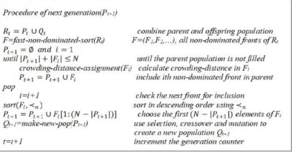
NSGA-II is a population-based metaheuristic algorithm introduced by Deb in 2001. This algorithm starts by generating an initiative population and ranking the results of the initial group. NSGA-II uses crossover and mutation operators for the exploration and exploitation of the search area. Figure 2 show the summary of the NSGA-II.
Fig 2. Pseudo code of NSGA-II algorithm
4-2- Grey wolf optimization algorithm
The GWO or Gray Wolf Optimizer algorithm is a metaheuristic method inspired from social leadership and hunting technique of grey wolves, developed by Mirjalili et al (2014). In GWO, optimization is directed by α, β, δ wolves and the rest of the wolves (ω) follow them. Grey wolves besiege their prey during hunting. Grey wolves are able to identify the hunt position and besiege it. Hence, the first three best solutions are provided to be saved. The Pseudo code of MOGWO algorithm is provided in figure 3.
𝜑 ≥ 𝛼1𝐼𝐼′𝑣∙ 𝑤𝐼𝐼′𝑣 ∀𝐼𝐼′𝑣 ∈ 𝑣1.2 (65)
𝜑 ≥ 𝛼2𝐼𝐼′𝑣∙ 𝑤𝐼𝐼′𝑣 ∀𝐼𝐼′𝑣 ∈ 𝑣1.2 (66)
41
Fig 3. Pseudo code of MOGWO algorithm
5- Numerical results
5-1- Model validation
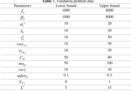
In this section, the feasibility of the model is assessed by solving the model with exact solvers. In this regard, the linearized version of the model is solved by GAMS using CPLEX solver. Due to the multi objective nature of the problem, the model is divided into three sub-problems. Each sub- problem is comprised of a single objective function; the rest of constraints are included in the proposed sub-problems. The number of distribution centers is equal to 3, backup centers are numbered 4, 5, 6, and finally, there exist 3 customers numbered from 7 to 9. Other related data are generated randomly with the upper and lower limits specified in table 7.
Table 7. Validation problem data
Parameters Lower bound Upper bound
k
f 1000 8000
k
ff 1000 8000
2 i
10 20
k
h 10 30
k
f 10 50
1
costokv 10 30
1 okv
tr 10 30
I I
C 50 80
k k
mo 50 100
k
t
cos 10 30
k
safety 0.1 0.3
2 ~
v I
I
0 1
L 5 15
42
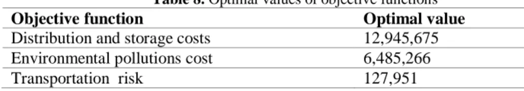
Table 8. Optimal values of objective functions
Objective function Optimal value
Distribution and storage costs 12,945,675 Environmental pollutions cost 6,485,266
Transportation risk 127,951
Figure 4 illustrates the optimal solution of the problem. According to the results, the relationships between the nodes in the network are logical. The model assigns only one backup center to the system and connects the retailers to two distribution centers. This structure makes a balance between different costs of the system.
Fig 4. Optimal solution of the problem
5-2- Solution representation scheme in metaheuristic algorithms
To use a metaheuristic algorithm for solving a given problem, the definition of the nominated solutions in the proposed algorithm is an important issue. In the proposed problem, each solution is composed of 6 vectors named from x1 to x6, containing continuous values between 0 and 1.
Vector 𝑿𝟏: Shows the visiting priority of customers.
Vector 𝑿𝟐: Demonstrates the customer allocation to DCs.
Vector 𝑿𝟑 : Is related with the allocation of customers to vehicles. Cells with value from 0 to 1/V are allocated to vehicle 1, cells with value from 1 𝑉⁄ to 2 𝑉⁄ are allocated to vehicle 2.
Vector 𝑿𝟒: Shows the allocation of DCs to backup centers.
Vector 𝑿𝟓: Indicates the number of visiting conducted by a vehicle. Each cell contains a value implying a DC has been visited.
Vector 𝑿𝟔: Determines which vehicle is allocated to each DC in level one.
By Determining the vector 𝑋4 and 𝑋6, the number of items sent to each DC is calculated taking into consideration the vehicle capacity. Thereafter, the shortage possibility is calculated. Figure 5 illustrates an instance of the designed chromosome.
43
Fig 5. Representation of a chromosome of problem solution
5-3- Parameter tuning
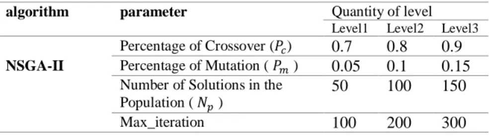
To tune the parameters of the algorithms and improve the performance of the algorithms, a Taguchi method is utilized. The nominated values for the major factors of NSGA-II are provided in table 9 according to (Rabbani et al, 2018).
Table 9. value levels of Parameters for NSGA-II algorithm
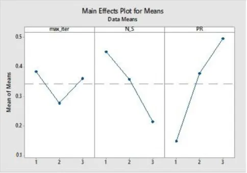
Figure 6 provides the results of Taguchi method.
In addition, the suggested values for parameters of MOGWO are provided in table 10.
Table 10. Parameters and their value levels for MOGWO algorithm
algorithm parameter Quantity of level
Level1 Level2 Level3
NSGA-II
Percentage of Crossover (𝑃𝑐) 0.7 0.8 0.9
Percentage of Mutation ( 𝑃𝑚 ) 0.05 0.1 0.15
Number of Solutions in the Population ( 𝑁𝑝 )
50 100 150
Max_iteration 100 200 300
algorithm parameter Quantity of level
Level1 Level2 Level3
MOGWO
Number of search agent ( 𝑁𝑠 ) 10 20 50 Change position rate ( 𝑃𝑟 ) 0.1 0.2 0.3
44
Fig 6. Comparison of the mean of the answers for the NSGA-II algorithm
Figure 7 depicts the related results of Taguchi method for MOGWO algorithm too.
Fig 7.Comparison of the mean of the answers for the MOGWO algorithm
6- Comparative results
Considering the multi-objective nature of the problem, some factors are defined to compare the results of proposed metaheuristic algorithms described as follows.
Max spread (DM): This metric show how the pareto answers are scattered. Larger values of this metric, indicate that algorithm have high efficiently:
45
𝐷𝑀 = √∑(𝑚𝑖𝑛𝑓𝑖− 𝑚𝑎𝑥𝑓𝑖)2 𝑛
𝑖=1
(71)
Mean ideal distance (MID): The value of this metric is related to the distance between pareto points and the ideal point. The lower value of this metric show that algorithm have better performance:
𝑀𝐼𝐷 =
∑ √( 𝑓1𝑖−𝑓1𝑏𝑒𝑠𝑡
𝑓1𝑡𝑜𝑡𝑎𝑙𝑚𝑎𝑥 −𝑓1𝑡𝑜𝑡𝑎𝑙𝑚𝑖𝑛 ) 2
+ ( 𝑓2𝑖−𝑓2𝑏𝑒𝑠𝑡
𝑓2𝑡𝑜𝑡𝑎𝑙𝑚𝑎𝑥 −𝑓2𝑡𝑜𝑡𝑎𝑙𝑚𝑖𝑛 ) 2 𝑛
𝑖=1
𝑛
(72)
The rate of achievement to objective simultaneously (RAS): This metric makes a balance between goals.
𝑅𝐴𝑆 =
[|𝑓1𝑖(𝑥)−𝑓1𝑖𝑏𝑒𝑎𝑡(𝑥)
𝑓1𝑖𝑏𝑒𝑎𝑡(𝑥) |+|
𝑓2𝑖(𝑥)−𝑓2𝑖𝑏𝑒𝑎𝑡(𝑥) 𝑓2𝑖𝑏𝑒𝑎𝑡(𝑥) |]
𝑛
(73) To compare the performance of the developed algorithms based on the given metrics, 19 problem instances (numerical examples) in different sizes are generated and the related results are included in Appendix A.Tables 11 and 12 summarize the results of NSGA-II and MOGWO respectively.
Table 11. NSGA-II algorithm output for 19 numerical examples
NSGA-II Solution
time
No# MID Max spread SM NPS RAS SNS
1 2128.402 1948.62643 388.3026 99 0.451629 337.138 19.6 2 9901.841 2994.92402 947.1654 97 0.343909 1327.495 24.8 3 14960.24 4251.83043 1626.795 97 0.183981 1424.479 26.9 4 26614.19 4859.99894 656.5366 100 0.224434 2013.4 34.8 5 43885.55 7192.19064 3292.813 95 0.268187 2982.944 39.7 6 65925.99 5793.68036 1670.296 98 0.033118 3692.972 45.6 7 170150.2 27237.3369 7986.59 98 0.161788 6394.361 51.7 8 252032.8 13156.2508 5583.598 99 0.105741 4870.001 62.7 9 284951.5 34799.2004 16779.53 95 0.212974 9177.958 63.8 10 381924 10841.6594 15844.87 96 0.083745 4170.522 67.4 11 407187.7 15401.8929 13023.62 97 0.169853 5017.187 73.5 12 511353.5 31636.8040 22114.78 96 0.111687 6296.453 78.9 13 564882.1 19289.8738 23743.56 96 0.084279 5480.24 84.9 14 1018173 13870.8791 21063.69 98 0.082837 4831.171 95.1 15 1135045 38126.7724 46694.52 96 0.116901 6484.229 102.1 16 1384478 48452.8222 57609.56 96 0.124858 11310.78 116.3 17 1843051 29375.6547 6594.312 100 0.110827 7245.205 121.9 18 2187982 122226.418 74481.82 97 0.203288 25578.92 127.3 19 2324567 30865.7246 25490.3 99 0.076859 8181.96 138.6
46 The results for MOGWO are provided in table 12, as well.
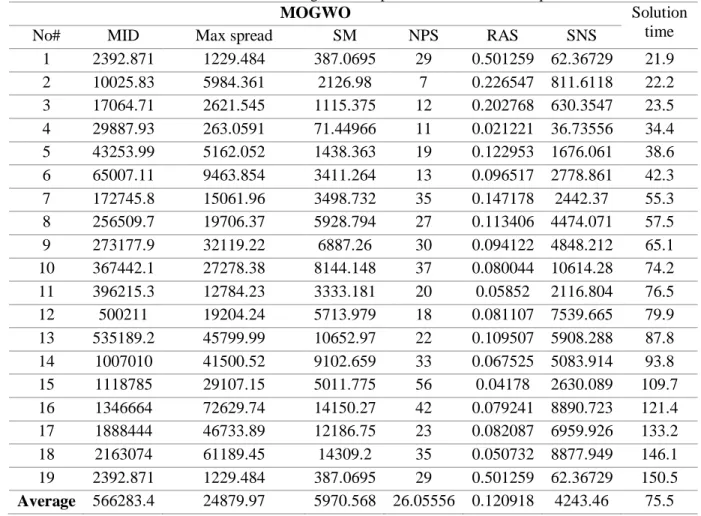
Table 12. MOGWO algorithm output for 19 numerical examples
MOGWO Solution
time
No# MID Max spread SM NPS RAS SNS
1 2392.871 1229.484 387.0695 29 0.501259 62.36729 21.9 2 10025.83 5984.361 2126.98 7 0.226547 811.6118 22.2 3 17064.71 2621.545 1115.375 12 0.202768 630.3547 23.5 4 29887.93 263.0591 71.44966 11 0.021221 36.73556 34.4 5 43253.99 5162.052 1438.363 19 0.122953 1676.061 38.6 6 65007.11 9463.854 3411.264 13 0.096517 2778.861 42.3 7 172745.8 15061.96 3498.732 35 0.147178 2442.37 55.3 8 256509.7 19706.37 5928.794 27 0.113406 4474.071 57.5 9 273177.9 32119.22 6887.26 30 0.094122 4848.212 65.1 10 367442.1 27278.38 8144.148 37 0.080044 10614.28 74.2 11 396215.3 12784.23 3333.181 20 0.05852 2116.804 76.5 12 500211 19204.24 5713.979 18 0.081107 7539.665 79.9 13 535189.2 45799.99 10652.97 22 0.109507 5908.288 87.8 14 1007010 41500.52 9102.659 33 0.067525 5083.914 93.8 15 1118785 29107.15 5011.775 56 0.04178 2630.089 109.7 16 1346664 72629.74 14150.27 42 0.079241 8890.723 121.4 17 1888444 46733.89 12186.75 23 0.082087 6959.926 133.2 18 2163074 61189.45 14309.2 35 0.050732 8877.949 146.1 19 2392.871 1229.484 387.0695 29 0.501259 62.36729 150.5 Average 566283.4 24879.97 5970.568 26.05556 0.120918 4243.46 75.5
Figure 8 illustrates that that MOGWO outperforms NSGA-II in terms of MID metric.
Fig 8. Comparison between the algorithms in terms of MID metric
The average of DM metric is equal to 5162 and 24879 for NSGA-II and MOGWO, respectively. Figure 9 provides the values of this metric for all the problem instances solved by both of the algorithms. Due to the characteristics of DM, MOGWO algorithm has a better performance than NSGA-II in terms of this
0 500000 1000000 1500000 2000000 2500000
1 3 5 7 9 11 13 15 17 19
MID
MOGWO NSGA II
47
metric. The data of table 10 and 11 show that the mean value of RAS metric for NSGA-II is 0.165 and for MOGWO algorithm is 0.12. As evident from the figure 10, MOGWO gives lower values for most of the test problems which demonstrates it has better performance in comparison with NSGA-II algorithm, regarding RAS metric formulation.
Fig 9. Comparison between the algorithms in terms of DM metric
Fig 10. Comparison between the algorithms in terms of RAS metric
The results show that the mean of run time for NSGA-II algorithm is 72.4 seconds, while MOGWO takes 75.5 seconds to solve the problem in average. Figure 11 compares the solving time for NSGA-II against MOGWO algorithm.
0 20000 40000 60000 80000 100000 120000 140000
1 2 3 4 5 6 7 8 9 10 11 12 13 14 15 16 17 18 19
DM
MOGWO NSGA II
0 20 40 60 80 100 120
1 2 3 4 5 6 7 8 9 10 11 12 13 14 15 16 17 18 19
RAS
MOGWO NSGA II
48
Fig11. Comparison between solving time of the both algorithms
As figure 12 represents, solving time metric is similar for both of the algorithms in the most of the test problems. However, MOGWO takes more run time for large-sized instances.
7- Discussion
In this section the behavior of the model is assessed to extract managerial insights for the model. In this regard, a Beverage production and distribution company around the Tehran is selected to implement the model in a real situation. The introduced company has about 300 personnel. Decreasing the related costs, reliability of delivery system and environmental issues due to governmental legislation are the major concerns of the company. The proposed company is comprised of 10 major customers, 3 DCs, and 3 backup centers. Considering the features of the company, the demand of items follows a normal distribution with range of [20,150] and [10,20]. Also, Transportation and ordering costs are generated randomly between [10,80] and [10,30]. The main parameters of the mathematical model include the risk of route, emission coefficient as well as cost parameters and lead time. Hence, the effects of changing the given parameters on the objective functions, is assessed. Figure 12 depicts the location of suppliers, retailers, DCs and BDCs in the proposed case.
0.0 20.0 40.0 60.0 80.0 100.0 120.0 140.0 160.0
0 5 10 15 20
Run time
MOGWO NSGA II
49
Fig 12. The number of routes, DCs and BDCs
Fig 13. Trend of the objective functions under changes to risk of the route
Figure 13 represents the effect of changing the risk of the route on three objective functions simultaneously. According to the results, increasing the value of risk of the route parameter leads to a sharp increment of the third objective function. The slope of the increase in the third objective function reaches its highest value when the parameter enhances from 20 percent to higher values. By increasing the risk factor, the fuel consumption of vehicles increases and the amount of emission enhances during the
0 2000 4000 6000 8000 10000 12000 14000 16000 18000 20000
0 0.2 0.4 0.6 0.8 1 1.2
50
shipment of items. In addition, the transportation cost between nodes increases leading to raise in the total cost of the system.
Fig 14. Trend of the objective functions under changes to the pollutants emission coefficient
Figure 14 shows the increasing trend for the second objective function under changing the emission parameter. The sharpest slope of the second objective function is when the parameter increases to 90 percent. The reason for this behavior is that the considered parameter is regarded in different sections of the second objective function. There are two main reasons for increasing the pollution parameters, firstly the number of vehicles has reduced and their carrying capacity has increased. Secondly, the routes with less distance are selected. The model tends to reduce the route risk, so the total cost of the system shows an increasing trend.
Fig 15. sensitive analysis for holding cost changes on objective functions
Figure 15 indicates that increasing the holing cost of the model leads to higher values of total cost. Since enhancing the holing cost, leads to higher amounts of service level and vehicle number.
0 2000 4000 6000 8000 10000 12000 14000 16000
0 0.2 0.4 0.6 0.8 1 1.2
obj func 1 obj func 2 obj fun 3
0 2000 4000 6000 8000 10000 12000 14000 16000 18000
0 20 40 60 80 100 120
51
Fig 16. Sensitivity analysis for the number of DCs
The results of figure 16 show that, with a raise in the number of DCs, the total cost of the system increases. But the slope of increment is slowly and the reason is that by increasing the number of DCs, the model decides to ship the items to more near DCs. Thus, the shipping costs are decreased and as a result, with increasing the number of DCs, the risk of the route shows an increasing trend while reducing the emissions behaves conversely.
Fig 17. Sensitivity analysis for change of lead time
0 5000 10000 15000 20000 25000
2 3 4 5 6 7 8 9 10 11
Obj func 1 Obj func 2 rout risk
0 2000 4000 6000 8000 10000 12000 14000 16000
0 5 10 15 20 25 30
52
Fig18. effect of lead time changing on inventory holding cost, safety stock, shortage cost
Figure 17 and 18 illustrate the effect of increasing the lead time on the changing trend of inventory holding, safety stock, shortage and total costs. Based on the results, one can see that enhancing the value of safety stock leads to higher amounts of inventory holding cost and lower amount of shortage cost. As a result, the total cost and service level of the system show an increasing trend. In addition, the risk of the routes has increased too.
Fig19. Sensitivity analysis for the number of BDCs
The results of figure 19 show that, with increase in the number of BDCs, the total cost of the system enhances. The main reason is that with raise in the number of BDCs, the cost of deploying these centers, and the transportation cost of BDCs increases simultaneously. On the other hand, the cost of pollution caused by the establishment and operational actions of these centers has also increased. In addition, the inventory holding costs in these centers should be considered. As a result, with increasing the number of BDCs, the emission and risk of the route shows an increasing trend.
0 20 40 60 80 100 120
0 5 10 15 20 25 30
safety stock hold inventory cost shortage cost
0 5000 10000 15000 20000 25000 30000 35000
0 2 4 6 8 10 12
Obj func 1 Obj func 2
53
Based on the results, it can be concluded that the establishment of BDCs is economically justified if the products are appealing for the customers and their related shortage causes high costs to the organization. On the other hand, inventories are the important factor in an organization and due to relatively high investment; inventories need more careful planning and control. Thus, decision makers should set a balance in the system considering according to the level of inventories. Since decision makers and managers cannot control the demand under normal circumstances, the best way to manage the inventory costs is by paying attention to the time and amount of new orders and number of items that should be held for the next periods.
8- Conclusion
In this study, a SCN comprising of suppliers, distribution centers and customers (or retailers) is designed. In addition, this study introduces a new location-inventory-routing model for supply chain network design by determining the related decisions of distribution and backup centers establishment. The proposed multi objective model includes shortage of inventory, allocation of customers to distribution centers, routing decisions, establishing new centers, and backup strategies. The model aims to reduce the related costs, environmental pollutions and transportation risks at the same time. As on of the main contributions of the current study, different factors were detected affecting the shipment risks of the system. In this regard a fuzzy TOPSIS method was applied to rank the related factors of shipment risks. Considering the time windows was another contribution of the proposed the model. In the next step, the results of the exact solver were compared with the results of the proposed metaheuristic algorithms for small-sized test problems to ensure about the performance of the metaheuristic algorithms and feasibility of the model. In addition, large-scale problems were solved by two metaheuristic algorithms namely NSGA-II and MOGWO and the results were compared. According to the comparative results, the MOGWO algorithm was able to reach results with better qualities, however, the NSGA-II had shorter run time for large-sized test problems. In addition, a sensitivity analysis was conducted on a real case to assess the behavior of the model and shows the applicability of the model in the real cases. According to the results, increasing the holding cost affects the model with grater slope compared to increasing the number of DCs. For future studies, considering soft and hard time window simultaneously or separately, regarding direct transportation from supplier to customer in case of large demand of the customer are suggested.
Reference
Abu Seman, N.A., Govindan, K., Mardani, A., Zakuan, N., Mat Saman, M.Z., Hooker, R.E., &Ozkul. S. (2019). The mediating effect of green innovation on the relationship between green supply chain management and environmental performance. Journal of Cleaner Production.
Abbasi-Parizi, S., Aminnayeri, M., & Bashiri, M. (2018). Robust solution for a minimax regret hub
location problem in a fuzzy-stochastic environment. Journal of Industrial & Management
Optimization, 14(3), 1271-1295.
Ahmadi-Javid, A., &Seddighi, A. (2012). A location-routing problem with disruption risk. Transportation Research Part E: Logistics and Transportation Review, 53:6382, 2013.
Ahmadi-Javid, &Seddighi, A. (2011). A location-routing problem for designing multisource distribution networks. Engineering optimization.
54
Amiri-Aref, M., Klibi, W., &Zied Babai, M. (2017). The multi-sourcing location inventory problem with stochastic demand. European Journal of Operational Research. 266 (2018) 72–87.
Diabat, A., Battaia, O., &Nazzal, D. (2015). An Improved Lagrangian Relaxation-based Heuristic a joint Location-Inventory problem. Computer & Operational Research.
Dehghani, E., Behfar, N., &Jabalameli, M.S. (2016). Optimizing location, routing and inventory decisions in an integrated supply chain network under uncertainty. Journal of Industrial and Systems Engineering. Vol. 9, No. 4, pp 93-111.
Dukkanci, O., Bahar Y. Kara, &Tolga Bektasü, T. (2019). The Green Location-Routing Problem. Computers and Operations Research.
Fang, C., &Zhang, J. (2018). Performance of green supply chain management: A systematic review and meta-analysis. Journal of Cleaner Production.
Guido J.L. Michelia, &Fabio Mantella. (2018). Modelling an environmentally-extended inventory routing problem with demand uncertainty and a heterogeneous fleet under carbon control policies. International Journal of Production Economics 204 (2018) 316–327.
Guo, H., Li, C., Zhang, Y., Zhang, C., &Wang, Y. (2018). A Nonlinear Integer Programming Model for Integrated Location, Inventory, and Routing Decisions in a Closed-Loop Supply Chain. Research Article. Hindawi.
Liu, S. C., &Lee, S. B. (2003). A two-phase heuristic method for the multi-depot location routing problem taking inventory control decisions into consideration. International Journal Advance Manufacturing Technology. 22(11-12): 941–950.
Liu, S. C., &Lee, S. B. (2005). A heuristic method for the combined location routing and inventory problem. Int J Adv Manuf Technol 26: 372-381.
Mallani, K.T., &Sowlati, T. (2017). Sustainability aspects in Inventory Routing Problem: A review of new trends in the literature. Journal of Cleaner Production.
Mirjalali, S.A., Mirjalali, S.M., &Saremi, S. (2016). Multi-objective grey wolf optimizer: A novel algorithm for multi-criterion optimization. Expert Systems with Applications.106–119.
Momenikia, M., Sadoullah, S., &Vahdani, B. (2018). A BI-OBJECTIVE MATHEMATICAL MODEL FOR INVENTORY-DISTRIBUTION- ROUTING PROBLEM UNDER RISK POOLING EFFECT: ROBUST META- HEURISTICS APPROACH. Economic Computation and Economic Cybernetics Studies and Research. Issue 4/2018; Vol. 52: 257-274.
Niakan, F., &Rahimi, M. (2015). A multi-objective healthcare inventory routing problem; a fuzzy possibilistic approach. Transportation Research Part E 80 (2015) 74–94.
Rau, H., Budimana, S.D., &Widyadanab, G.A. (2018). Optimization of the multi-objective green cyclical inventory routing problem using discrete multi-swarm PSO method.Transportation Research Part E 120 (2018) 51–75.
Yang, J., &Sun, H. (2015). Battery swap station location-routing problem with capacitated electric vehicles. Computers & Operations Research.