problems with a computer. The term "algorithm", used for a systematic procedure that solves a problem, is defined as a step by step solution to a problem in terms of the actions to be taken and the order in which they are to be taken. A computational physi-cist or numerical analyst often is interested in determining which of several algorithms that can solve the problem is, in some sense, the most efficient. Efficiency may be measured in many ways some of which include the number of steps in the algorithm, the time taken by the computer to execute the algo-rithm, the amount of computer memory used, among others. A major advantage of numerical analysis is that a numerical
solu-INTRODUCTION
Java is a modern object oriented language which facilitates disciplined approach to program design (Deitel and Deitel, 2007). It has features that make it suitable for mod-ern day computation which include multi-threading (parallel programming), object orientation, support for internet, among others.
Computational Physics seeks numerical so-lutions to physical problems. It involves the use of numerical analysis methods to pro-vide approximate solutions to problems in Physics. As described by Gerald and Wheat-ley (1999) numerical analysis is the develop-ment and study of procedures for solving
IMPLEMENTATION OF THE ROOT BISECTION
COMPUTATIONAL PHYSICS METHOD FOR THE
DETERMINATION OF ROOTS OF NON-LINEAR
EQUATIONS USING JAVA
1.*V. MAKINDE, 1.A.O.MUSTAPHA, 1I.C. OKEYODE, 1.F.G. AKINBORO, 1.O.S.
ADESINA AND 2.J.O. COKER
1.Department of Physics, Federal University of Agriculture, Abeokuta 2.Department of Physics, Lagos State Polytechnic, Ikorodu, Lagos
*Corresponding Author r [email protected] Tel: +2348035994001
Journal of Natural Science, Engineeringand Technology
ISSN:
Print - 2277 - 0593 Online - 2315 - 7461 © FUNAAB 2012
ABSTRACT
Advancement in programming and language development has made possible improved efficiency and accuracy in solving numerical problems and hence the numerical computation of physical problems as used in Computational Physics. Hitherto, languages such as Basic, Fortran, C, among others, have commonly been employed in solving numerical problems. In this work, Java, a modern object oriented language was deployed in solving some physical problems, specifically, determination of roots of non-linear equations using the Root-Bisection Method. A comparison between results obtained showed faster convergence and greater accuracy using Java than as obtained using Fortran.
tion can be obtained even when a problem has no analytical solution.
It is important to realize that numerical analysis of a problem always give numerical solution. Analytical methods usually give a result in terms of mathematical functions that can then be evaluated for specific in-stances (Gupta, 2010). Furthermore, a nu-merical solution is an approximation whose results can be made as accurate as desired (Arfken et al., 2012).
Solving for the roots of non-linear equa-tions is one of the numerous operaequa-tions that numerical analysis can do (Gerald and Wheatley, 1999). It can also be applied in solving large systems of linear equations; obtaining the solutions of a set of non-linear equations, interpolating to find inter-mediate values within a table of data, find-ing efficient and effective approximations of functions, among others.
Pang (2006) used Java extensively to imple-ment computational methods in his bid to introduce students to computational physics and to show the suitability of Java to com-putational science. Stroud and Booth (2001, 2003), enumerated the numerous ways in which computational methods can be adapted to solve numerical problems. In this work, Java was used to implement the computational methods because i) much of the work that had been done
in the field of computational physics used FORTRAN and C;
ii) these two languages, although still pow-erful and efficient, tend toward becom-ing old languages in that they do not provide fully for the needs of the mod-ern day computational physicists. iii) Java is a modern object oriented
lan-guage which facilitates a disciplined ap-proach to program design.
Some of the other features of Java that make it suitable for modern day computation in-clude multithreading (parallel programming), object orientation, support for the internet among others.
This work involves the:
i) implementation of the root bisection method for practically simple equations, using Java in the determination of roots of non-linear equations;
ii) testing the implemented method with examples obtained from academic sources; and
iii) evaluating the Java implementation of the computational physics methods by comparing them with similar implemen-tations done with other programming languages.
METHODOLOGY
Determination of the roots of non-linear equations
What does it mean to find the root of an equation?
Consider a function f(x); if f(x) = 0, then the values of the variable x that satisfies f(x) = 0 are called the roots of the equation. They are also known as the zeros of f(x).
Some equations are very easy to solve, that is, to find the roots. For example, if the function f(x) is linear in nature and given as f (x) = 6x - 12, then by making f(x) = 0, that is, 6x - 12 = 0, the equation is solved simply by rearranging the terms of the equation to make the variable x stand alone on the left-hand side of the equation, giving 6x = 12 or x = 12 / 6, that is, x = 2.
Also, if f(x) is quadratic, that is, f(x) = ax2 +
bx + c, in which the highest power of the
variable x in the function is 2, a formula exists to find the roots of the equation - the well known quadratic formula given as: However, as we move higher in the power to which the variable x is raised, finding the roots of the equation becomes more tedious.
According to Gerald & Wheatley (1999), it has been proved that no general formula exists for polynomials of degree greater than four meaning that there is no way to exhibit the roots in terms of "ordinary" functions. Usually, such polynomials are solved by successive approximations and some of the methods employed include: Root Bisection (or Interval Halving), Secant Method, Regula Falsi method, Fixed-Point Iteration method, Newton's method, Mul-ler's method, among others (Dass, 2010).
Theory of the Root Bisection Method
The root bisection method is an ancient but effective method for finding a zero of f(x). Out of the common methods, the root bi-section method is almost the simplest to understand and the easiest to implement. To find a root of f(x), the root bisection method begins with two values x = x1 and x
= x2 that bracket (enclose) a root. It is
known that a root is enclosed if the func-tion changes sign at the endpoints, that is, at f(x1) and f(x2); this is true if (f(x1)*f(x2)) <
0 (Kreszig, 2006). It is certain that there is at least one root in the interval [x1, x2] as
long as f(x) is continuous in [x1, x2]. The
method then successively divides the inter-val in half and replaces one endpoint with the midpoint so that again the root is en-closed. Known in advance is that the error in the estimate of the root must be less than |(x2–x1)*(1/2n)| where n is the number of
iterations performed (Gupta, 2010).
In implementing the Root Bisection Method, the pseudocode was written to set the brack-et values and algorithm for implementation. The pseudocode for the Root Bisection algo-rithm is stated thus.
To determine a root of f(x) = 0 that is accu-rate within a specified tolerance value, given values X1 and X2 such that f(X1) * f(X2) < 0.
REPEAT
Set X3 = (X1 + X2) / 2 IF (f(X3) * f(X1) < 0): Set X2 = X3 ELSE Set X1 = X3 END IF
UNTIL (|X1 - X2| < 2 * tolerance value) or f(X3) = 0
NOTE: The method may give a false root if f(x) is discontinuous in [X1, X2]. The final value of X3 approximates the root within the accuracy of the specified tolerance value (Gerald & Wheatley, 1999).
Implementation
Implementation of the root bisection meth-od was achieved by creating a Java class called RootBisection. This class consists of six private fields and fifteen public methods which includes a constructor and the corre-sponding set and get assessors for each of the fields. The method called getRoot() imple-ments the algorithm for the root bisection method.
A driver class called RootBisectionMethod (Adesina, 2010), was created to collect the data to satisfy the preconditions of the root
bisection algorithm and to execute the getRoot() method of the RootBisection class which is the method that implements the root bisection algorithm. The
RootBisection-Method class is an application class because it contains a method called main() which is the entry point for all Java programs. The code listing for the getRoot() method is shown next.
V. MAKINDE, .A.O.MUSTAPHA, .C. OKEYODE, F.G. AKINBORO, .O.S. ADESINA AND J.O. COKER
1 publicdouble getRoot() {
2 int iterate = 0;
3 double mid, x1, x2, oppSign, fxmid;
4 x1 = lowerLimitOfInterval; 5 x2 = upperLimitOfInterval; 6 setOutput("");
7 compileOutput(String.format("\n%15s%15s%15s%15s%15s\n", "ITR NO","X1", "X2", "X3", "F(X3)"));
8 do {
9 iterate += 1;
10 mid = (x2 + x1) / 2;
11 fxmid = Function.getFofX(mid, coefficients);
12 compileOutput(String.format("\n%15d%15.7f%15.7f%15.7f %15.7f", iterate, x1, x2, mid, fxmid));
13 oppSign = fxmid * Function.getFofX(x1, coefficients); 14 if ( oppSign < 0 ) {
15 x2 = mid;
16 } else {
17 x1 = mid;
18 }
19 } while ( !((Math.abs(x1 - x2) < ( 2 * tolerance )) ||
(fxmid == 0) || (iterate >= maxIteration)) );
20 compileOutput(String.format("\n\n%s\n\n", "Program output for x1 = " +
lowerLimitOfInterval + ", x2 = " + upperLimitOfInterval + ", tolerance = " + tolerance));
21 return mid;
22 }
Code Listing 1: The getRoot() method of RootBisection class
Lines 2 and 3 of Code Listing 1 declare var-iables that are used within the getRoot() method. Integer variable iterate (which is initialized to zero) keeps track of the num-ber of iterations. Variables mid, X1, X2, oppSign, and fxmid are of double data-type
and they store double precision floating point numbers; .mid stores the mid-point of the interval [X1, X2], while X1, X2 stores the lower and upper limits of the interval respectively.
The root bisection algorithm starts from line 8 and ends at 19 of Code Listing 1. Line 11 calls method getFofX() of class Function which contains only two methods -getFofX() and getDerivativeFofX(). getFofX() computes the value of the polynomial func-tion using the value of x and the coeffi-cients vector passed to it as arguments; com-pileOutput() is one of the methods of the root bisection class; it stores the format-ted output, which will be displayed to the user, passed to it as arguments as it is used in lines 7 and 20. Line 13 performs the op-eration f(X3) * f(X1) and stores the result in the variable oppSign. Line 14 begins an if-else structure that tests whether f(x) changes sign at the endpoints X3 and X1. If the
function changes sign then mid replaces X2 in line 15 else mid replaces X1 in line 17. The condition in line 19 checks if the abso-lute value of X1 - X2 (Math.abs(X1 - X2)) is not less than 2 times the tolerance value giv-en or if f(X3) (fxmid) is not equal to zero or if the iteration number is not greater than or equal to the maximum given. If this complex logical condition is true, that is if any one of the tests is true, then the iteration continues otherwise lines 20 and 21 execute. Line 21 returns the value of X3 that is mid.
In order to obtain the roots therefore, pa-rameters are first set as input to the program thus: For a polynomial of order n,
f(x) = Anxn + An-1xn-1 + An-2xn-2 + …….. + A2x2 + A1x + A0
For example, if f(x) = x2 – 2; then A2 = 1, A1 = 0, and A0 = - 2
if f(x) = x3 + x2 - 3x – 3, then A3 = 1, A2 = 1, A1 = - 3, and A0 = - 3
if f(x) = x4 – 2; then A4 = 1, A3 = 0, A2 = 0, A1 = 0, and A0 = - 2
WELCOME TO THE ROOT BISECTION METHOD
THIS PROGRAM IMPLEMENTATION ALLOWS YOU TO FIND THE ROOT(S) OF A POLYNOMIAL OR NON-LINEAR EQUATION
Enter the lower limit of the interval x1: Enter the upper limit of the interval x2: Enter the degree of the polynomial: n
Now, enter the elements of the coefficient vector one after the other. Enter A0:
Enter A1:
Enter A2:
. . Enter An-1:
Enter An:
Enter the tolerance value: 0.00001
Enter the maximum number of iterations in case tolerance is not met: 20 In order to determine other roots, either of
two approaches can be made: i) to reset the interval limits to new values of [x1, x2]
which bracket the second root; ii) to set an all encompassing enclosing limits [X1, X2] from the outset.
Tests and Results
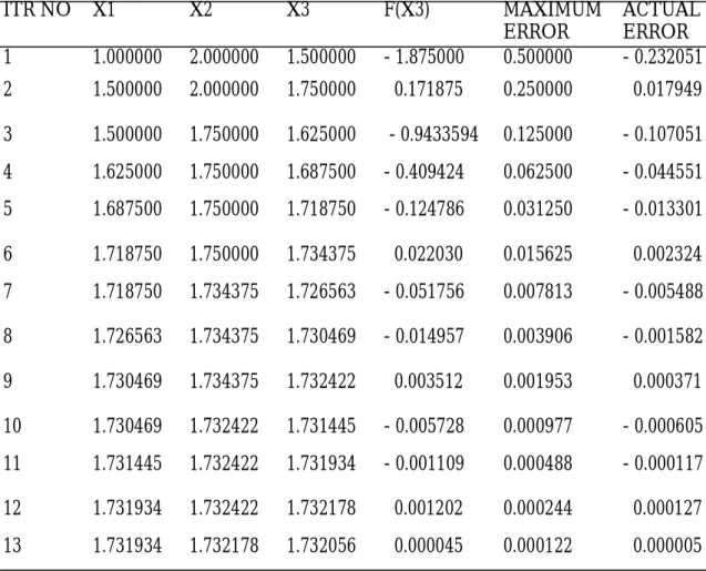
Example 1: As an example, consider the following function from Gerald & Wheatley (1999): f(x) = x3 + x2 - 3x - 3 = 0.
It can almost be seen by inspection that a root is Ö3, that is, square root of 3. Alt-hough the function is simple enough to be
easily solved by hand, it is a good example to show how successive iterates converge on the value Ö3, that is, 1.732050808.The result obtained by Gerald & Wheatley (1999), who implemented the Root Bisection Method using FORTRAN 90 is given next in Table 1:
V. MAKINDE, .A.O.MUSTAPHA, I.C. OKEYODE, F.G. AKINBORO, O.S. ADESINA AND .J.O. COKER
Table 1: Finding the root of f(x) = x3 + x2 - 3x - 3 = 0 starting with X1 = 1, X2 = 2,
and tolerance 1E-4 by root bisection method (Adapted from Gerald & Wheatley, 1999)
ITR NO X1 X2 X3 F(X3) MAXIMUM
ERROR
ACTUAL ERROR 1 1.000000 2.000000 1.500000 - 1.875000 0.500000 - 0.232051 2 1.500000 2.000000 1.750000 0.171875 0.250000 0.017949 3 1.500000 1.750000 1.625000 - 0.9433594 0.125000 - 0.107051 4 1.625000 1.750000 1.687500 - 0.409424 0.062500 - 0.044551 5 1.687500 1.750000 1.718750 - 0.124786 0.031250 - 0.013301 6 1.718750 1.750000 1.734375 0.022030 0.015625 0.002324 7 1.718750 1.734375 1.726563 - 0.051756 0.007813 - 0.005488 8 1.726563 1.734375 1.730469 - 0.014957 0.003906 - 0.001582 9 1.730469 1.734375 1.732422 0.003512 0.001953 0.000371 10 1.730469 1.732422 1.731445 - 0.005728 0.000977 - 0.000605 11 1.731445 1.732422 1.731934 - 0.001109 0.000488 - 0.000117 12 1.731934 1.732422 1.732178 0.001202 0.000244 0.000127 13 1.731934 1.732178 1.732056 0.000045 0.000122 0.000005 Tolerance met
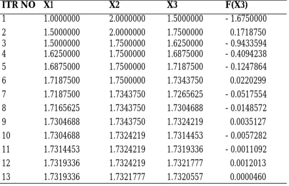
The result obtained in the implementation of the root bisection algorithm using Java (Code Listing 1) is given next in Table 2:
Tables 1 and 2 show that it takes the root bisection method thirteen iterations to find the approximate root within the accuracy of the tolerance value. X3 is the mid-point of the interval while f(X3) gives the value of the function at X3.
It was observed in the tables that the esti-mate of the root may be better at an earlier iteration than at later ones. The second iter-ate in Table 1 is closer to the true root than are the next two, that is, iterates 3 and 4. Also, it is closer at iterate 6 than iterate 7. In this example, we have the advantage of knowing the answer, but this is never the case in real world applications. However, the values of f(x) themselves show that these better estimates are closer to the root.
Although, this may not always be an absolute indicator due to the fact that some functions may be nearly zero at points which are not so near the root, but for smooth functions, a small value of the function is a good indica-tor that we are near the root; this is especially true when we are quite close to the root.
Example 2: Consider another example: f(x) = x4 - 2 = 0
This function is a fourth degree polyno-mial and a root is the fourth-root of 2 which is 1.189207115.
Using the Java implementation of the root bisection method, the following results shown in Table 3 were obtained.
Table 2: Finding the root of f(x) = x3 + x2 - 3x - 3 = 0 starting with X1 = 1, X2 = 2,
and tolerance of 1E-4 by root bisection method using Java Approximate root found: 1.732056
ITR NO X1 X2 X3 F(X3)
1 1.0000000 2.0000000 1.5000000 - 1.6750000
2 1.5000000 2.0000000 1.7500000 0.1718750
3 1.5000000 1.7500000 1.6250000 - 0.9433594
4 1.6250000 1.7500000 1.6875000 - 0.4094238
5 1.6875000 1.7500000 1.7187500 - 0.1247864
6 1.7187500 1.7500000 1.7343750 0.0220299
7 1.7187500 1.7343750 1.7265625 - 0.0517554
8 1.7165625 1.7343750 1.7304688 - 0.0148572
9 1.7304688 1.7343750 1.7324219 0.0035127
10 1.7304688 1.7324219 1.7314453 - 0.0057282
11 1.7314453 1.7324219 1.7319336 - 0.0011092
12 1.7319336 1.7324219 1.7321777 0.0012013
13 1.7319336 1.7321777 1.7320557 0.0000460
It can also be observed in Table 3, that ear-lier estimates of the root may be better as reflected in iterate 4 being closer to the root than the next two. It took thirteen iterations for the root bisection method to converge to an approximate root within the accuracy of the tolerance value, that is, 0.0001. From the foregoing, it is evident that the root bisection method is indeed slow to
converge.
Root Bisection Method Applied to Quad-ratic Equations
Hitherto, all examples taken were non-quadratic. To elucidate its applicability to quadratic equations, two quadratic equations are here taken as further examples.
Table 3: Finding the root of f(x) = x4- 2 = 0 starting with X1 = 1, X2 = 2, and
tolerance of 1E-4 by root bisection method using Java
ITR NO X1 X2 X3 F(X3)
1 1.0000000 2.0000000 1.5000000 3.0625000
2 1.0000000 1.5000000 1.2500000 0.4414063
3 1.0000000 1.2500000 1.1250000 - 0.3981934
4 1.1250000 1.2500000 1.1875000 - 0.0114594
5 1.1875000 1.2500000 1.2187500 0.2062693
6 1.1875000 1.2187500 1.2031250 0.0952845
7 1.1875000 1.2031250 1.1953125 0.0413893
8 1.1875000 1.1953125 1.1914063 0.0148350
9 1.1875000 1.1914063 1.1894531 0.0016555
10 1.1875000 1.1894531 1.1884766 - 0.0049100
11 1.1884766 1.1894531 1.1889648 - 0.0016293
12 1.1889648 1.1894531 1.1892090 0.0000126
13 1.1889648 1.1892090 1.1890869 - 0.0008085
Program output for x1 = 1.0, x2 = 2.0, tolerance = 1.0E-4
Example 3: Consider the equation f(x) = x2 – 2 = 0 (Adapted from Stroud and Booth,
2003)
Results obtained from the Root Bisection Method Java program is given as follows: Approximate root found: 1.414200
ITR NO X1 X2 X3 F(X3)
1 1.0000000 2.0000000 1.5000000 0.2500000
2 1.0000000 1.5000000 1.2500000 - 0.4375000
3 1.2500000 1.5000000 1.3750000 - 0.1093750
4 1.3750000 1.5000000 1.4375000 0.0664063
5 1.3750000 1.4375000 1.4062500 - 0.0224609
6 1.4062500 1.4375000 1.4218750 0.0217285
7 1.4062500 1.4218750 1.4140625 - 0.0004272
8 1.4140625 1.4218750 1.4179688 0.0106354
9 1.4140625 1.4179688 1.4160156 0.0051003
10 1.4140625 1.4160156 1.4150391 0.0023355 11 1.4140625 1.4150391 1.4145508 0.0009539 12 1.4140625 1.4145508 1.4143066 0.0002633 13 1.4140625 1.4143066 1.4141846 - 0.0000820 14 1.4141846 1.4143066 1.4142456 0.0000906 15 1.4141846 1.4142456 1.4142151 0.0000043 16 1.4141846 1.4142151 1.4141998 - 0.0000388 Program output for x1 = 1.0, x2 = 2.0, tolerance = 1.0E-5
Example 4::f(x) = 2x2 – 9x + 5 = 0
The first root can be found in the interval [1, 4] and the results obtained from the RootBi-sectionMethod Java program are given as follows:
Enter the lower limit of the interval x1: 1 Enter the upper limit of the interval x2: 4 Enter the degree of the polynomial: 2
Now, enter the elements of the coefficient vector one after the other. Enter A0: 5
Enter A1: -9 Enter A2: 2
Enter the tolerance value: 0.00001
Now, to find the second root, the interval limits are reset to new values of [-1, 1] which bracket the second root. The results obtained from the Root Bisection Method Java pro-gram are given below:
Enter the lower limit of the interval x1: -1 Enter the upper limit of the interval x2: 1 Enter the degree of the polynomial: 2
Now, enter the elements of the coefficient vector one after the other. Enter A0: 5
Enter A1: -9 Enter A2: 2
Enter the tolerance value: 0.00001
Enter the maximum number of iterations in case tolerance is not met: 20 Approximate root found: 3.850780
ITR NO X1 X2 X3 F(X3)
1 1.0000000 4.0000000 2.5000000 - 5.0000000 2 2.5000000 4.0000000 3.2500000 - 3.1250000 3 3.2500000 4.0000000 3.6250000 - 1.3437500 4 3.6250000 4.0000000 3.8125000 - 0.2421875 5 3.8125000 4.0000000 3.9062500 0.3613281 6 3.8125000 3.9062500 3.8593750 0.0551758 7 3.8125000 3.8593750 3.8359375 - 0.0946045 8 3.8359375 3.8593750 3.8476563 - 0.0199890 9 3.8476563 3.8593750 3.8535156 0.0175247 10 3.8476563 3.8535156 3.8505859 - 0.0012493 11 3.8505859 3.8535156 3.8520508 0.0081334 12 3.8505859 3.8520508 3.8513184 0.0034410 13 3.8505859 3.8513184 3.8509521 0.0010956 14 3.8505859 3.8509521 3.8507690 - 0.0000769 15 3.8507690 3.8509521 3.8508606 0.0005093 16 3.8507690 3.8508606 3.8508148 0.0002162 17 3.8507690 3.8508148 3.8507919 0.0000696 18 3.8507690 3.8507919 3.8507805 - 0.0000037 Program output for x1 = 1.0, x2 = 4.0, tolerance = 1.0E-5
Approximate root found: 0.649216
ITR NO X1 X2 X3 F(X3)
1 -1.0000000 1.0000000 0.0000000 5.0000000
2 0.0000000 1.0000000 0.5000000 1.0000000
3 0.5000000 1.0000000 0.7500000 - 0.6250000
4 0.5000000 0.7500000 0.6250000 0.1562500
5 0.6250000 0.7500000 0.6875000 - 0.2421875
6 0.6250000 0.6875000 0.6562500 - 0.0449219
7 0.6250000 0.6562500 0.6406250 0.0551758
8 0.6406250 0.6562500 0.6484375 0.0050049
9 0.6484375 0.6562500 0.6523438 - 0.0199890
10 0.6484375 0.6523438 0.6503906 0.0074997
11 0.6484375 0.6503906 0.6494141 - 0.0012493
12 0.6484375 0.6494141 0.6489258 0.0018773
13 0.6489258 0.6494141 0.6491699 0.0003139
14 0.6491699 0.6494141 0.6492920 - 0.0004677
15 0.6491699 0.6492920 0.6492310 0.0000769
16 0.6491699 0.6492310 0.6492004 0.0001185
17 0.6492004 0.6492310 0.6492157 0.0000208
Program output for x1 = -1.0, x2 = 1.0, tolerance = 1.0E-5
In another way round, the interval could be set at [-1, 4] form onset. For this example, do-ing that would yield the result as given next:
WELCOME TO THE ROOT BISECTION METHOD
THIS PROGRAM IMPLEMENTATION ALLOWS YOU TO FIND THE ROOT OF A POLYNOMIAL OR NON-LINEAR EQUATION
Enter the lower limit of the interval x1: -1 Enter the upper limit of the interval x2: 4 Enter the degree of the polynomial: 2
Now, enter the elements of the coefficient vector one after the other. Enter A0: 5
Enter A1: -9 Enter A2: 2
Enter the tolerance value: 0.00001
First Approximate root found: 0.649227
ITR NO X1 X2 X3 F(X3) 1 -1.0000000 4.0000000 1.5000000 - 4.0000000 2 -1.0000000 1.5000000 0.2500000 2.8750000 3 0.2500000 1.5000000 0.8750000 - 1.3437500 4 0.2500000 0.8750000 0.5625000 0.5703125 5 0.5625000 0.8750000 0.7187500 - 0.4355469 6 0.5625000 0.7187500 0.6406250 0.0551758 7 0.6406250 0.7187500 0.6796875 - 0.1932373 8 0.6406250 0.6796875 0.6601563 - 0.0697937 9 0.6406250 0.6601563 0.6503906 - 0.0074997 10 0.6406250 0.6503906 0.6455078 0.0237904 11 0.6455078 0.6503906 0.6479492 0.0081334 12 0.6479492 0.6503906 0.6491699 0.0003139 13 0.6491699 0.6503906 0.6497803 - 0.0035937 14 0.6491699 0.6497803 0.6494751 - 0.0016401 15 0.6491699 0.6494751 0.6493225 - 0.0006631 16 0.6491699 0.6493225 0.6492462 - 0.0001746 17 0.6491699 0.6492462 0.6492081 0.0000696 18 0.6492081 0.6492462 0.6492271 - 0.0000525 Second Approximate root found: 3.850769
ITR NO X1 X2 X3 F(X3) 1 0.6492462 4.0000000 2.3246231 -5.1138628 2 2.3246231 4.0000000 3.1623116 -3.4603753 3 3.1623116 4.0000000 3.5811558 -1.5810486 4 3.5811558 4.0000000 3.7905779 - 0.3782395 5 3.7905779 4.0000000 3.8952889 0.2889514 6 3.7905779 3.8952889 3.8429334 - 0.0501263 7 3.8429334 3.8952889 3.8691112 0.1180420 8 3.8429334 3.8691112 3.8560223 0.0336152 9 3.8429334 3.8560223 3.8494779 - 0.0083412 10 3.8494779 3.8560223 3.8527501 0.0126156 11 3.8494779 3.8527501 3.8511140 0.0021319 12 3.8494779 3.8511140 3.8502959 - 0.0031060 13 3.8502959 3.8511140 3.8507049 - 0.0004874 14 3.8507049 3.8511140 3.8509095 0.0008222 15 3.8507049 3.8509095 3.8508072 0.0001674 16 3.8507049 3.8508072 3.8507561 - 0.0001600 17 3.8507561 3.8508072 3.8507816 0.0000037 18 3.8507561 3.8507816 3.8507688 - 0.0000782 Program output for x1 = 0.6492462, x2 = 4.0, tolerance = 1.0E-5
CONCLUSION
Scientific computing is today becoming the third pillar of scientific inquiry alongside the more traditional theory and experimenta-tion pillars. For example, scientists today do not have to brave the risks of hazardous or dangerous chemical experiments, rather they use computational methods imple-mented with programming languages such as Java to simulate and model such experi-ments.
The relevance that computational physics, numerical analysis or computational science in general has today, is as a result of a lot of work that had been done in the implemen-tation of several compuimplemen-tational methods using computer programming languages. FORTRAN, which was developed by IBM, is essentially a computational tool; it has been used extensively to develop programs in both the defense and geophysical fields (Chapman, 1998). Chapman (1998) imple-mented computational methods using FORTRAN 90/95. C, a language developed by Dennis Ritchie in the 1960s, is another language that has found extensive use in computational science. C is most suitable for High Performance Computing (HPC) because of its speed of execution (Chow, 2000). However, it is very susceptible to errors especially if used by a not so skillful programmer.
The scale of modern day problems being solved by computational physicist requires the use of programming languages that are very easy to use; provide features which make it possible to re-use existing codes; is capable of specifying different operations to be executed simultaneously by the computer; and that enable distribut-ed programs to be easily developdistribut-ed (Kiusalaas, 2005; Jeffrey, 2002)). Java is
such a programming language, and has been used in this work to determine roots of non-linear equations as set out, and for adaptabil-ity in training students.
One pertinent question is, having found one of the roots, how do we obtain the other root(s)? The solution to that problem is simply that to find all roots, the limits are reset to new values within the expected range x1 < x < x2, or a broad all enclosing limits [x1, x2] is chosen from inception with the necessary codes included. Either of these procedures brings out clearly the other roots of the equation being solved.
The main advantage of root bisection is that it is guaranteed to work if f(x) is continuous in [x1, x2] and if the values x = x1 and x = x2
actually bracket a root. Another advantage is that the number of iterations required to achieve a specified accuracy is known in ad-vance (DeVries, 1993). To find all roots, the limits are reset to new values within the ex-pected range x1< x < x2, or to choose a
broad all enclosing limits [X1, X2] from in-ception.
The major drawback of root bisection is that it is slow to converge. Other methods such as the Newton's method require fewer num-bers of iterations to achieve the same level of accuracy.
In spite of arguments that other methods find roots with fewer iterations, root bisec-tion is nevertheless an important tool in the computational physicist's arsenal. It is gener-ally recommended that root bisection be used for finding approximate root which can then be refined by more efficient methods. The reason is that most other methods re-quire a starting value near to a root which, if not available, may cause them to fail com-pletely.
REFERENCES
Adesina, O.S. 2010. Implementation of
Basic Computational Physics Methods us-ing Java. Unpublished B.Sc. Project, Federal University of Agriculture, Abeokuta, Nige-ria.
Arfken, G.B., Weber, H.J., Harris, F.E.
2012. Mathematical Methods for Physicists. 7th
Edition. Associated Press. New York, U.S.A. P. 1205
Chapman, S.J. 1998. FORTRAN 90/95 for
Scientists and Engineers. McGraw-Hill, USA P. 431
Chow, T.L. 2000. Mathematical Methods for
Physicists – A Concise Introduction. Cambridge University Press. U.S.A. pp 569
Dass, H.K. 2010. Advanced Engineering
Mathematics. S Chand and Co. Publishers. New Delhi, India. pp 1358
Deitel, P.J., Deitel, H.M. 2007. Java: How
to Program. Pearson Education Inc, New Jer-sey, USA. P. 317
DeVries, P.L. 1993. A First Course in
Com-putational Physics. John Wiley & Sons, New York, U.S.A. P. 435.
Gerald, C.F., Wheatley, P.O. 1999. Applied
Numerical Analysis. Dorling Kindersley, India. P. 698.
Gupta, B.D. 2010. Mathematical Physics. 4th
Edition. Vikas Publishing House, New Delhi, India. P. 1417.
Jeffrey, A. 2002. Advanced Engineering
Mathe-matics. Academic Press. U.S.A. P. 1181
Kiusalaas, J. (2005). Numerical Methods in
Engineering with MATLAB. Cambridge Uni-versity Press. U.S.A. pp 435.
Kreyszig, E. 2006. Advanced Engineering
Mathematics. 9th Edition. John Wiley & Sons.
U.S.A. P. 1246.
Pang, T. 2006. Introduction to Computational
Physics. Cambridge University Press, New York, USA. P. 528.
Stroud, K.A., Booth, D.J. 2001. Engineering
Mathematics. Palgrave Macmillan, New York, USA. P. 1236.
Stroud, K.A., Booth, D.J. 2003. Advanced
Engineering Mathematics. Palgrave Macmillan, New York, USA. P. 1057.
(Manuscript received: 4th April, 2013 ; accepted 4th December, 2013).