44 VALIDATED PLANETS FROMK2 CAMPAIGN 10
John H. Livingston,1, 2, 3Michael Endl,4Fei Dai,5, 6 William D. Cochran,4 Oscar Barragan,7 Davide Gandolfi,7
Teruyuki Hirano,8 Sascha Grziwa,9 Alexis M. S. Smith,10 Simon Albrecht,11Juan Cabrera,10
Szilard Csizmadia,10 Jerome P. de Leon,1 Hans Deeg,12, 13 Philipp Eigm¨uller,10 Anders Erikson,10
Mark Everett,14 Malcolm Fridlund,15, 16 Akihiko Fukui,17 Eike W. Guenther,18 Artie P. Hatzes,18
Steve Howell,19 Judith Korth,9Norio Narita,1, 20, 21, 12 David Nespral,12, 13 Grzegorz Nowak,12, 13
Enric Palle,12, 13 Martin P¨atzold,9 Carina M. Persson,16 Jorge Prieto-Arranz,12, 13 Heike Rauer,10, 22
Motohide Tamura,1, 20, 21 Vincent Van Eylen,15 and Joshua N. Winn6
1Department of Astronomy, University of Tokyo, 7-3-1 Hongo, Bunkyo-ku, Tokyo 113-0033, Japan 2JSPS Fellow
4Department of Astronomy and McDonald Observatory, University of Texas at Austin, 2515
Speedway, Stop C1400, Austin, TX 78712, USA
5Department of Physics and Kavli Institute for Astrophysics and Space Research, Massachusetts Institute of Technology, Cambridge, MA,
02139, USA
6Department of Astrophysical Sciences, Princeton University, 4 Ivy Lane, Princeton, NJ 08544, USA 7Dipartimento di Fisica, Universit`a di Torino, via P. Giuria 1, 10125 Torino, Italy
8Department of Earth and Planetary Sciences, Tokyo Institute of Technology, 2-12-1 Ookayama, Meguro-ku, Tokyo 152-8551, Japan 9Rheinisches Institut f¨ur Umweltforschung an der Universit¨at zu K¨oln, Aachener Strasse 209, 50931 K¨oln, Germany
10Institute of Planetary Research, German Aerospace Center, Rutherfordstrasse 2, 12489 Berlin, Germany
11Stellar Astrophysics Centre, Department of Physics and Astronomy, Aarhus University, Ny Munkegade 120, DK-8000 Aarhus C,
Denmark
12Instituto de Astrof´ısica de Canarias, C/ V´ıa L´actea s/n, 38205 La Laguna, Spain 13Departamento de Astrof´ısica, Universidad de La Laguna, 38206 La Laguna, Spain
14National Optical Astronomy Observatory, 950 North Cherry Avenue, Tucson, AZ 85719, USA 15Leiden Observatory, Leiden University, 2333CA Leiden, The Netherlands
16Department of Space, Earth and Environment, Chalmers University of Technology, Onsala Space Observatory, 439 92 Onsala, Sweden 17Okayama Astrophysical Observatory, National Astronomical Observatory of Japan, Asakuchi, Okayama 719-0232, Japan
18Th¨uringer Landessternwarte Tautenburg, Sternwarte 5, D-07778 Tautenberg, Germany
19Space Science and Astrobiology Division, NASA Ames Research Center, Moffett Field, CA 94035, USA 20Astrobiology Center, NINS, 2-21-1 Osawa, Mitaka, Tokyo 181-8588, Japan
21National Astronomical Observatory of Japan, NINS, 2-21-1 Osawa, Mitaka, Tokyo 181-8588, Japan 22Center for Astronomy and Astrophysics, TU Berlin, Hardenbergstr. 36, 10623 Berlin, Germany
ABSTRACT
We present 44 validated planets from the 10th observing campaign of the NASA K2 mission, as well as high resolution spectroscopy and speckle imaging follow-up observations. These 44 planets come from an initial set of 72 vetted candidates, which we subjected to a validation process incorporating pixel-level analyses, light curve analyses, observational constraints, and statistical false positive probabilities. Our validated planet sample has median values ofRp = 2.2R⊕,Porb = 6.9 days,Teq= 890 K, and J= 11.2 mag. Of particular interest are four ultra-short period planets (Porb .1 day), 16 planets smaller than 2 R⊕, and two planets with large predicted amplitude atmospheric transmission features orbiting infrared-bright stars. We also present 27 planet candidates, most of which are likely to be real and worthy of further observations. Our validated planet sample includes 24 new discoveries, and has enhanced the number of currently known super-Earths (Rp ≈1–2R⊕), sub-Neptunes (Rp ≈2–4R⊕), and sub-Saturns (Rp ≈ 4–8R⊕) orbiting bright stars (J = 8–10 mag) by ∼4%,∼17%, and∼11%, respectively.
Livingston et al.
1. INTRODUCTION
TheK2 mission (Howell et al. 2014) is extending the
Kepler legacy to a survey of the ecliptic plane, enabling the detection of transiting planets orbiting a wider range of host stars. The increased sky coverage of K2 has enabled the detection of planets orbiting brighter host stars, as well as a larger selection of M dwarfs (Crossfield et al. 2016; Dressing et al. 2017; Hirano et al. 2018a). As a result, K2 is yielding a large number of promis-ing targets for follow-up studies (e.g.Vanderburg et al. 2015;Crossfield et al. 2015;Montet et al. 2015; Vander-burg et al. 2016a;Petigura et al. 2015;Vanderburg et al. 2016a,b,c;Crossfield et al. 2017). K2has also discovered planets in stellar cluster environments (Obermeier et al. 2016;Pepper et al. 2017;David et al. 2016b;Mann et al. 2016a, 2017;Gaidos et al. 2017; Ciardi et al. 2018), in-cluding one possibly still undergoing radial contraction (David et al. 2016a;Mann et al. 2016b).
We present here the results of our analysis of theK2
photometric data collected during Campaign 10 (C10), along with a coordinated campaign of follow-up obser-vations to better characterize the host stars and rule out false positive scenarios. Because of C10’s relatively high galactic latitude, blending within the photometric aper-tures is less significant than for other fields, and contam-ination from background eclipsing binaries is low. We detect 72 planet candidates and validate 44 of them as
bona fideplanets using our observational constraints, 24 of which have not previously been reported in the lit-erature. Our sample contains a remainder of 27 planet candidates, many of which are likely real planets.
The transit detections and follow-up observations that led to these discoveries were the result of an interna-tional collaboration called KESPRINT. Formed from the merger of two previously separate collaborations (KEST and ESPRINT), KESPRINT is focused on de-tecting and characterizing interesting new planet can-didates from the K2 mission (e.g.Fridlund et al. 2017;
Guenther et al. 2017;Gandolfi et al. 2017;Niraula et al. 2017;Smith et al. 2018;Dai et al. 2017;Livingston et al. 2018;Hirano et al. 2018b;Van Eylen et al. 2018).
The rest of the paper is structured as follows. In
Section 2 we describe our K2 photometry and tran-sit search. In Section 3 and Section 4 we describe our follow-up speckle imaging and high resolution spec-troscopy of the candidates from our detection and vet-ting procedures. InSection 5we describe our statistical validation framework and results. In Section 6we dis-cuss particular systems of interest, and we conclude with a summary inSection 7.
2. K2 PHOTOMETRY AND TRANSIT SEARCH
Here we describe how we produce a list of vetted planet candidates from the pixel data telemetered from the Kepler spacecraft, as well as detailed light curve analyses. Throughout this paper we refer to stars by their nine digit EPIC IDs, and we concatenate these with two digit numbers to refer to planet candidates (ordered by orbital period).
2.1. Photometry
In C10,K2 observed a∼110 square degree field near the North Galactic cap from July 06, 2016 to Septem-ber 20, 2016. Long cadence (30 minute) exposures of 28,345 target stars were downlinked from the spacecraft, and the data were calibrated and subsequently made available on the Mikulski Archive for Space Telescopes1 (MAST). During the beginning of the campaign, a 3.5 pixel pointing error was detected and subsequently cor-rected six days after the start of observations. The data during this time is of substantially lower quality than the rest of the campaign, so we discard it in our analy-sis. An additional data gap was the result of the failure of detector module 4, which caused the photometer to power off for 14 days.
2.2. Systematics
Following the loss of two of its four reaction wheels, theKepler spacecraft has been operating asK2 (Howell et al. 2014). The dominant systematic signal inK2 light curves is caused by the rolling motion of the spacecraft along its bore sight coupled with inter- and intra-pixel sensitivity variations. We used a method similar to that described by Vanderburg & Johnson (2014) to reduce this systematic flux variation. Our light curve produc-tion pipeline is as follows. We first downloaded the tar-get pixel files from MAST. We laid circular apertures around the brightest pixel within the “postage stamp” (the set of pixels of theKepler photometer correspond-ing to a given source). To obtain the centroid position of the image, we fitted a 2-D Gaussian function to the in-aperture flux distribution. We then fitted a piece-wise linear function between the flux variation and the centroid motion of target. The fitted piecewise linear function was then detrended from the observed flux vari-ation.
2.3. Transit search
Before searching the light curve for transits, we first removed any long-term systematic or instrumental flux variations by fitting a cubic spline to the reduced light curve from the previous section. To look for periodic
transit signals, we employed the Box-Least-Squares al-gorithm (BLS, Kov´acs et al. 2002). We improved the efficiency of the original BLS algorithm by using a non-linear frequency grid that takes into account the scaling of transit duration with orbital period (Ofir 2014). We also adopted the signal detection efficiency (SDE, Ofir 2014) which quantifies the significance of a detection. SDE is defined by the amplitude of peak in the BLS spectrum normalized by the local standard deviation. We empirically set a threshold of SDE > 6.5 for the balance between completeness and false alarm rate. In order to identify all the transiting planets in the same system, we progressively re-ran BLS after removing the transit signal detected in the previous iteration.
To search for additional transit signals which may have been missed by the transit search method described above, we used two separate pipelines: one based on the DST code (Cabrera et al. 2012), and one based on the wavelet-based filter routinesVARLETandPHALET
(Grziwa & P¨atzold 2016). This helps to ensure higher detection rates, and the number of false positives is po-tentially reduced by utilizing multiple diagnostics. The DST code is optimized for space-based photometry and has been successfully applied to data from CoRoT and Kepler; we ran it on the light curves extracted by Van-derburg & Johnson(2014), which are publicly available from MAST. In the wavelet-based search we first used
VARLET to remove long-term stellar variability in the
light curves, and then searched for transits using a mod-ified version of the BLS algorithm. Detected transit-like signals were then removed using PHALET, which com-bines phase-folding and a wavelet basis to approximate periodic features. In similar fashion to the above ap-proach, we iterate this process of feature detection and removal to enable the detection of multi-planet systems.
2.4. Candidate vetting
We performed a quick initial vetting to identify obvi-ous false positives among the transiting signals identified in the previous section. Planetary candidates that sur-vived the various tests were followed up with speckle imaging and reconnaissance spectra for proper statisti-cal validation. We tested for the presence of any “odd-even” variations and significant secondary eclipse, both of which are likely signatures of eclipsing binaries. The odd-even effect is the variation of the eclipse depth be-tween the primary and secondary eclipse of an eclipsing binary. If mistaken for planetary transits, the primary and secondary eclipses will be the odd and even num-bered transits.
We fittedMandel & Agol(2002) model to the odd and even transits separately. If a systems shows odd-even
variations with more than 3σsignificance, it is flagged as a false positive. We also looked for any secondary eclipse in the light curve, using theMandel & Agol(2002) model fit of the transits as a template for the occultation. After fitting the primary transits, we searched for secondary eclipses via an additional MCMC fitting step. We set the limb-darkening coefficients to zero and fixed all transit parameters except for two: the time of secondary eclipse and the depth of the eclipse. The resulting posterior distributions of these two parameters were then used to quantify the significance and phase of any putative secondary eclipses. For non-detections, we use the 3σ upper limit derived from the eclipse depth posterior to set the “maximum allowed secondary eclipse” constraint in our vespa analyses. If a system shows a secondary eclipse with more than 3σsignificance, we calculated the geometric albedo using the depth of secondary eclipse. The object is likely self-luminous, hence likely a false positive, if the albedo is much greater than 1.
2.5. Stellar rotation periods
We also measured stellar rotation periods Prot from the variability in the light curves induced by starspot modulation. About half of the light curves of our candi-dates exhibited a lack of rotational modulation, or the
K2 C10 time baseline was not long enough to constrain the period. For the rest, we used the autocorrelation function (ACF; e.g.McQuillan et al. 2014) to measure the rotational period, and we include these results in
Table 1 along with initial estimates of the basic tran-sit parameters of each candidate. To help ensure the validity of these measurements, we also used the Lomb-Scargle periodogram (Lomb 1976;Scargle 1982) to mea-sure the rotational periods, and the results were in good agreement.
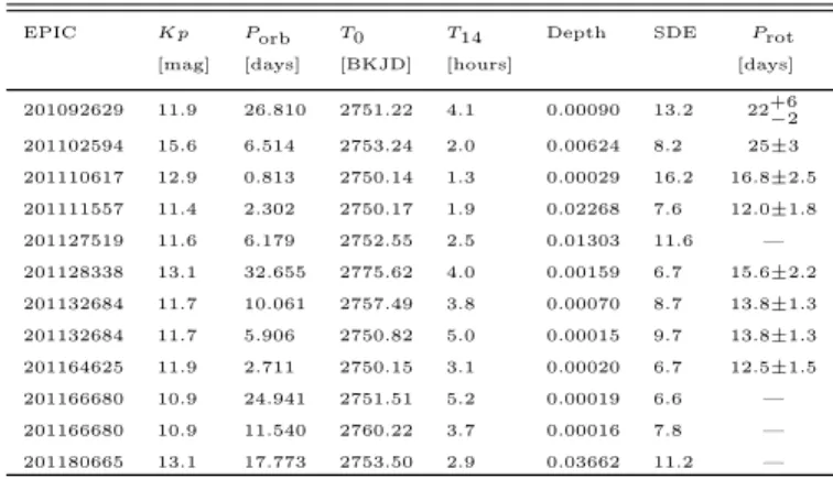
Table 1. Candidate planets detected in K2 C10. Kp denotes
magnitude in theKepler bandpass.
EPIC Kp Porb T0 T14 Depth SDE Prot
[mag] [days] [BKJD] [hours] [days]
201092629 11.9 26.810 2751.22 4.1 0.00090 13.2 22+6−2 201102594 15.6 6.514 2753.24 2.0 0.00624 8.2 25±3 201110617 12.9 0.813 2750.14 1.3 0.00029 16.2 16.8±2.5 201111557 11.4 2.302 2750.17 1.9 0.02268 7.6 12.0±1.8 201127519 11.6 6.179 2752.55 2.5 0.01303 11.6 —
201128338 13.1 32.655 2775.62 4.0 0.00159 6.7 15.6±2.2 201132684 11.7 10.061 2757.49 3.8 0.00070 8.7 13.8±1.3 201132684 11.7 5.906 2750.82 5.0 0.00015 9.7 13.8±1.3 201164625 11.9 2.711 2750.15 3.1 0.00020 6.7 12.5±1.5 201166680 10.9 24.941 2751.51 5.2 0.00019 6.6 —
201166680 10.9 11.540 2760.22 3.7 0.00016 7.8 —
201180665 13.1 17.773 2753.50 2.9 0.03662 11.2 —
Livingston et al.
Table 1(continued)
EPIC Kp Porb T0 T14 Depth SDE Prot
[mag] [days] [BKJD] [hours] [days]
201211526 11.7 21.070 2755.48 3.9 0.00030 8.3 —
201225286 11.7 12.420 2753.52 3.3 0.00065 11.6 20.8±1.6 201274010 13.9 13.008 2756.51 2.2 0.00065 7.7 —
201352100 12.8 13.383 2761.79 2.2 0.00120 12.5 36±11 201357643 12.0 11.893 2754.55 4.2 0.00107 12.3 —
201386739 14.4 5.767 2750.70 3.4 0.00134 11.1 35±6 201390048 12.0 9.455 2750.92 3.0 0.02669 7.7 —
201390927 14.2 2.638 2750.34 1.7 0.00110 12.9 —
201392505 13.4 27.463 2759.08 5.5 0.00150 9.3 —
201437844 9.2 21.057 2757.07 4.4 0.00100 10.0 —
201437844 9.2 9.560 2753.52 3.5 0.00030 9.8 —
201595106 11.7 0.877 2750.05 1.0 0.00025 9.4 —
201598502 14.3 7.515 2755.43 2.3 0.00129 7.5 —
201615463 12.0 8.527 2753.77 3.7 0.00016 7.2 —
228707509 14.8 15.351 2752.51 3.6 0.02386 13.6 —
228720681 13.8 15.782 2753.42 3.4 0.01028 14.3 9.8±1.1 228721452 11.3 4.563 2749.98 2.8 0.00020 12.6 —
228721452 11.3 0.506 2750.56 0.9 0.00010 9.6 —
228724899 13.3 5.203 2753.45 1.4 0.00113 12.3 —
228725791 14.3 6.492 2755.15 1.7 0.00110 9.8 32±3 228725791 14.3 2.251 2749.97 1.2 0.00100 7.3 32±3 228725972 12.5 4.477 2752.69 2.4 0.03270 11.5 —
228725972 12.5 10.096 2755.41 3.6 0.05928 13.0 —
228729473 11.5 16.773 2752.76 12.4 0.00199 11.6 36+5−3 228732031 11.9 0.369 2749.93 1.0 0.00040 15.1 9.4±1.9 228734900 11.5 15.872 2754.37 4.6 0.00034 8.0 —
228735255 12.5 6.569 2755.29 3.3 0.01280 12.6 31.1±2.0 228736155 12.0 3.271 2751.02 2.4 0.00027 9.3 —
228739306 13.3 7.172 2755.11 2.8 0.00070 8.1 —
228748383 12.5 12.409 2750.04 5.9 0.00024 8.0 —
228748826 13.9 4.014 2751.13 2.4 0.00102 13.2 39+6−8 228753871 13.2 18.693 2757.74 2.2 0.00082 7.7 16.4±2.3 228758778 14.8 9.301 2756.07 2.7 0.00214 7.8 —
228758948 12.9 12.203 2753.83 4.0 0.00128 12.4 11.3±1.7 228763938 12.6 13.814 2763.19 3.6 0.00036 8.8 —
228784812 12.6 4.189 2751.02 2.2 0.00014 8.9 —
228798746 12.7 2.697 2750.20 1.5 0.02587 14.1 —
228801451 11.0 8.325 2753.35 2.5 0.05325 12.9 19.5±2.7 228801451 11.0 0.584 2750.46 1.5 0.01625 10.0 19.5±2.7 228804845 12.6 2.860 2749.60 2.6 0.00020 7.3 —
228809391 12.6 19.580 2763.80 2.6 0.00100 8.3 —
228809550 14.7 4.002 2751.00 2.1 0.01259 12.5 —
228834632 14.9 11.730 2758.63 2.1 0.00111 8.6 23.6±2.1 228836835 14.9 0.728 2750.26 0.8 0.00068 15.4 —
228846243 14.5 25.554 2756.93 5.4 0.00220 10.5 —
228849382 13.8 12.120 2757.61 2.4 0.00120 7.6 —
228849382 13.8 4.097 2749.96 1.6 0.00052 8.8 —
228888935 14.1 5.691 2751.67 3.3 0.00533 10.3 7.2±1.1 228894622 13.3 1.964 2750.31 1.1 0.00183 16.3 20.8±2.4 228934525 13.4 3.676 2752.05 1.7 0.00110 14.2 28.3±3.1 228934525 13.4 7.955 2751.34 2.1 0.00110 11.4 28.3±3.1 228964773 14.9 37.209 2776.76 3.1 0.00280 6.9 —
228968232 14.7 5.520 2753.52 3.6 0.00097 8.6 —
228974324 12.9 1.606 2750.29 1.3 0.00034 13.1 22.0±2.3 228974907 9.3 20.782 2759.64 5.0 0.00010 7.2 —
229004835 10.2 16.138 2764.63 2.1 0.00036 10.6 22.2±2.5 229017395 13.2 19.099 2753.28 6.0 0.00049 8.1 —
229103251 13.7 11.667 2756.72 3.1 0.00114 9.9 —
229131722 12.5 15.480 2752.71 4.2 0.00037 8.3 —
229133720 11.5 4.037 2750.96 1.5 0.00091 12.4 11.8±1.3
2.6. Transit modeling
We used the orbital period, mid-transit time, tran-sit depth, and trantran-sit duration identified by BLS as the starting points for more detailed transit modeling. The transit light curve was generated by the Python
packagebatman (Kreidberg 2015). To reduce the data volume, we only use the light curve in a 3×T14 win-dow centered on the mid-transit times. We first tested if any of the systems showed strong transit timing variations (TTVs). We used the Python interface to the Levenberg-Marquardt non-linear least squares algo-rithm lmfit (Newville et al. 2014) to find the best-fit model of the phase-folded transit, and then fit this tem-plate to each transit separately to identify individual transit times of each candidate. Since none of the sys-tem presented in this work showed significant TTVs within the K2 C10 observations, we assumed linear ephemerides in subsequent analyses.
The transit parameters in our linear ephemeris model include the orbital periodPorb, the mid-transit timeT0, the planet-to-star radius ratioRp/R?, the scaled orbital distancea/R?, the impact parameterb≡acosi/R?, and the transformed quadratic limb-darkening coefficientsq1 andq2. Instead of fixing the parameters of the quadratic limb-darkening law to theoretical values based on stellar models, in this work we opt to allow these parameters to vary, as this allows for error propagation from stellar uncertainties. We utilize the available stellar parameters and their uncertainties to impose Gaussian priors on the limb-darkening coefficients (i.e. in the non-transformed parameter space, u1 and u2). To determine the loca-tion and width of these priors, we used a Monte Carlo method to sample the stellar parameters of each candi-date host star (Teff, logg, and [Fe/H]), and then used these to derive distributions ofu1 andu2from an inter-polated grid based on the limb-darkening coefficients for the Kepler bandpass tabulated byClaret et al. (2012). We used the median and standard deviation of these distributions to define the Gaussian limb-darkening pri-ors, and used uniform priors for all other parameters. Depending on the uncertainty in the stellar parame-ters, the limb-darkening priors determined in this way have typical widths of ∼10%, which is comparable to the uncertainty in the models used to predict them (e.g.
by a factor of 16 before averaging every 3 min window (Kipping 2010).
We adopted a Gaussian likelihood function, and found the maximum likelihood solution usingscipy.optimize
(Jones et al. 2001–present). We then sampled the joint posterior distribution using emcee (Foreman-Mackey et al. 2013), a Python implementation of the affine-invariant Markov Chain Monte Carlo ensemble sampler (Goodman & Weare 2010). We assumed the errors to be Gaussian, independent, and identically distributed, and thus described by a single parameter. In the maximum likelihood fits, we fixed the value of this parameter to the standard deviation of the out of transit flux, and during MCMC we fit for this value as a free parameter. We launched 100 walkers in the vicinity of the maxi-mum likelihood solution and ran the sampler for 5000 steps, discarding the first 1000 as “burn-in.” To ensure that the resultant marginalized posterior distributions consisted of 1000’s of independent samples (enough for negligible sampling error) we computed the autocorlation time of each parameter, and visual inspection re-vealed the posteriors to be smooth and unimodal. We summarize the transit parameter posterior distributions inTable 5using the 16th, 50th, and 84thpercentiles, and we use the posterior samples to compute other quanti-ties of interest throughout this work (i.e. Rp,Teq). The phase-folded light curves of the candidates are shown in
Figure 1, with best-fitting transit model and 1σ (68%) credible region over-plotted.
3. SPECKLE IMAGING
We observed candidate host stars with the NASA Ex-oplanet Star and Speckle Imager (NESSI) on the 3.5-m WIYN telescope at the Kitt Peak National Obser-vatory. NESSI is a new instrument that uses high-speed electron-multiplying CCDs (EMCCDs) to cap-ture sequences of 40 ms exposures simultaneously in two bands (Scott et al. (2016), Scott et al., in prep.). Data were collected following the procedures described byHowell et al.(2011). We conducted all observations in two bands simultaneously: a ‘blue’ band centered at 562nm with a width of 44nm, and a ‘red’ band cen-tered at 832nm with a width of 40nm. The pixel scales of the ‘blue’ and ‘red’ EMCCDs are 0.017564900 and 0.018188700 per pixel, respectively. We make all of our speckle imaging data publicly available via the commu-nity portal ExoFOP2. We list the individual NESSI data
products used in this work inTable 9.
Speckle imaging data were reduced following the pro-cedures described by Howell et al. (2011), resulting
2https://exofop.ipac.caltech.edu
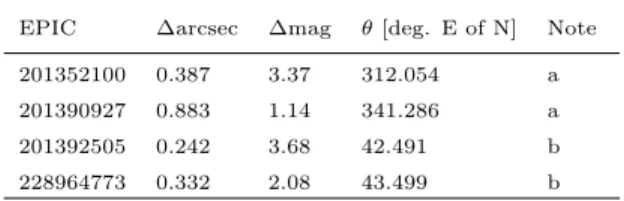
Table 2. Stars with detected companions. All de-tections made in the 832nm band.
EPIC ∆arcsec ∆mag θ[deg. E of N] Note
201352100 0.387 3.37 312.054 a 201390927 0.883 1.14 341.286 a 201392505 0.242 3.68 42.491 b 228964773 0.332 2.08 43.499 b
Note—a: The quadrant of the position angle is ambiguous, meaning it could be off by exactly 180 degrees. b: The binary model fit is of poor quality, so uncertainty may be larger than typical.
in diffraction limited 4.600×4.600 reconstructed images (256×256 pixels) of each target star. The methodol-ogy has been described in detail in previous works (e.g.
Horch et al. 2009, 2012, 2017), but we provide a brief review here for convenience.
First, the autocorrelation function of each 40 ms expo-sure is summed and Fourier transformed, resulting in the average spatial frequency power spectrum. The speckle transfer function is then deconvolved by dividing the tar-get’s power spectrum by that of the corresponding point source calibrator, yielding the square of the modulus estimate of the target’s Fourier transform. The phase information can then be recovered from bispectral anal-ysis, as first described byLohmann et al. (1983). This is accomplished by computing the Fourier transform of the summed triple correlation function of the exposures, which in combination with the modulus estimate yields the complex Fourier transform of the target. This is then filtered with a low-pass 2-d Gaussian before being inverse transformed, yielding the reconstructed image.
We extract background sensitivity limits from the re-constructed images by computing the mean and stan-dard deviation of a series of concentric annuli centered on the target star, as described byHowell et al.(2011). We then compute contrast curves by fitting a cubic spline to the kernel-smoothed 5σ sensitivity limits, ex-pressed as a magnitude difference relative to the tar-get star as a function of radius. For stars of moderate brightness (V = 10−12 mag) we typically achieve con-trasts of∼4 magnitudes at 0.200. SeeFigure 2for a plot showing all of the contrast curves obtained in this work. We detect 4 candidate host stars with secondaries, see
Table 2.
4. HIGH RESOLUTION SPECTROSCOPY
4.1. McDonald/Tull
Livingston et al.
0.2 0.0 0.2 0.9985
0.9990 0.9995 1.0000
Relative Flux
VP
201092629.01
0.1 0.0 0.1 0.995
1.000 1.005
VP
201102594.01
0.05 0.00 0.05 0.9995
1.0000 1.0005
VP
201110617.01
0.05 0.00 0.05 0.9996
0.9998 1.0000 1.0002
PC
201111557.01
0.1 0.0 0.1 0.990
0.995 1.000
PC
201127519.01
0.2 0.0 0.2 0.998
0.999 1.000
PC
201128338.01
0.2 0.0 0.2 0.9998
1.0000 1.0002
Relative Flux
VP
201132684.01
0.2 0.0 0.2 0.9995
1.0000
VP
201132684.02
0.1 0.0 0.1 0.99950
0.99975 1.00000 1.00025
PC
201164625.01
0.2 0.0 0.2 0.9998
1.0000 1.0002
VP
201166680.01
0.2 0.0 0.2 0.9998
1.0000 1.0002
VP
201166680.02
0.2 0.0 0.2 0.98
1.00
PC
201180665.01
0.2 0.0 0.2 0.9996
0.9998 1.0000
Relative Flux
VP
201211526.01
0.1 0.0 0.1 0.9995
1.0000
VP
201225286.01
0.1 0.0 0.1 0.9990
0.9995 1.0000 1.0005
PC
201274010.01
0.1 0.0 0.1 0.9990
0.9995 1.0000
PC
201352100.01
0.25 0.00 0.25 0.9990
0.9995 1.0000
VP
201357643.01
0.2 0.0 0.2 0.998
0.999 1.000 1.001
VP
201386739.01
0.1 0.0 0.1 0.99950
0.99975 1.00000 1.00025
Relative Flux
PC
201390048.01
0.05 0.00 0.05 0.999
1.000 1.001
PC
201390927.01
0.25 0.00 0.25 0.998
1.000
PC
201392505.01
0.2 0.0 0.2 0.9996
0.9998 1.0000
VP
201437844.01
0.2 0.0 0.2 0.9990
0.9995 1.0000
VP
201437844.02
0.05 0.00 0.05 0.9996
0.9998 1.0000 1.0002
PC
201595106.01
0.1 0.0 0.1 0.998
1.000 1.002
Relative Flux
VP
201598502.01
0.25 0.00 0.25 0.9998
1.0000 1.0002
VP
201615463.01
0.2 0.0 0.2 0.98
0.99 1.00
PC
228707509.01
0.2 0.0 0.2 0.990
0.995 1.000
PC
228720681.01
0.05 0.00 0.05 0.9998
1.0000 1.0002
VP
228721452.01
0.1 0.0 0.1 0.9996
0.9998 1.0000 1.0002
VP
228721452.02
0.05 0.00 0.05 0.999
1.000
Relative Flux
PC
228724899.01
0.1 0.0 0.1 0.998
0.999 1.000 1.001
VP
228725791.01
0.1 0.0 0.1 0.998
0.999 1.000 1.001
VP
228725791.02
0.1 0.0 0.1 0.9995
1.0000 1.0005
VP
228725972.01
0.2 0.0 0.2 0.9990
0.9995 1.0000 1.0005
VP
228725972.02
0.5 0.0 0.5 0.998
0.999 1.000
FP
228729473.01
0.05 0.00 0.05 0.9995
1.0000
Relative Flux
VP
228732031.01
0.25 0.00 0.25 0.99950
0.99975 1.00000 1.00025
VP
228734900.01
0.2 0.0 0.2 0.985
0.990 0.995 1.000
VP
228735255.01
0.1 0.0 0.1 0.99950
0.99975 1.00000 1.00025
VP
228736155.01
0.1 0.0 0.1 0.9990
0.9995 1.0000 1.0005
VP
228739306.01
0.25 0.00 0.25 0.9995
1.0000 1.0005
VP
228748383.01
0.1 0.0 0.1 0.999
1.000 1.001
Relative Flux
VP
228748826.01
0.1 0.0 0.1 0.9995
1.0000
PC
228753871.01
0.1 0.0 0.1 0.998
1.000 1.002
VP
228758778.01
0.2 0.0 0.2 0.999
1.000
PC
228758948.01
0.2 0.0 0.2 0.9995
1.0000
VP
228763938.01
0.05 0.00 0.05 0.99975
1.00000 1.00025 1.00050
PC
228784812.01
0.05 0.00 0.05 0.99950
0.99975 1.00000 1.00025
Relative Flux
VP
228798746.01
0.05 0.00 0.05 0.9998
1.0000
VP
228801451.01
0.1 0.0 0.1 0.99950
0.99975 1.00000
VP
228801451.02
0.1 0.0 0.1 0.9995
1.0000 1.0005
VP
228804845.01
0.1 0.0 0.1 0.9990
0.9995 1.0000
PC
228809391.01
0.1 0.0 0.1 0.985
0.990 0.995 1.000
VP
228809550.01
0.1 0.0 0.1 0.999
1.000 1.001
Relative Flux
PC
228834632.01
0.05 0.00 0.05 0.998
1.000 1.002
PC
228836835.01
0.5 0.0 0.5 0.998
1.000
PC
228846243.01
0.05 0.00 0.05 0.999
1.000
VP
228849382.01
0.1 0.0 0.1 0.999
1.000 1.001
VP
228849382.02
0.2 0.0 0.2 0.995
1.000
PC
228888935.01
0.1 0.0 0.1 0.998
0.999 1.000
Relative Flux
VP
228894622.01
0.1 0.0 0.1 0.999
1.000
VP
228934525.01
0.1 0.0 0.1 0.999
1.000
VP
228934525.02
0.2 0.0 0.2 0.996
0.998 1.000
PC
228964773.01
0.2 0.0 0.2 0.998
1.000 1.002
VP
228968232.01
0.05 0.00 0.05 0.9995
1.0000 1.0005
VP
228974324.01
0.25 0.00 0.25 Phase [days] 0.9998
0.9999 1.0000
Relative Flux
PC
228974907.01
0.1 0.0 0.1 Phase [days] 0.9996
0.9998 1.0000
PC
229004835.01
0.25 0.00 0.25 Phase [days] 0.9990
0.9995 1.0000 1.0005
VP
229017395.01
0.1 0.0 0.1 Phase [days] 0.999
1.000
PC
229103251.01
0.2 0.1 0.0 0.1 Phase [days] 0.99950
0.99975 1.00000 1.00025
VP
229131722.01
0.1 0.0 0.1 Phase [days] 0.9990
0.9995 1.0000
PC
229133720.01
Figure 1. Phase-folded transits (purple), with the best-fit transit model and 1σcredible region overplotted (orange). Candidate
0.0 0.2 0.4 0.6 0.8 1.0 1.2
Separation [arcsec]
0
2
4
6
8
m
ag
(8
32
n
m
)
WIYN/NESSI contrast curves
Detected companion
Figure 2. Contrast curves and detected companions
0.2
00201352100
0.2
00228964773
0.2
00201392505
0.4
00201390927
Figure 3. Reconstructed 832nm images of stars with de-tected companions.
echelle spectrograph (Tull et al. 1995) at the Harlan J. Smith 2.7m telescope at McDonald Observatory. Obser-vations were conducted with the 1.2×8.200 slit, yielding a resolving power ofR∼60,000. The spectra cover 375-1020 nm, with increasingly larger inter-order gaps long-ward of 570 nm. For each target star, we obtained three successive short exposures in order to allow removal of energetic particle hits on the CCD detector. We used an exposure meter to obtain an accurate flux-weighted barycentric correction and to give an exposure length that resulted in a signal/noise ratio of about 30 per pixel. Bracketing exposures of a Th-Ar hollow cathode
lamp were obtained in order to generate a wavelength calibration and to remove spectrograph drifts. This en-abled calculation of absolute radial velocities from the spectra. The raw data were processed using IRAF rou-tines to remove the bias level, inter-order scattered light, and pixel-to-pixel (“flat field”) CCD sensitivity varia-tions. We traced the apertures for each spectral order and used an optimal extraction algorithm to obtain the detected stellar flux as a function of wavelength.
We computed stellar parameters from our reconnais-sance Tull spectra usingKea(Endl & Cochran 2016). In brief, we used standard IRAF routines to perform flat fielding, bias subtraction, and order extraction, and we used a blaze function determined from high SNR flat field exposures to correct for curvature induced by the blaze. Kea uses a large grid of synthetic model stellar spectra to compute stellar effective temperatures, sur-face gravities, and metallicities. SeeTable 6for the stel-lar parameters used in this work. From a comparison with higher SNR spectra obtained with Keck/HIRES we found typical uncertainties of 100 K inTeff, 0.12 dex in [Fe/H], and 0.18 dex in logg. For a detailed description of Kea seeEndl & Cochran(2016).
4.2. NOT/FIES
We also used the FIbre-fed ´Echelle Spectrograph (FIES;Frandsen & Lindberg 1999; Telting et al. 2014) on the 2.56-m Nordic Optical Telescope (NOT) of Roque de los Muchachos Observatory (La Palma, Spain) to col-lect high-resolution (R ≈ 67 000) spectra of four C10 candidate host stars: 228729473, 228735255 (K2-140;
Giles et al.(2018), Korth et al., submitted to MNRAS), 201127519, and 228732031 (K2-131; Dai et al. 2017). The observations were carried out between February 15 to May 23, 2017 UTC, within observing programs 54-027, 55-019, and 55-202. We followed the same strategy as in Gandolfi et al. (2013) and traced the RV drift of the instrument by bracketing the science exposures with 90-sec ThAr spectra. We reduced the data us-ing standard IRAF routines and extracted the RVs via multi-order cross-correlations using different RV stan-dard stars observed with the same instrument.
4.3. TNG/HARPS-N
We observed the stars 228801451, 228732031 (K2-131;
Dai et al. 2017), 201595106, and 201437844 (HD 106315;
Livingston et al.
A34TAC 10 and A34TAC 44. We reduced the data using the dedicated off-line pipeline and extracted the RVs by cross-correlating the ´echelle spectra with a G2 numerical mask. The HARPS-N data of 228732031 have been published by our team in Dai et al. (2017). We refer the reader to that paper for a detailed description and analysis of the data. We list the results of our analysis of these spectra inTable 10.
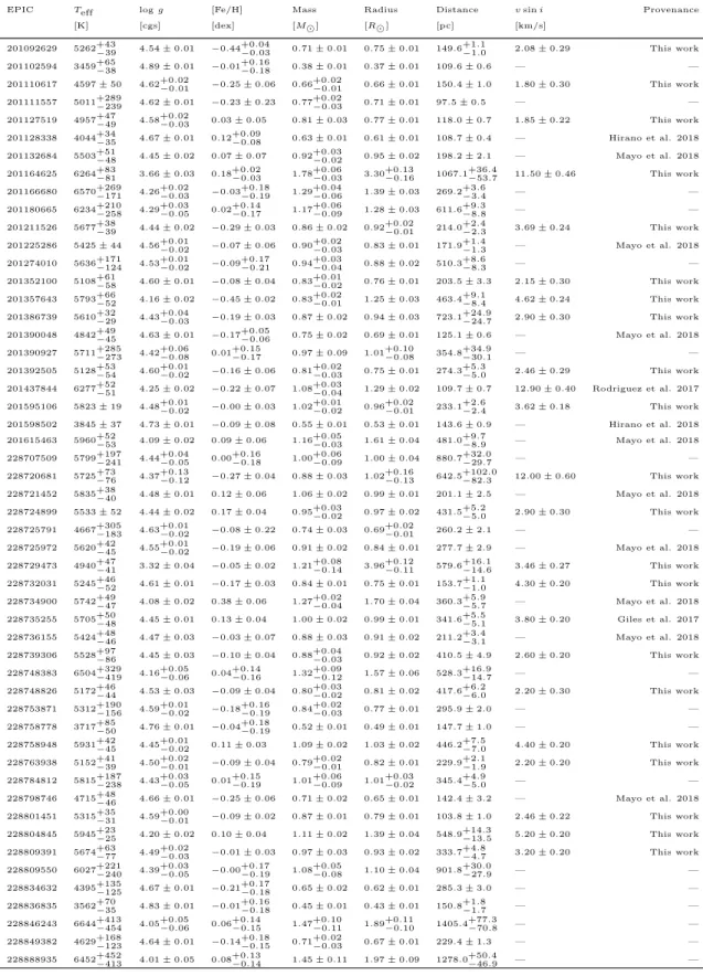
4.4. Stellar properties
We obtained spectra for 27 candidate host stars in this work, from which we derivedTeff, logg, [Fe/H], and vsini, as described in Section 4.1. We augment this set of spectroscopic stellar parameters with values from the literature for an additional 14 candidate host stars (Rodriguez et al. 2017;Hirano et al. 2018a;Mayo et al. 2018). To maximize both the quality and uniformity of the final set of stellar parameters we use in this work, we adopted the following strategy. First, we gathered 2MASSJ HKphotometry and Gaia DR2 parallaxes for all stars; 2MASS photometry is available in the EPIC, and we cross-matched to Gaia DR2 using both posi-tion and optical magnitude agreement (Kpand GaiaG band). We then used theisochrones (Morton 2015a) interface to the Dartmouth stellar model grid (Dotter et al. 2008) to estimate stellar parameters and their uncertainties using the MultiNestsampling algorithm (Feroz et al. 2013). For those stars with parameters from spectroscopic analyses, we imposed Gaussian priors on Teff, logg, and [Fe/H], with mean and standard devia-tion set by the spectroscopically derived values and their uncertainties. We also ran the same analysis without in-cluding parallax, as a check on the quality of the param-eters derived in this manner without any distance infor-mation; unsurprisingly, we found that including parallax yielded the biggest improvement for stars lacking spec-troscopy. This is perhaps most important for the M dwarfs in our sample, which suffer from systematically underestimated radii in the EPIC (see e.g.Dressing et al. 2017).
As an additional quality check, we also performed spectral analyses for the targets 201127519, 201437844, 201595106, and 228801451, using spectra from FIES and HARPS-N and SpecMatch-emp (Yee et al. 2017).
SpecMatch-emp fits the input spectra to hundreds of
library template spectra collected by the California Planet Search, and the stellar parameters (Teff, R?, and [Fe/H]) are estimated based on the interpolation of the parameters for best-matched library stars. Among them 201127519, 201595106, and 228801451 were also observed with the Tull spectrograph, and the resulting parameters by SpecMatch-empare in agreement within
∼1.5σwith those estimated from the Tull spectra by the
Keacode. For HD 106315, we obtainedTeff= 6326±110 K, R? = 1.86±0.30 R, and [Fe/H] = −0.20±0.08. WhileTeff and [Fe/H] agrees within 1σwith the litera-ture values (Rodriguez et al. 2017;Crossfield et al. 2017), R? exhibits a moderate disagreement with that in the literature (R?= 1.281+0−0..051058R Rodriguez et al. 2017). This is probably due to the small number of library stars inSpecMatch-empin the region withTeff >6300 K, but this disagreement does not have any impact on our re-sults.
5. PLANET VALIDATION
5.1. Statistical framework
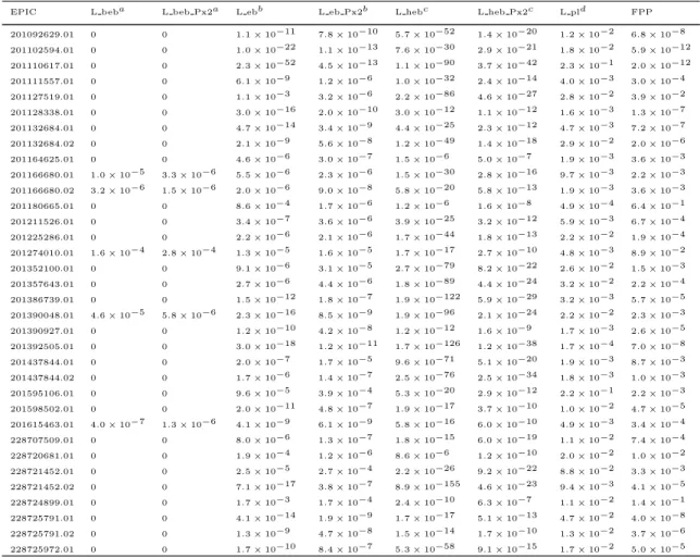
We use the open sourcevespasoftware package ( Mor-ton 2012, 2015b) to compute the false positive proba-bilities (FPPs) of each planet candidate. vespa uses
the TRILEGAL Galaxy model (Girardi et al. 2005) to
compute the posterior probabilities of both planetary and non-planetary scenarios given the observational con-straints, and considers false positive scenarios involving simple eclipsing binaries, blended background eclipsing binaries, and hierarchical triple systems. vespa models the physical properties of the host star, taking into ac-count any available broadband photometry and spectro-scopic stellar parameters, and compares a large number of simulated scenarios to the observed phase-folded light curve. Both the size of the photometric aperture and contrast curve constraints are accounted for in the cal-culations, as well as any other observational constraints such as the maximum depth of secondary eclipses al-lowed by the data. We adopt a fiducial validation cri-terion of FPP<0.01, which is reasonably conservative and also consistent with the literature (e.g.Montet et al. 2015;Crossfield et al. 2016;Morton et al. 2016). vespa
utilizes the contrast curves derived from the observa-tions listed in Table 9 and described in Section 3. To minimize the possibility of errors in the vespa calcu-lations induced by zero-point offsets or underestimated uncertainties in broadband photometry, we opt to use only the well-calibrated 2MASS J HK magnitudes and their uncertainties, taken from the EPIC, in addition to theKepler band magnitude required by vespa. The stellar parameters used as input tovespa are identical to those used in our uniform isochrones analysis (see
Section 4.4). In addition to stellar parameters, vespa
10
010
110
2P
orb[days]
10
010
1R
P[
R
]
Planets
500
750
1000
1250
1500
1750
2000
2250
T
eq[K
]
10
010
110
2P
orb[days]
10
010
1R
P[
R
]
Candidates
500
750
1000
1250
1500
1750
2000
2250
T
eq[K
]
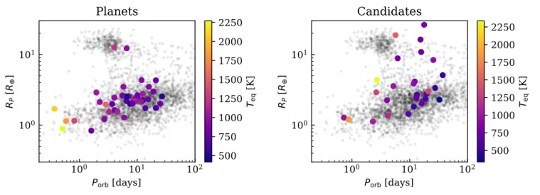
Figure 4. Validated (left) and candidate (right) planets from C10 against the background of previously confirmed or validated planets, colored by their equilibrium temperature (assuming a Bond albedo of 0.3).
Table 7. We denote final dispositions as follows: “VP” = validated planet; “PC” = planet candidate; “FP” = false positive.
All of the candidates we detect in multi-planet sys-tems meet the fiducial validation criterion of FPP < 1%. However, FPPs computed with vespa treat only the individual planet candidates in isolation, and thus do not take into account any multiplicity in each sys-tem. Stars with multiple transiting planet candidates have been shown to exhibit a lower false positive rate by an order of magnitude (Lissauer et al. 2011, 2012,
2014). For this reason we apply a “multiplicity boost” factor to the planet probability appropriate for each can-didate in a multi-planet system. Lissauer et al. (2012) estimated a multiplicity boost factor of 25 for systems containing 2 planet candidates in the Kepler field, and we apply the same factor in this work. To check that this factor is appropriate forK2 C10, we followSinukoff et al.(2016) and utilize equations (2) and (4) ofLissauer et al. (2012) to estimate the sample purity P from the integrated FPP of our sample and the number of planet candidates we detect (72). This estimate of P is quite high, perhaps due to a lack of contamination from back-ground stars due to the high galactic latitude of the field, or due to our team’s vetting procedures. The fraction of detected planet candidates in multi-systems (18/72) in conjunction with the high sample purity yields a multi-plicity boost which is significantly higher than the factor of 25 estimated by Lissauer et al.(2012) for theKepler
field. Although the true value is likely to be higher, we conservatively apply only a factor of 25, consistent with
Lissauer et al. (2012), and the FPPs inTable 5 reflect this accordingly.
5.2. Stellar companions
To ensure that the FPPs computed by vespa are re-liable, we take into account the presence of any nearby stars detected in speckle or archival imaging. Table 2
lists the nearby stars we detected via speckle imagine, along with their separations and delta-magnitudes rel-ative to the primary stars. Figure 3 shows the recon-structed speckle images for these stars, and Figure 2
shows these detections relative to the ensemble of con-trast curves from all of our speckle images. Table 3lists those stars found in the EPIC to be near and bright enough to be the source of the observed transit signals.
5.2.1. Companions detected in high resolution imaging
On the nights of 15, 17, and 2017-03-18 we acquired speckle imaging of the stars 201352100, 201390927, 201392505, and 228964773 (seeTable 9). We detected companions in the reconstructed images (see
Figure 3), so we assessed the possibility that the transit signal might not originate from the primary stars. We used the following relation between the observed transit depthδ0 and the true transit depthδin the presence of dilution from a companion ∆mmagnitudes fainter than the primary star:
δ0= δ
1 + 100.4∆m (1)
Livingston et al.
Table 3. EPIC sources within the photometric apertures which are bright enough to produce the observed transit-like signals.
EPIC Contaminant ρ[arcsec] ∆Kp[mag]
201111557 201111694 15.90 5.187 201164625 201164669 17.58 3.228 201595106 201595004 13.62 5.839 228707509 228707572 12.48 1.563 228720681 228720649 7.86 2.905 228758948 228758983 9.00 3.267
the host. For each of these four of these candidates, the secondary source is bright enough (given the observed transit depth) that we cannot rule out the possibility they are the source of the signal (seeTable 2). For this reason, we do not validate any of these candidates as planets, as we do not know the true source of the signal (and therefore the true planet size), even though they all have low FPPs.
5.2.2. Companions in the EPIC
In addition to analyzing the scenarios involving com-panions detected in high resolution speckle imaging, we also performed a search of the EPIC for any additional stars within the photometric apertures which could be the source of the observed signals. Most of these queries yielded no stars within the aperture other than the pri-mary, but there were some cases in which the query yielded a star bright enough to be the source of the observed transit signal; we list these cases in Table 3. Despite their low FPPs, we do not validate these can-didates because we do not know which star is the true host. As we expect most of these candidates to be gen-uine planets, they present good validation opportunities via higher angular resolution follow-up transit observa-tions, either from the ground or from space (i.e. with
Spitzer orCHEOPS).
5.2.3. Archival imaging
As a check on the accuracy of the sources comprising the EPIC, we also queried 1’×1’ Pan-STARRS-13 grizy
images centered at the position of each candidate host star. We found good agreement with the catalog query: nearby stars found by the catalog query were clearly visible in the images, and no nearby bright sources were
3 Data release 1, dated December 19, 2016, available at
http://ps1images.stsci.edu/cgi-bin/ps1cutouts
g
r
i
201111557
z
y
g
r
i
201164625
z
y
g
r
i
201595106
z
y
g
r
i
228707509
z
y
g
r
i
228720681
z
y
g
r
i
228758948
z
y
Figure 5. Archival grizy imaging from
Pan-STARRS-1. Shown here are candidate planet hosts with nearby
bright stars within the K2 apertures (represented by
cir-cular shaded regions). Assuming a maximum eclipse depth of 100%, the observed transit-like signal could potentially be reproduced by scenarios in which the signal is actually a faint eclipsing binary diluted by the flux from the brighter primary star. We note, however, that such scenarios would sometimes result in more “V-shaped” transits than what we observe.
seen in the images that were not previously found by the catalog query. We show these images in Figure 5, with overplotted circular regions illustrating the size and location of the apertures used to extract photometry from theK2 pixel data.
5.3. Multi-aperture light curve analysis
from “non-optimal” apertures. However, this analysis is especially important when there are widely separated neighboring stars (i.e. severalKepler pixels away) that still contribute flux to the K2 apertures, in which case it may be possible to determine the origin of the transit-like signal by this method. Based on these analyses we found that the transit signal associated with the candi-date 201164625.01 most likely originates from the neigh-boring star, 201164669 (seeTable 3and Figure 5). We also detected suspicious transit depth behavior in the light curves of 201392505.01 and 228964773.01, both of which have nearby companions detected in speckle imaging. Intriguingly, these companions are well within a Kepler pixel of the target star, so even the smallest aperture possible (oneKeplerpixel) should contain light from both the primary and secondary stars. This re-sult may indicate the presence of another (undetected) star further away, and suggests that such multi-aperture analyses should be useful for ranking the quality of can-didates when high resolution imaging is unavailable.
5.4. Transit SNR
As a final step in the validation process, we compute the transit SNR for each candidate in order to enforce a minimum transit quality standard for all planets in the validated sample. We compute the transit SNR us-ing the simple approximation that the signal scales with the transit depth and the square root of the number of transits (e.g. Bouma et al. 2017). We estimate the noise by computing the standard deviation of the out-of-transit photometry used in our light curve fits and scaling it from the K2 observing cadence to the transit duration of each candidate. We find median SNR values of 17.1 and 17.6 for the validated and candidate samples, respectively. The slightly lower SNR of the validated sample is likely attributable to the fact that candidates with higher FPPs are typically larger and have corre-spondingly deeper transits, whereas the vast majority of our validated planets are sub-Neptunes (see Figure 4). Our validated sample consists of planets with SNR > 10, with the exception of K2-254 b and K2-247 c, which have SNR values of 6.7 and 8.9, respectively. However, these are both in multi-planet systems, which increases our confidence in the veracity of the transit signals. We argue that candidates with relatively low SNR found in systems with multiple validated candidates need not be regarded with as much suspicion as similarly low SNR candidates in single-candidate systems; this is related to, but more qualitative than, the “multi-boost” argument ofLissauer et al.(2012). Indeed, many interesting plan-ets with low SNR likely remain to be found in both the
Kepler andK2 data (e.g.Shallue & Vanderburg 2018).
5.5. Pipeline comparison
To check the quality of our light curves and provide an additional layer of confidence in our candidates, we performed a parallel analysis using light curves from an independentK2 pipeline. We first downloaded the light curves ofVanderburg & Johnson(2014) from MAST for all the targets listed inTable 1, then detrended the light curves by fitting a second order polynomial to the out-of-transit data using exotrending (Barrag´an & Gandolfi 2017). To explore the transit model parameter space with MCMC, we usedpyaneti(Barrag´an et al. 2017a) to fit the detrended light curves with uniform priors for all parameters; more description of thepyanetiMCMC evolution and parameter estimation can be found in Bar-rag´an et al. (2017b) and Gandolfi et al. (2017). For the majority of candidates, the main transit parame-ters of interest (Porb, Rp/R?, b, and a/R?) are consis-tent within 1σ between our two independent analyses, although there are some cases in which marginally sig-nificant differences were found. These differences are likely to be the result of different handling of the K2
systematics and/or the stellar variability in the light curves. The overall good agreement between these two independently-derived sets of transit parameters pro-vides an additional layer of confidence in the quality of the candidates. The results of this comparison are listed inTable 12.
6. DISCUSSION
6.1. Validated planets
We validate 44 planets out of our sample of 72 can-didates, and tabulate the FPPs along with parameter estimates of interest in Table 5. Of the 44 validated planets we report here, 20 of them have been previ-ously statistically validated or confirmed: 201598502.01, 228934525.01, and 228934525.02 (K2-153 b, K2-154 bc;
Hirano et al. 2018a); 228735255.01 (K2-140 b; Giles et al. (2018), Korth et al., submitted to MNRAS); 201437844.01 and 201437844.02 (HD 106315 bc; Cross-field et al. 2017; Rodriguez et al. 2017); 228732031.01 (K2-131 b;Dai et al. 2017); and 13 others were recently validated byMayo et al.(2018). In the left panel of Fig-ure 4 we plot the planetary radii, orbital periods, and equilibrium temperatures of the validated planets in the sample.
We investigated the impact of these new planets to the population of currently known planets by querying the NASA Exoplanet Archive4(Akeson et al. 2013). We
computed the fractional enhancement to the known
Livingston et al.
8
10
12
14
J [mag]
0.5
1
2
4
8
16
R
P
[
R
]
3%
4%
6%
17%
5%
1%
11%
3%
1%
1%
C10 Enhancement
0
2
4
6
8
10
12
14
16
Enhancement [%]
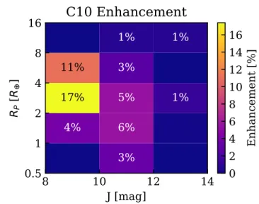
Figure 6. The fractional enhancement to the population of previously validated or confirmed planets from our sample of 44 validated C10 planets.
ulation due to the 44 planets as a function of planet size and host star brightness (seeFigure 6). As of June 12, 2018, the populations of super-Earths (Rp ≈ 1–2R⊕), sub-Neptunes (Rp ≈ 2–4R⊕), and sub-Saturns (Rp ≈ 4–8R⊕) orbiting bright stars (J = 8–10 mag) are en-hanced by ∼4%, ∼17%, and ∼11%, respectively. Be-cause of the brightness of the host stars, many of these planets are ideal for detailed characterization studies via precision Doppler and transmission spectroscopy, which we discuss in greater detail inSection 6.4.
6.2. Candidates
Out of the 72 planet candidates we present here, 27 are not validated. Most cannot be validated due to the FPP being above our fiducial validation criterion of 1% or the presence of a contaminating star within the photometric aperture. SeeTable 7for the likelihoods of various false positive scenarios and the planet scenario, as computed
by vespa. There are several candidates which we do
not validate for other reasons, which we discuss below. In the right panel of Figure 4 we plot the planetary radii, orbital periods, and equilibrium temperatures of the non-validated candidates.
The candidate 228729473.01 exhibits a long tran-sit duration, and subsequent spectroscopic analyses re-vealed large RV variations which are consistent with the candidate being a false positive involving an M dwarf eclipsing a sub-giant, see Csizmadia et al (in prep.) for more details. The light curve of 229133720.01 ex-hibits low levels of variability in phase with the tran-sit signal, which could be due to ellipsoidal variations; thus we do not validate the candidate in spite of its
low FPP. Although 201390048.01 was recently validated (K2-162 b; Mayo et al. 2018), we found marginal ev-idence of odd-even variations in the light curve of this candidate, which could be an indication that the signal is actually caused by an eclipsing binary at twice the esti-mated orbital period. Althoughvespaaccounts for this scenario in its FPP calculation, we do not validate the candidate even though its FPP is below 1%. The can-didate 201180665.01 has a relatively high FPP (∼64%), and also a suspiciously large radius estimate (∼26R⊕). Although spectroscopic characterization could yield a different radius estimate for the host star (and thus also for the candidate), we conclude that this is most likely an eclipsing M dwarf companion. The candidates 228974907.01, and 228846243.01 do not have particu-larly low FPPs, but they may be interesting targets for further observations due to their relatively long orbital periods. The candidate 201128338.01 was statistically validated previously in the literature (K2-152 b;Hirano et al. 2018a); we find a similarly low FPP, but we do not validate it simply because it has fewer than three transits in theK2 photometry (and thus odd/even vari-ations in transit depth cannot be robustly ruled out). Further observations will shed light on the true na-ture of these candidates, either by measuring RV vari-ations with precision spectrographs or via simultaneous multi-band transit observations with instruments such as MuSCAT (Narita et al. 2015) and MuSCAT2 (agriz
clone of MuSCAT now in operation at Teide Observa-tory).
The integrated FPP is ∼2.1 for the full set of 72 candidates, which implies the existence of two false positives in the sample. We have already confirmed that 228729473.01 is a false positive via RV observa-tions (see Csizmadia et al., in prep.), and we suspect 229133720.01, 201390048.01, and 201180665.01 of being false positives, as described above. Therefore, we expect no false positives among the remainder of the sample, and most of the 27 unvalidated candidates could be sta-tistically validated or confirmed by future observations.
6.3. Interesting new systems
6.3.1. Ultra-short period planets
2017b; Malavolta et al. 2018). The radii of these USPs place all three of them below the recently observed gap in the radius distribution (Fulton et al. 2017;Van Eylen et al. 2017) which was predicted as a consequence of pho-toevaporation (e.g.Owen & Wu 2013;Lopez & Fortney 2014). These three USPs are therefore likely to be rocky and have high densities, consistent with having lost any primordial or secondary atmospheres they might once have had. Of these validated USPs, we measured the metallicity of the host stars spectroscopically for three of them; K2-229 appears to have only a modestly sub-solar metallicity of−0.09±0.02 [Fe/H], but K2-131 and K2-156 have more significantly sub-solar metallicities of −0.17±0.03 and−0.25±0.06 [Fe/H], respectively (see
Table 6). Due to their small size, these USPs are likely to have a mass less than 5–6M⊕, and thus the sub-solar metallicity of their host stars would be consistent with the USP mass-metallicity trend noted bySinukoff et al.
(2017) (i.e. similar to Kepler-78 b and Kepler-10 b). The G dwarf K2-223 and K dwarf K2-229 are both relatively bright (Kp ∼ 11 mag), and host planets with predicted masses and Doppler semi-amplitudes well within the reach of current precision spectrographs, such as HARPS or HIRES. K2-156 b orbits a slightly fainter star and has a slightly smaller predicted mass and Doppler semi-amplitude, but is also a viable target for characterization with today’s instrumentation. Such mass measurements would yield densities and constrain the bulk compositions of these USPs, which would en-able tests of USP formation theories.
In addition to the four validated USPs mentioned above, we also note that our sample contains two USP candidates: 201595106.01 and 228836835.01. We do not validate 201595106.01 because of the presence of a faint star in the EPIC with a ∆Kpof 5.839 and a separation of 13.6200(see Table 3), which is within the photomet-ric aperture we used to extract theK2 light curve. We do not validate 228836835.01 because it has a FPP of ∼4% and thus does not meet our validation criterion. Future observations could potentially rule out false pos-itive scenarios for both of these candidates, resulting in the validation of two more USPs fromK2 C10.
6.3.2. Multi-planet systems
Of the 44 validated planets in our sample, 18 of them were found in two-planet systems, which enables the study of their orbital architectures and evolution. Four of these systems have orbital architectures with period ratios just wide of a 2:1 commensurability, and two are close to a 3:1 commensurability. The pairs closest to 2:1 are K2-243 bc and K2-154 bc, which both have Pc/Pb ≈ 2.16. The relatively large fraction of
multi-planet systems (4/9) in our sample with period ratios just wide of a 2:1 commensurability is reminiscent of the distribution of orbital architectures observed with Ke-pler (Fabrycky et al. 2014). K2-254 bc and K2-247 bc are both just inside a 3:1 commensurability, with period ratios ofPc/Pb ≈2.96 and Pc/Pb ≈2.89, respectively. Although we did not detect any significant TTVs in the
K2 data, some of these systems may have TTVs which could be detected with higher cadence transit observa-tions.
Intriguingly, two of the four validated USPs in the sample were found in two-planet systems with large pe-riod ratios, similar to the Kepler-10 system: K2-223 bc has Pc/Pb ≈ 9.02, and K2-229 bc has Pc/Pb ≈ 14.25. The presence of an additional transiting planet decreases the likelihood that these USPs reached their current or-bits via dynamical scattering, as this would increase the chances of higher mutual inclinations; even after tidal circularization, the geometric transit probability would be decreased by a higher likelihood of non-coplanarity. This is consistent with previous analyses in which USP systems have been noted to be dynamically cold (e.g.
Dai et al. 2017).
6.4. Characterization targets
We predicted the masses of the candidates using the probabilistic mass-radius relation of Wolfgang et al.
(2016)5 (see Table 5). The predicted masses enabled
us to compute other quantities of interest, which we then used to identify potentially interesting targets for follow-up characterization via Doppler and transmission spectroscopy.
6.4.1. Doppler targets
We computed the expected Doppler semi-amplitude due to the reflex motion of the host star induced by each planet (seeTable 5). We used these expected semi-amplitudes in conjunction with the brightness of the host stars to identify planets in the sample which are good targets for radial velocity (RV) follow-up study us-ing current and future facilities. Such RV observations will reveal the planets’ densities and constrain their bulk compositions. This is of particular interest for relatively small planets with radii in the range 1.5−2.5 R⊕ be-cause such measurements could enable tests of planet formation theories and post-processes, such as the pho-toevaporation (e.g.Owen & Wu 2013;Lopez & Fortney 2014), which has been proposed to explain the observed gap in the radius distribution (Fulton et al. 2017; Van Eylen et al. 2017). However, because of the difficulty of
Livingston et al.
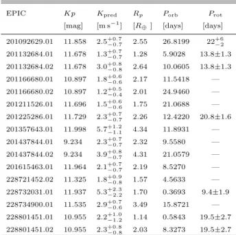
detecting the small Doppler signals of such planets, it is especially important to identify such planets which are orbiting relatively bright stars, for which the RV preci-sion required to measure their masses is more readily ob-tainable. Table 4lists validated planets with predicted Doppler semi-amplitudes greater than 1 m s−1 orbiting stars brighter than Kp = 12 mag. For convenience, we also list planetary orbital periods and stellar rota-tional periods (when available); potentially confounding quasi-periodic RV signals produced by stellar magnetic activity are less likely to present a challenge for mass measurement when the orbital period is far from the stellar rotational period (or a harmonic). We note that 228732031.01 (K2-131 b) and 228801451.01 (K2-229 b) both already have measured masses via precision RVs (Dai et al. 2017;Santerne et al. 2018).
Another possibly interesting RV target is K2-257 b, a sub-Earth-size planet orbiting a nearby M dwarf. Al-though the planet’s radius is only 0.83+0−0..0605 R⊕, the Doppler semi-amplitude could be as high as ∼1 m s−1 due to the low mass of the host star and the planet’s short orbital period. The host star is moderately bright (Kp= 12.873,J = 10.477 mag), so this presents an op-portunity to directly measure the mass of a sub-Earth with one of today’s high precision optical or NIR spec-trographs. Such a measurement would yield the planet’s density and constrain its composition, as well as improve our knowledge of the mass-radius relation for small plan-ets. The only other sub-Earth-size planet known to tran-sit a similarly bright M dwarf is Kepler-138 b, for which the mass has been measured only via transit timing vari-ations (Jontof-Hutter et al. 2015;Almenara et al. 2018).
6.4.2. Atmospheric targets
In order to identify viable new targets for atmospheric studies via transmission spectroscopy, we used the prop-erties of the host stars and planets to predict atmo-spheric scale heights and the amplitudes of the wave-length dependence of transit depth (δTS). Following
Miller-Ricci et al.(2009), we calculated the atmospheric scale heightH andδTS for each validated planet by
H= 29.26 (µ/28.96)
Teq
g [m] (2)
δTS∼10H·Rp/R2?, (3)
where µ, Teq, and g are the mean molecular weight, planet equilibrium temperature, and planet surface gravity, respectively. We used the predicted planet mass estimated in Section 6.4 to predict the surface gravity, and assumed a bond albedo of 0.3 and a mean molecu-lar weight µ= 2 (hydrogen-dominated atmosphere) for each planet (see Table 11). We note that this assump-tion forµis likely to be invalid for the smaller planets in
Table 4. Validated planets with predicted Doppler
semi-amplitudes greater than 1 m s−1 orbiting stars brighter
thanKp= 12 mag. Note: 228721452.01 is not listed here
because it doesn’t meet these criteria, but RV measure-ments to constrain the mass of 228721452.02 could also reveal the inner planet’s mass, as both Keplerian signals would need to be accounted for in the RV analysis.
EPIC Kp Kpred Rp Porb Prot
[mag] [m s−1] [R
⊕] [days] [days]
201092629.01 11.858 2.5−+00..77 2.55 26.8199 22+6−2 201132684.01 11.678 1.3+0−0..77 1.28 5.9028 13.8±1.3 201132684.02 11.678 3.0+0−0..88 2.64 10.0605 13.8±1.3 201166680.01 10.897 1.8+0.6
−0.6 2.17 11.5418 —
201166680.02 10.897 1.2+0−0..54 2.01 24.9460 — 201211526.01 11.696 1.5+0−0..66 1.75 21.0688 — 201225286.01 11.729 2.3+0.7
−0.7 2.26 12.4220 20.8±1.6
201357643.01 11.998 5.7+1−1..21 4.34 11.8931 — 201437844.01 9.234 2.3+0−0..77 2.32 9.5580 — 201437844.02 9.234 3.9+0−0..87 4.31 21.0579 — 201615463.01 11.964 2.1+0.7
−0.7 2.19 8.5270 —
228721452.02 11.325 1.8+0−0..98 1.57 4.5633 — 228732031.01 11.937 5.3+2−2..32 1.70 0.3693 9.4±1.9 228734900.01 11.535 2.9+0.7
−0.6 3.49 15.8721 —
228801451.01 10.955 2.2+1−1..02 1.14 0.5843 19.5±2.7 228801451.02 10.955 2.3+0−0..88 2.03 8.3273 19.5±2.7
our sample (i.e. Rp .1.5–2R⊕), as they are not likely to have substantial hydrogen-dominated atmospheres; these smaller planets likely have higher mean molecular weight atmospheres, which would make their character-ization via transmission spectroscopy more challenging. The validated planets K2-140 b and K2-255 b both orbit relatively bright host stars (J <12 mag) and have large expected transmission spectroscopy signals (δTS >200 ppm), and thus could be interesting targets for future atmospheric characterization.
7. SUMMARY
plan-ets, which could potentially be validated via further ob-servations and analysis.
This work was carried out as part of the KESPRINT consortium. The WIYN/NESSI observations were con-ducted as part of an approved NOAO observing pro-gram (P.I. Livingston, proposal ID 2017A-0377). Data presented herein were obtained at the WIYN Observa-tory from telescope time allocated to NN-EXPLORE through the scientific partnership of the National Aero-nautics and Space Administration, the National Sci-ence Foundation, and the National Optical Astronomy Observatory. This work was supported by a NASA WIYN PI Data Award, administered by the NASA Ex-oplanet Science Institute. NESSI was funded by the NASA Exoplanet Exploration Program and the NASA Ames Research Center. NESSI was built at the Ames Research Center by Steve B. Howell, Nic Scott, El-liott P. Horch, and Emmett Quigley. The authors are
honored to be permitted to conduct observations on Iolkam Du’ag (Kitt Peak), a mountain within the To-hono O’odham Nation with particular significance to the Tohono O’odham people. J. H. L. gratefully ac-knowledges the support of the Japan Society for the Promotion of Science (JSPS) Research Fellowship for Young Scientists. This work was supported by Japan Society for Promotion of Science (JSPS) KAKENHI Grant Number JP16K17660. M.E. and W.D.C. were supported by NASA grant NNX16AJ11G to The Uni-versity of Texas. This paper includes data collected by theKepler mission. Funding for theKepler mission is provided by the NASA Science Mission directorate.
Facilities:
Kepler, WIYN (NESSI), McDonald(Tull), NOT (FIES), TNG (HARPS-N)
Software:
scipy, emcee, batman, vespa, IRAF,pyaneti,exotrending
REFERENCES
Adams, E. R., Jackson, B., Endl, M., et al. 2017, AJ, 153, 82
Akeson, R. L., Chen, X., Ciardi, D., et al. 2013, PASP, 125, 989
Almenara, J. M., D´ıaz, R. F., Dorn, C., Bonfils, X., & Udry, S. 2018, MNRAS, 478, 460
Barrag´an, O., & Gandolfi, D. 2017, Exotrending: Fast and
easy-to-use light curve detrending software for
exoplanets, Astrophysics Source Code Library, , , ascl:1706.001
Barrag´an, O., Gandolfi, D., & Antoniciello, G. 2017a,
pyaneti: Multi-planet radial velocity and transit fitting,
Astrophysics Source Code Library, , , ascl:1707.003
Barrag´an, O., Gandolfi, D., Dai, F., et al. 2017b, ArXiv
e-prints, arXiv:1711.02097
Bouma, L. G., Winn, J. N., Kosiarek, J., & McCullough, P. R. 2017, ArXiv e-prints, arXiv:1705.08891
Cabrera, J., Csizmadia, S., Erikson, A., Rauer, H., & Kirste, S. 2012, A&A, 548, A44
Cabrera, J., Barros, S. C. C., Armstrong, D., et al. 2017, A&A, 606, A75
Christiansen, J. L., Vanderburg, A., Burt, J., et al. 2017, AJ, 154, 122
Ciardi, D. R., Crossfield, I. J. M., Feinstein, A. D., et al. 2018, AJ, 155, 10
Claret, A., Hauschildt, P. H., & Witte, S. 2012, VizieR Online Data Catalog, 354
Cosentino, R., Lovis, C., Pepe, F., et al. 2012, in Proc. SPIE, Vol. 8446, Ground-based and Airborne Instrumentation for Astronomy IV, 84461V
Crossfield, I. J. M., Petigura, E., Schlieder, J. E., et al. 2015, ApJ, 804, 10
Crossfield, I. J. M., Ciardi, D. R., Petigura, E. A., et al. 2016, ApJS, 226, 7
Crossfield, I. J. M., Ciardi, D. R., Isaacson, H., et al. 2017, AJ, 153, 255
Csizmadia, S., Pasternacki, T., Dreyer, C., et al. 2013, A&A, 549, A9
Dai, F., Winn, J. N., Gandolfi, D., et al. 2017, AJ, 154, 226 David, T. J., Hillenbrand, L. A., Petigura, E. A., et al.
2016a, Nature, 534, 658
David, T. J., Conroy, K. E., Hillenbrand, L. A., et al. 2016b, AJ, 151, 112
Dotter, A., Chaboyer, B., Jevremovi´c, D., et al. 2008,
ApJS, 178, 89
Dressing, C. D., Vanderburg, A., Schlieder, J. E., et al. 2017, AJ, 154, 207
Endl, M., & Cochran, W. D. 2016, PASP, 128, 094502 Fabrycky, D. C., Lissauer, J. J., Ragozzine, D., et al. 2014,
ApJ, 790, 146
Feroz, F., Hobson, M. P., Cameron, E., & Pettitt, A. N. 2013, ArXiv e-prints, arXiv:1306.2144
Foreman-Mackey, D., Hogg, D. W., Lang, D., & Goodman, J. 2013, PASP, 125, 306