SOME CONTRIBUTIONS TO HIGH DIMENSIONAL STATISTICAL
LEARNING
Hanwen Huang
A dissertation submitted to the faculty of the University of North Carolina at Chapel Hill in partial fulfillment of the requirements for the degree of Doctor of Philosophy in the Department of Statistics and Operations Research (Statistics).
Chapel Hill 2011
Approved by
ABSTRACT
HANWEN HUANG: Some Contributions to High Dimensional Statistical Learning (Under the direction of Professor J. S. Marron and Professor Yufeng Liu)
This dissertation consists of two major contributions to high dimensional statistical learn-ing. The focus is on classification which is one of the central research topics in the field of statistical learning. This research is on both binary and multiclass learning.
For binary classification, we propose the Bi-Directional Discrimination (BDD) method which generalizes linear classifiers from one hyperplane to two or more hyperplanes. BDD combines the strengths of linear and general nonlinear methods. Linear classifiers are very popular, but can suffer some serious limitations when the classes have distinct sub-populations. General nonlinear classifiers can give improved classification error rates, but do not give clear interpretation of the results and present great challenges in terms of overfitting in high dimensions. BDD gives much of the flexibility of a general nonlinear classifier while maintaining the interpretability, and less tendency towards overfitting, of linear classifiers. While the idea is generally applicable, we focus our discussion on the gen-eralization of the Support Vector Machine (SVM) and Distance Weighted Discrimination (DWD) methods. The performance and usefulness of the proposed method are assessed using asymptotics, and demonstrated through analysis of simulated and real data.
For multiclass learning, the DWD method is generalized from the binary case to the multiclass case. DWD is a powerful tool for solving binary classification problems which has been shown to improve upon SVM in high dimensional situations. We extend the binary DWD to the multiclass DWD. In addition to some well known extensions which simply combine several binary DWD classifiers, we propose a global multiclass DWD (MDWD) which finds a single classifier that simultaneously considers all classes. Our theoretical
Table of Contents
List of Tables . . . vii
List of Figures . . . viii
1 Introduction 1 1.1 Statistical Classification Problem . . . 1
1.2 Summary of Existing Classification Methods . . . 3
1.3 Kernel Space . . . 10
1.4 Bi-Directional Discrimination . . . 14
1.5 Multiclass Classification . . . 16
2 Bi-Directional Discrimination with Application to Data Visualization 19 2.1 Introduction . . . 19
2.2 Bi-Directional Discrimination Framework . . . 23
2.2.1 Review of Uni-Directional Methods . . . 23
2.2.2 Bi-Directional Discrimination . . . 25
2.2.3 Starting Points . . . 27
2.2.4 More Than Two Directions . . . 33
2.3 Visualization, Simulation and Data Analysis . . . 34
2.3.1 Simulated Low Dimensional Examples . . . 35
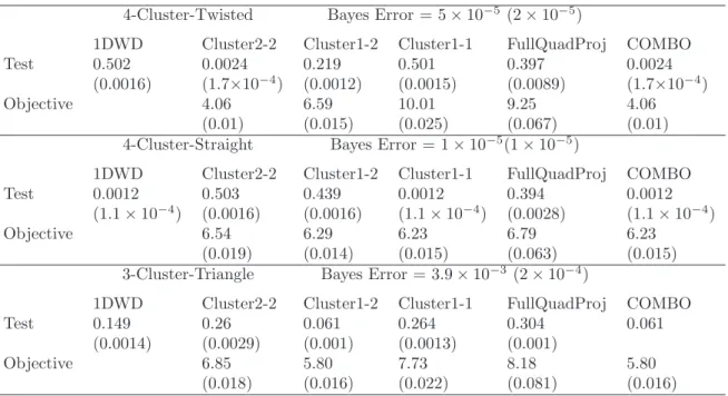
2.3.2 Simulated High Dimensional Examples . . . 39
2.3.3 Simulated Tri-Directional Examples . . . 44
2.3.4 Real Data . . . 46
2.4 Mathematical Statistics . . . 51
2.4.1 Four Clusters Case . . . 52
2.4.2 Three Clusters Case . . . 58
2.5 Proof . . . 59
2.5.1 Proof of Theorems 2.1 and 2.2 . . . 59
2.5.2 Proof of Theorem 2.3 . . . 63
2.6 Discussion . . . 68
3 Multiclass Distance Weighted Discrimination 70 3.1 Introduction . . . 70
3.2 Illustration of Batch Adjustment . . . 73
3.3 Methodology . . . 77
3.3.1 Simple Pair-Wise Extension . . . 77
3.3.2 Full Multiclass Version . . . 79
3.4 Theoretical Properties . . . 80
3.4.1 Fisher Consistency of Pair-Wise Version . . . 81
3.4.2 Fisher Consistency of Full Multiclass Version . . . 82
3.5 Simulations . . . 84
3.6 Proof . . . 88
3.6.1 Proof of Theorem 3.1 . . . 88
3.6.2 Proof of Theorem 3.2 . . . 88
List of Tables
2.1 Performance summary, average error rates over 100 simulations, of the application of the one-direction and the two-direction classification methods to three two-dimensional simulation
ex-amples. The numbers in the parentheses show standard errors. . . 38 2.2 Performance summary, average error rates over 100 simulations,
of the application of the one-direction and the two-direction classification methods to three high-dimensional simulation
ex-amples. The numbers in the parentheses show standard error. . . 44 2.3 Cross validation errors over 100 replications for the human lung
carcinoma microarray data set. The numbers in the parentheses
show standard errors. . . 49 2.4 Cross validation errors for GBM data MES versus NL . . . 50
3.1 Test errors (in percentage) over 100 replications . . . 86
List of Figures
1.1 Illustration of SVM using a toy example. The red plus signs represent the positive class and the blue circle signs represent the negative class. The black boxes highlight the support vec-tors. The black dashed lines show where the functional margin
is 1. . . 8 1.2 Illustration of the kernel embedding idea using a two-dimensional
toy example. The four panels use different polynomial embed-ding. The white band represents the decision boundary. The two classes are represented by red plus and blue circle sym-bols. Results shown in the four panels are obtained by using variables x1, x2 (upper-left), x1, x2, x21 (upper-right), x1, x2, x22
(lower-left), and x1, x2, x21, x22 (lower-right), respectively. . . 11
2.1 Toy data example in two dimensions with three different dis-crimination curves shown using a solid line-type. Red color (plus and “x” symbols’) indicates the positive class and blue color (up and down triangles) indicates the negative class. Dif-ferent symbols in the same class represent difDif-ferent sub-clusters. Note the two non-linear methods give (middle and right panels)
major improvements. . . 20 2.2 Illustration plots for both one-direction SVM (left panel) and
two-direction SVM (right panel). Solid lines represent decision boundaries. Dashed and dotted lines in the left panel are de-fined by f = 1 and f = −1 respectively. Dashed curves and Dotted curves in the right panel are defined by f1f2 = 1 and
f1f2 =−1 respectively. . . 26
2.3 KDE plot of objective function values for different starting points. . . 29 2.4 Illustration of some different sub-cluster situations for binary
classification problems. Red color (plus and “x” symbols’) in-dicates the positive class and blue color (up and down triangles) indicates the negative class. Different symbols in the same class
2.5 Application to 4-Cluster-Twisted type of two-dimensional sim-ulated data set. This realization was carefully chosen to show both types of local optima (left panel) and the global optimum (central panel). Observed objective values and their relative frequencies based on 1000 random starts are shown in the table
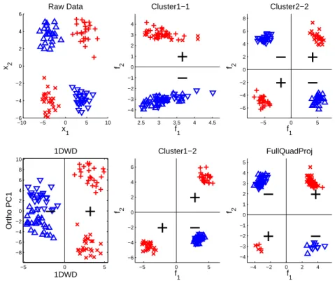
(right panel). . . 37 2.6 Application to 4-Cluster-Twisted type of high dimensional
sim-ulated data set. Upper left panel shows the raw data projected onto the first two directions. Projections onto 1DWD and or-thogonal PC1 directions are shown in the lower left panel. Pro-jections ontof1,f2 directions are shown in the middle and right
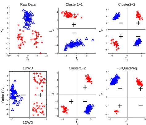
panels. . . 40 2.7 Application to 3-Cluster-Triangle type of high dimensional
sim-ulated data set. Upper left panel shows the raw data projected onto the first two directions. Projections onto 1DWD and or-thogonal PC1 directions are shown in the lower left panel. Pro-jections ontof1,f2 directions are shown in the middle and right
panels. . . 41 2.8 Visualization of a 4-Cluster-Straight example using Cluster1-1
initialization for both training (left) and test (right) data. . . 45 2.9 Classification results for the Linear 4-Cluster Gaussian mixture
example: The positive class is a mixture of N(−7.5,1) and N(2.5,1) denoted by ”+” and ”x” symbols respectively and the negative class is a mixture ofN(−2.5,1) and N(7.5,1) de-noted by triangles. The left panel is the classification boundary obtained by 1SVM; the middle panel shows the classification boundary obtained by BDD; the right panel shows the clas-sification boundary obtained by TDD. The error rates show that the one-directional method and BDD deliver similar
per-formance while TDD works the best for this example. . . 45 2.10 Classification results for the donut example. The positive class,
denoted by ”+” symbol, lies within a small center, the negative class, denoted by triangle, surrounds this entirely. The top left, top right, bottom left, bottom right display the classification boundaries by 1SVM, BDD, TDD, and the full quadratic-kernel SVM, respectively. Note that BDD offers improvement over the one-directional method (the error rate changes from 31% to 15%), and TDD further improves BDD(error rate changes from 15% to 5%). Interestingly, TDD gives performance that is not far from that of the full quadratic-kernel SVM although
it only uses three directions. . . 46
2.11 Application to the human lung carcinoma microarray data set: Normal (red ”+”) + SmallCell (red ”x”) versus Carcinoid (blue up-triangle) + Colon (blue down-triangle). Note Cluster2-2
method correctly subdivide the classes. . . 48 2.12 Application to GBM data set: MES (red ”+” sign) versus NL
(blue triangle). . . 50 2.13 Heatmap of GBM data by using top 200 genes selected from
1DWD methods (left panel) and BDD Cluster1-2 methods (right
panel). Genes are in the rows and samples are in the columns . . . 51 2.14 Illustration of the mean positions (C+1,d,C+2,d,C−1,d,C−2,d) of
the four clusters, where (C+1,d,C+2,d) belong to the positive
class and (C−1,d,C−2,d) belong to the negative class. . . 55
2.15 Summary of the classification performance given in Theorem
2.2 for the one-direction methods and the two-direction methods. . . 57
3.1 PCA projection scatter plot view of raw GBM data, showing 1D (diagonal) and 2D projections of raw data onto PC direc-tions. Groupings of colors indicate batch biases. Samples from Classical, Mesenchymal, Proneural, and Neural are indicated by “+”, “x”, circle and triangle symbols respectively. This shows a very strong batch effect, so that adjustment is essential before
combining data sets. . . 75 3.2 PCA scatter plot view of MDWD adjusted GBM data (labels
are the same as in Figure 3.1), showing effective removal of
batch biases. Biological class differences are now much more clear. . . 76 3.3 Plots of data points and decision boundaries in the first two
coordinate axis directions for one training set of Example 2. Upper left panel for Bayes boundary, upper right for MDWD, lower left for OVR, lower right for OVO. The numbers in the
CHAPTER 1
Introduction
Statistical learning plays a key role in many areas of science, finance and industry. The major focus of statistical learning research is to automatically learn to recognize complex patterns and make intelligent decisions based on data (Duda et al. (2000); Hastie et al. (2009)). This learning process falls into two main categories: supervised learning, and unsupervised learning. In supervised learning, the training sample data comprise input vectors along with the corresponding target values (output objects). The task of the supervised learner is to find a model (hypothesis) using the given data and to predict the target values for any new data. Supervised learning is called classification if the target values can be categorized into discrete classes. Unsupervised learning is a class of problems in which one seeks to summarize and explain key features of the data. It is distinguished from supervised learning in that the given data consists of input vectors without any corresponding target values. Our work focuses on classifications.
1.1
Statistical Classification Problem
input for the ith training case, and let yi be the corresponding class label which can only
take values in a discrete set. Classification is the problem of building a classification rule ˆ
y = ˆG(x) based on the training sample (x1, y1),· · · ,(xn, yn) of labeled cases, where the
joint values of all of the variables are known. This rule will enable us to predict the class label ˆy for any new object with input x.
The simplest and most widely studied case is two-class learning where there are only two classes or categories. The two classes are often coded as −1 and +1. The more complicated case is calledmulti-class learning when there are more than two classes. The most commonly used coding forK-classes is an element ofG ={1,· · · , K}.
Suppose that (x, y) are random variables governed by some joint probability distribution P(x, y), and the examples are independently and identically generated from P(x, y). The classification can be formally characterized as a density estimation problem where one is concerned with determining properties of the conditional probability P(y|x). Once the conditional (discrete) distribution P(y|x) is given, theBayes classif ierclassifies the object to the most probable class, i.e., ˆG(x) = gk if P(gk|x) = maxg∈GP(g|x).
1.2
Summary of Existing Classification Methods
There are many existing classification methods in the literature. Examples include K-Nearest Neighbors (kNN) (Cover and Hart (1967)), Neural Networks (see Anderson and Rosenfeld (1988) for a good discussion), Fisher Linear Discrimination Analysis (LDA) (Fisher (1936)), Logistic Regression (see Section 4.4 in Hastie et al. (2009) for a good discussion), Support Vector Machine (SVM) (proposed by Vapnik (1995), see Cristianini and Taylor (2000) for a good introduction) and Distance Weighted Discrimination (DWD) (Marron et al. (2007)). In the following, we give a brief description of each method for the binary classification problem.
K-nearest Neighbors
The k-nearest neighbors (kNN) algorithm is amongst the simplest of all machine learn-ing methods. In this method, one first finds in the d-dimensional feature space the k closest objects from the training set to the new object being classified. The object is simply assigned to the majority class amongst these k neighbors, where k is a positive integer, typically small. If k = 1, then the object is simply assigned to the class of its nearest neighbor. Since the neighbor is nearby, it is likely to be similar to the object being classified and so is likely to belong to the same class as that object.
Nearest neighbor methods are easy to implement and can also give quite good results if the features contain sufficient information (and if they are weighted carefully in the computation of the distance). However, as noted in Hastie et al. (2009), there are several serious disadvantages of the nearest-neighbor methods. First, they do not represent the distribution of objects in a low dimensional parameter space but rather retain the entire training set as a description of the object distribution. Therefore, the method is slow if the training set has many examples. Second, the kNN methods are very sensitive to the
presence of irrelevant variables. Adding variables that have random values for all objects (so they do not separate the classes) can cause these methods to fail.
Neural Networks
As noted by Hastie et al. (2009), neural networks are computational models that try to simulate the structure and functional aspects of biological neural networks. They are multi-stage classification methods. First derive features Zm, m = 1,· · ·, M, from linear
combinations of the inputs X via the activation function σ(), and then model the target Y as a function of linear combinations of the Zm,
Zm=σ(α0m+αTmX),
T =β0+βTZ, f(X) = g(T), (1.1)
where Z = (Z1,· · · , ZM). The Zm are called hidden units because the values Zm are
not directly observed. The activation function σ(v) is usually chosen to be the sigmoid σ(v) = 1/(1 +e−v). The output function g(T) is typically chosen to be identity function
g(T) =T or thesof tmax function g(T) =eT/(1 +eT).
The neutral network model has unknown parameters {α0m,αm; m = 1,· · · , M} and
{β0,β}, often called weights, and we seek values for them that make the model fit the
training data well. Usually, sum-of-squared error or cross-entropy (deviance) defined as −Pni=1yilogf(xi) are used as the measure of fit, and the corresponding classifier is ˆG(x) =
sign( ˆf(x)).
difficult to intuitively understand how the net is making its decision. In practice, it is hard to determine which of the features being used are important and useful for classification and which are worthless.
Fisher Linear Discrimination Analysis
Fisher’s linear discriminant method seeks to find the linear combination of features which best separate classes of objects. LDA methods can be approached nonparametrically using the mean difference between the classes. The LDA methods adjust for common covariance structure by first transforming the data space of each class using their pooled within class covariance, i.e.,
Σw =
n−1Σ−1 +n+1Σ+1
n , X˜k= Σ
−1/2
w Xk, for k =−1,+1, (1.2)
where nk denotes the number of the samples in the kth class, and n =n−1+n+1. Then
the LDA separating hyperplane is the perpendicular bisector of the line segment between the two class means in the transformed space. LDA can also be viewed as the likelihood ratio discrimination, e.g, as noted by Hastie et al. (2009). In particular, assume that the conditional probability density functions P(x|y = −1) and P(x|y = +1) are both normally distributed and the class covariances are identical Σ−1 = Σ+1 = Σ. Under these
assumptions, the likelihood ratio discrimination reduces to LDA.
In principle, the LDA decision criterion predicts points as being from the negative class whenwTx< cfor some threshold constantc, wherew=Σ−1
(µ+1−µ−1), and whereµ−1,
µ+1 are mean vectors of the negative class and the positive class respectively. In practice we do not know the parameters of the Gaussian distributions, and will need to estimate
them using training data:
ˆ
µk = X
gi=k
xi
nk
, k=−1,+1; (1.3)
ˆ
Σ = 1
n−2
à X
gi=−1
(xi−µˆ−1)(xi−µˆ−1)T + X
gi=1
(xi−µˆ1)(xi−µˆ1)T !
. (1.4)
Note that this classifier is linear, in the sense that it is based on a linear function of x.
The basic assumption of LDA is that the data originates from two classes, where the data in each class is distributed in the feature space according to a normal distribution. Despite its simplicity, as mentioned in Friedman (1989), the main weakness of LDA is that it assumes more structure in the data than is usually necessary (namely a certain normal distribution per class), and sometimes, more than what can be satisfactorily learned from the data.
Logistic Regression
The logistic regression model arises from the desire to model the posterior probabilities of the two classes via linear functions in x. The model has the form
P(G= +1|X =x) = exp(β0 +β
Tx)
1 + exp(β0+βTx)
. (1.5)
The parameters to be estimated are θ = {β0,β}. Given the conditional distribution
P(G= +1|X =x),y follows the binomial distribution, thus the logistic regression models can be fitted by maximum likelihood. The log-likelihood for n observations is
l(θ) =
n
X
i=1 h
I(yi = +1) logp+1(xi;θ) +I(y1 =−1) log(1−p+1(xi;θ))
i
where p+1(x;θ) = P(G = +1|X = x). The label for the new input x is predicted to be
ˆ
G(x) = sign(p+1(x; ˆθ)−1/2). The logistic regression model can be considered as linear
in the sense that the log-odds-ratio between the posterior probabilities of two classes is modeled as a linear function ofx.
Logistic regression is robust in the sense that it does not assume a linear relationship between the input variables and output variables, also the normal distribution is not re-quired. However, the disadvantages of logistic regression is that it requires much more data to achieve stable, meaningful results.
Support Vector Machine
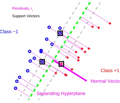
SVM performs classification by constructing a d-dimensional hyperplane that seeks to optimally separate the data into 2 categories based on certain criteria. For the separable cases, as shown in Figure 1.1, there are infinite number of lines that we can draw to separate the two classes. The SVM hyperplane (green dashed line) is oriented in such a way that the minimum distance between the separating hyperplane and the data points from each class is maximized. The minimum distance is equivalent to the distance from the green dashed line to each of the two black thin dashed lines parallel to it. This distance is also called the geometric margin. The three data points covered by black boxes on the two thin dashed lines are called the support vectors.
If we choose w∈Rd as the normal vector for our hyperplane and β ∈R to determine
its position, in general cases (not necessarily separable), the SVM analysis involves the following minimization
min
w,β,ξi
h1
2kwk
2+CX
i
ξi
i
(1.7)
Class +1
Class −1
Normal Vector
Separating Hyperplane
Residuals, r
i
Support Vectors
Figure 1.1: Illustration of SVM using a toy example. The red plus signs represent the positive class and the blue circle signs represent the negative class. The black boxes highlight the support vectors. The black dashed lines show where the functional margin is 1.
subject to:
yi(xTi w+β)≥1−ξi, ξi ≥0, for i= 1,2,· · ·, n. (1.8)
Thef unctional marginis defined to bef(x) =xTw+β. In (1.7),Cis a tuning parameter,
and the ξi, i = 1,· · · , n are slack variables for handling nonseparable data. Intuitively,
the sign of f(x) is used to classify a new unseen example x. The larger the C, the higher the penalty for violation of separability. Thus, C should be chosen with care to avoid overfitting.
One important feature of SVM is that only the support vectors, i.e. the points falling exactly on the hyperplanes which satisfy f(x) = 1 and the violated points with ξi > 0,
Distance Weighted Discrimination
Recently, Marron et al. (2007) proposed a new binary classification method, Distance Weighted Discrimination (DWD) which is specifically designed for High Dimension Low Sample Size (HDLSS) situations. DWD has similar performance to SVM when the number of samples is larger than the number of dimensions, but performs better than SVM in HDLSS cases. Like SVM, DWD is also a large margin classifier method and performs classification tasks by constructing a hyperplane in a multidimensional space that separates the two classes. The DWD hyperplane is constructed by minimizing the sum of the inverses of perpendicular distances from a candidate for the hyperplane to the data points. Suppose the separating hyperplane is expressed asxTw+β = 0, then (w, β) can be found by solving
the optimization problem,
min
w,β,ξ
n
X
i=1
³1
ri
+Cξi
´
, (1.9)
subject to:
ri =yi(xTi w+β) +ξi for i= 1,· · ·, n, kwk2 ≤1, (1.10)
ri ≥0, ξi ≥0 for i= 1,· · · , n. (1.11)
DWD is different from SVM in that it seeks to maximize a notion of average distance instead of only the minimum distance between the two classes. Thus, DWD allows all data points (ξi ≥ 0) rather than just those support vectors to have a direct impact on
the separating hyperplane. It gives high significance to those points that are close to the hyperplane, with little impact from points that are farther away. The computation of the DWD is based on Second Order Cone Programming (SOCP), a modern computationally intensive optimization method (see http://www.math.nus.edu.sg/ mattohkc/sdpt3.html for an update software for doing this).
1.3
Kernel Space
Among the set of all classification methods, the linear methods are an important and widely studied family. The linear classification rule can be obtained as ˆG(x) = signf(x) based on the function f(x) which is a linear combination of the input features x. The linear classification methods are convenient because they have simple functional forms and the relative contribution of each covariate is easy to interpret.
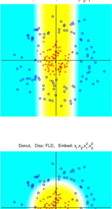
However, in practice, the true decision boundary will frequently be quite nonlinear in x as shown in Figure 1.2. The appealing kernel approach to going beyond linearity is to enlarge the feature space with additional variables, which are transformations of x, and then use linear methods in this new space. This idea is illustrated by Figure 1.2 where FDA is applied to a simple two-dimensional toy example. Note that the results based onx1, x2
only (upper-left panel) are not able to effectively capture the class difference in this case. The performances will be improved as more variables are added to the model as shown in the other three panels in Figure 1.2. Adding x21 (upper-right panel) or x22 (lower-left
panel) alone offers significant improvement over linear method while adding bothx2
1andx22
leads a much more improved decision boundary which almost makes a perfect separation between the two classes.
Lethm(x) :Rd→Rdenote themth transformation also called thebasis transf ormation
of x, m = 1,· · · , M. Once the basis functions hm have been determined, linear
classifi-cation can be performed on the hm. We fit the classifier using input features h(x) =
(h1(x),· · · , hM(x)), and produce the (nonlinear) function ˆf(x) =h(x)Tβˆ + ˆβ0. The
clas-sifier is ˆG(x) = sign( ˆf(x)) as before. Generally linear boundaries in the enlarged space achieve better training-class separation, and translate to nonlinear boundaries in the orig-inal space.
Figure 1.2: Illustration of the kernel embedding idea using a two-dimensional toy exam-ple. The four panels use different polynomial embedding. The white band represents the decision boundary. The two classes are represented by red plus and blue circle symbols. Re-sults shown in the four panels are obtained by using variablesx1, x2 (upper-left), x1, x2, x21
(upper-right), x1, x2, x22 (lower-left), and x1, x2, x21, x22 (lower-right), respectively.
a challenge. Also with sufficient basis functions, the data will nearly always be separable, and there will be large potential for overfitting. Many classification methods attempt to address this overfitting problem using some form of regularization.
We first use SVM as an example to show how to implement this basis transformation using the kernel trick and then cast it into the larger context of regularization methods to deal with overfitting. The SVM optimization problem (1.7) can be presented in such a way that the input feature space only appears in terms of inner products. We describe this using the transformed feature vectors h(x). The Lagrange dual function of (1.7) with xreplaced by h(x) has the form
LD = n
X
i=1
αi−
1 2
n
X
i=1
n
X
i′=1
αiαi′yiyi′hh(xi),h(xi′)i. (1.12)
The solution function can be written as
f(x) =
n
X
i=1
αiyihh(x),h(xi)i+β0. (1.13)
So both (1.12) and (1.13) involve h(x) only through inner products. Thus we don’t need to specify the transformation h(x), but only need to know the kernel function K(x,x′) =
hh(x), h(x′)i that computes inner products in the transformed space. HereK should be a
symmetric positive (semi-) definite function.
It is well known that many important classification methods can be fit in a general class of regularization problem of the form written as solutions to
min
f∈H
hXn
i=1
L(yi, f(xi)) +λJ(f)
¤
, (1.14)
Suppose that the f in (1.14) lives in a reproducing kernel Hilbert space (RKHS) HK
generated by a positive definite kernel K(x,x′). Further define the penalty functional for
the space HK to be the squared norm J(f) =kfk2HK. Then (1.14) can be written as
min
f∈HK
hXn
i=1
L(yi, f(xi)) +λkfk2HK ¤
. (1.15)
It can be shown using the representer theorem (Wahba (1990)) that the solution to (1.15) is finite-dimensional, and has the form f(x) = Pni=1αiK(x,xi). This approach is called
the kernel trick.
Using the kernel trick, a linear algorithm can easily be transformed into a non-linear algorithm by mapping the data into a high dimensional feature space. This non-linear algorithm is equivalent to the linear algorithm operating in that space. The nice feature of the kernel trick is that it enables us to operate in the new space without ever computing the coordinates of the data in that space, but rather by simply computing the inner products of the base functions between all pairs of data in the original feature space. This operation is often computationally cheaper than the explicit computation of the coordinates.
If the kernel function is chosen to be K(x,x′) = hx,x′i, the corresponding kernel space
is equivalent to the original feature space. Some commonly used kernel functions include:
• lth Degree polynomial: K(x,x′) = (1 +hx,x′i)l,
• Radial basis: K(x,x′) = exp(−kx−x′k2/c),
• Neutral network: K(x,x′) = tanh(κ
1hx,x′i+κ2).
The kernel space corresponding to the first choice is finite-dimensional and the kernel spaces corresponding to the second and third choices are infinite-dimensional. Algorithms capable of operating with kernel tricks include LDA, SVM, DWD and many others.
1.4
Bi-Directional Discrimination
Linear classifiers are simple and easy to interpret, but can suffer some serious limi-tations in the complicated situations. Kernel learning enables us to easily generalize the linear classifiers to nonlinear classifiers and improve the classification error rates. A poten-tial trade off is that nonlinear classifiers may not give clear interpretation of the results in terms of the original features. Motivated by these concerns, we propose the Bi-Directional Discrimination (BDD) classification method in Chapter 2 which generalizes the classifi-cation boundary from using only one hyperplane to using two hyperplanes. The BDD method is anticipated to be more effective in the cases where the classes have distinct sub-populations.
In Section 2.2, we use SVM and DWD to illustrate how to generalize one-direction methods to the proposed BDD method. It is important to note that the generalization can apply to any other linear classification methods as well. The optimization problems for the BDD method involve replacing the linear function f(x) = xTw+β (in the linear classification methods) by the product of two linear functions f1(x)f2(x), where f1(x) =
xTw
1+β1 andf2(x) =xTw2+β2. As a consequence, we have two separating hyperplanes
instead of one. The classification rule can be stated as ˆG(x) = sign( ˆf1(x) ˆf2(x)), i.e., points
in the regions ˆf1(x) > 0, ˆf2(x) > 0 or ˆf1(x) < 0, ˆf2(x) < 0 are labeled as belonging to
the positive class while points in the regions ˆf1(x)>0, ˆf2(x)<0 or ˆf1(x)<0, ˆf2(x)>0
are labeled as belonging to the negative class. The two directions introduced in the BDD method can also provide a visualization tool for HDLSS data.
It is difficult to solve the optimization problems which involve the form f1(x)f2(x) for
(w1, β1) and (w2, β2) simultaneously. In Section 2.2.2, we propose an iterative algorithm
classification problem. Then the other hyperplane can be solved from this transformed problem. This procedure is repeated until convergence is achieved.
Like many iterative algorithms, local minima are also a serious concern here especially in the HDLSS situations. Thus how to choose proper initial values will become an important issue. In Section 2.2.3, we propose four methods for choosing initial values based on two different considerations. We call the four methods Cluster1-1, Cluster2-2, Cluster1-2 and FullQuadProj respectively. The first three methods choose the initial values by considering the different subcluster situations within each class. The last method chooses the initial values by finding the two hyperplanes which best approximate an appropriate full quadratic kernel method. For each method, there are situations in which it performs better than the others.
The proposed BDD method is studied in Section 2.3 through several simulations and two real data examples. The performances of various initial value methods are evaluated using data visualization and careful studies of the test errors (for simulated data) and cross-validation errors (for real data). Comparison with the usual one-direction linear classification methods is also included. The numerical results show that in contrast to the one-direction methods, the BDD method is competitive for different data settings and gives major improvement in the case when there are distinct subclusters within each class.
In Section 2.3.2, we study the asymptotic properties of the BDD method in the limit as d → ∞ with the sample size n fixed. This is different from the classic asymptotics which is in the limit as n → ∞. We give the asymptotic geometric representations of the data set which include subclusters. We also study when the BDD method performs better than the usual one-direction classification methods.
1.5
Multiclass Classification
Summary of Existing Multiclass Classification Methods
Now turn our attention to the multicategory classification problem. Binary classifica-tion is a well studied special case. In practice, multicategory problems are important as well. Binary classification methods can be generalized in many ways to handle multiple classes. Some multicategory classification methods are straightforward extension of binary ideas such as kNN, neural network, LDA, and logistic regression discussed in Section 1.2. However, the extension from binary to multicategory case is more challenging for others.
The generalization of the kNN method is straightforward. In the multicategory case, one first finds thekclosest objects from the training sample to a new object being classified, then assign this object to the class which appears most frequently among thesekneighbors. For the neural network method, the generalization needs to introduce K functions fk, for
k = 1,· · · , K, which are defined as
Tk = β0k+βTkZ, k= 1,· · · , K,
fk(X) = gk(T), k = 1,· · · , K.
The unknown parameters can be solved in the same way as for the binary case. The corresponding classifier is ˆG(x) = argmaxkfˆk(x). The extension of the LDA classifier can
be implemented using the following steps. First compute the pooled within class covariance
Σw = K
X
k=1
and use it to transform the data
˜
Xk = Σ−w1/2Xk, for k = 1,· · · , K. (1.17)
Then label a new object according to the closest class centroid of the training data in the transformed space. The generalization of logistic regression can be carried out by modeling the posterior probabilities of K classes as
P(G=k|X =x) = exp(βk0+β
T kx)
1 +PKl=1−1exp(βl0 +βTl x)
, k= 1,· · ·, K −1, (1.18)
P(G=K|X =x) = 1
1 +PKl=1−1exp(βl0 +βTl x)
. (1.19)
The classifier is ˆG(x) = argmaxkpk(x; ˆθ) with pk(x;θ) = P(G=k|X =x).
Multiclass SVM and DWD
The generalization from the binary case to the multicategory case for large margin clas-sification methods like SVM and DWD requires careful consideration. There are a number of different multicategory extensions of SVM in the literature. However, the extension of the DWD method has not been studied previously. We have developed several DWD extension methods in Chapter 3 and studied some statistical issues associated with them.
Two general strategies are commonly used to tackle multicategory SVM problem. One strategy is to solve the multicategory problem by solving a series of binary problems. The second one treats the population in a simultaneous fashion and considers all classes at once in a single optimization problem. Various aggregation of all pairwise classifiers and one-versus-the-rest approaches are the first strategy (Duda et al. (2000); Hastie et al. (2009)). Various extension methods along the line of the second strategy include Lee et al. (2004); Weston and Watkins (1999); Crammer and Singer (2000); Liu and Shen (2006). Following
the SVM results, our work involves the study of the extension of DWD from the binary case to the multicategory case using both strategies. We make comparisons among various methods and settings by extensive simulated data and real data applications.
CHAPTER 2
Bi-Directional Discrimination with
Application to Data Visualization
2.1
Introduction
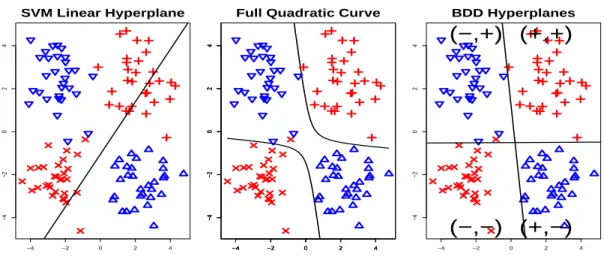
As noted in Section 1.4, while linear classifiers have been very widely used, there is an important collection of problems where they can be dramatically improved upon. This is illustrated in Figure 2.1. In this case, each class contains diverse sub-populations. For example, in microarray analysis, within each class of interest (e.g., disease versus control) immaterial differences such as male versus female can lead to diverse sub-populations. A toy example illustrating this is given in Figure 2.1 which shows a scatter plot of two dimensional data. The positive and negative classes are represented as red and blue respectively. Each class is further divided into two sub-clusters which are distinguished using different symbols in the scatter plot. The linear SVM model is fit to these data and its decision boundary is denoted by the solid line in the left panel of Figure 2.1. Note that linear methods for classification are not able to effectively capture the class difference in this case which motivates us to find a more general hypersurface that can divide the two classes of samples.
−4 −2 0 2 4
−4
−2
0
2
4
SVM Linear Hyperplane
−4 −2 0 2 4
−4
−2
0
2
4
Full Quadratic Curve
−4 −2 0 2 4
−4
−2
0
2
4
−4 −2 0 2 4
−4
−2
0
2
4
−4 −2 0 2 4
−4
−2
0
2
4
BDD Hyperplanes
(+,+)
(+,−)
(−,−)
(−,+)
Figure 2.1: Toy data example in two dimensions with three different discrimination curves shown using a solid line-type. Red color (plus and “x” symbols’) indicates the positive class and blue color (up and down triangles) indicates the negative class. Different symbols in the same class represent different sub-clusters. Note the two non-linear methods give (middle and right panels) major improvements.
linear case to the non-linear case is allowed and quite straightforward using the kernel trick (Aizerman et al. (1964); Boser et al. (1992)). This is accomplished by mapping the data to a high-dimensional space where the classification is achieved via a linear classifier, and then by mapping the results back to the original feature space. This results in a non-planar hypersurface that can be more adapted to the complexity of the interface between the two classes, and thus is more effective. The solid curves in the middle panel of Figure 2.1 are the non-linear decision boundary implemented using the full quadratic kernel method (Vapnik (1995); Burges (1998)). Its performance is clearly much better than that of the linear classifier.
higher than that of the original feature space and thus tend to be far more prone to serious overfitting in high dimensions. In order to get around these problems and be able to display class differences in a way that is not only effective, but also suitable for visual interpretation of the data, we develop a new classification method in this dissertation, called Bi-Directional Discrimination (BDD). The basic idea of BDD is to find two (or more) linear hyperplanes instead of one to separate the two classes. The BDD decision boundary is shown in the right panel of Figure 2.1 which does a more intuitively appealing job of separating the two classes since it not only provides good between-class separation but also clearly divides each class into two sub-clusters.
The BDD method has big advantages over general non-linear methods especially for HDLSS data. HDLSS data are becoming increasingly common in various fields including genetic microarrays, medical imaging and chemometrics, etc. If the dimension is d, the number of parameters included in the BDD method will be 2d, much less than that included
in the quadratic kernel method which is at least
d
2
. As a consequence of its simplicity,
the overfitting problem for the full quadratic kernel illustrated in Section 2.3 is greatly reduced by BDD. Another important feature of our BDD method is that its two hyperplanes can automatically provide a visualization tool for HDLSS data. For many tasks of HDLSS data analysis, visualization plays an important role. This is key for efficient integration of human expertise - not only to include background knowledge, intuition and creativity, but also the powerful human pattern recognition and processing capability (Walter (2004)). Therefore, studying the projections of the data points onto the two directions solved by our BDD approaches can help us obtain more insights from the data, and thus reveals a whole new family of methods between the simple one-direction linear methods and the full general non-linear methods.
Other approaches in the literature also have the potential to address the subcluster
problem that is tackled by BDD. For example, Gaussian mixture models (see e.g. Hastie and Tibshirani (1996)) have the flexibility to associate Gaussian mixture components to each subclass to facilitate effective classification when the classes have subpopulation. But they are not suitable for high dimensional analysis, which is the main motivation of BDD. Classification and Regression Trees (CART) and more advanced tree methods (Breiman et al. (1984)) can tackle very high dimensions, but are much less flexible than BDD because they only allow splits in coordinate directions.
In this chapter, we initially focus on the two-directional method. We also generalize BDD to multiple directions. In particular, we discuss the three-directional method as well as its implementation. Moreover, although our BDD method is motivated by the SVM and DWD methods, we note that the fundamental concept is more general and can be applied to the extension of any other linear classifier as well. In this dissertation, we only focus on the discussion of the SVM and DWD methods and use them as examples to illustrate how the BDD method works.
2.2
Bi-Directional Discrimination Framework
This section gives the details of how to generalize the 1SVM and 1DWD methods from the usual one-direction case to the two-direction case. Let us first set the notation to be used. Suppose that the training data set consists of n d-vectors xi together with
corresponding class indicators yi ∈ {+1,−1}, which are distributed according to some
unknown probability distribution functionP(x,y).
2.2.1
Review of Uni-Directional Methods
The main idea behind the classical one-direction classification problem in the separable case is to find the separating hyperplane with maximum separation between the two classes. More specifically, the 1SVM hyperplane maximizes the distance between the hyperplane and the closest data point of each class, while the 1DWD hyperplane minimizes the sum of the reciprocals of the distances from every data point to the separating hyperplane. One important goal is to do prediction, i.e., if we choose w∈ Rd as the normal vector for our
hyperplane and β ∈ R to determine its position, the sign of f = xTw+β can be used
for prediction of class labels for new inputs x. The optimization problems, for both the 1SVM and 1DWD approaches, depend on the signed distance from each data point to the decision boundary, which is defined as
ri0 = yi(xTi w+β), i= 1· · · , n. (2.1)
If separation between the two classes is not feasible, we need to add perturbation terms to make sure that all residuals are positive (Cortes and Vapnik (1995)). We obtain
ri = yi(xTi w+β) +ξi, (2.2)
where the slack variable ξi ≥ 0, and the equality holds when the data vector xi lies on
the correct side of the separating hyperplane. The hyperplane parameters (w, β) can be determined to encourage all ri to be positive and large. The 1SVM classifier solves the
regularization problem
min{w,β}
Ã
1 2||w||
2+C
1SV M n
X
i=1
ξi
!
, (2.3)
subject to yi(xTi w+β) +ξi ≥ 1 and ξi ≥ 0, where C1SV M > 0 is the penalty parameter,
which balances the separation and the amount of violation of the constraints. Here ||w|| refers to the Euclidean norm of w.
The optimization formula (2.3) is the primal problem of the 1SVM. Using Lagrange multipliers, it can be converted to an equivalent dual problem as follows
minα
Ã
1 2
n
X
i,j=1
yiyjαiαjhxi,xji − n
X
i=1
αi
!
, (2.4)
subject to Pni=1yiαi = 0; 0 ≤ αi ≤ C1SV M, ∀i. This convex optimization problem has
quadratic objective function and linear constraints and can be easily solved. Once the solution of (2.4) is obtained, w can be calculated as Pni=1yiαixi, and β can be computed
using the Karash-Kuhn-Tucker (KKT) conditions of the optimization theory (Fletcher (1987)).
The optimization task of 1DWD is to find a separating hyperplane which solves
min{w,β}
X
i
µ
1 ri
+C1DW Dξi
, (2.5)
subject to ri = yi(xTi w+β) +ξi ≥ 0, ||w||2 = 1 and ξi ≥ 0, where C1DW D > 0 is the
and is subject to linear constraints with the requirement that various sub-vectors of the decision vector must lie in second-order cones. SOCP problems have also been extensively studied and there exist well established algorithms for solving them, see Alizadeh et al. (2001). The dual problem of 1DWD can also be described in terms of the SOCP settings. Both primal and dual problems of 1DWD have optimal solutions. For detailed description of 1DWD formulation and optimization, we refer to the original 1DWD paper (Marron et al. (2007)).
2.2.2
Bi-Directional Discrimination
In the two-direction case, we have two hyperplanes represented by parameters (w1, β1)
and (w2, β2) respectively. Letf1 =xTw1+β1andf2 =xTw2+β2be classification functions
representing each of the two separating hyperplanes (as f1 = 0 and f2 = 0). As shown in
the right panel of Figure 2.1, we denote by (+,+) the region which satisfies f1 > 0 and
f2 > 0. The other three regions can be denoted in a similar way. It turns out that the
data from the positive class tend to be located on the upper-right and lower-left regions with labels (+,+) and (−,−) while the data from the negative class tend to lie in the upper-left and lower-right regions with labels (−,+) and (+,−). Thus sign(f1f2) is used
as the predicted rule in the two-direction setting. Therefore, a natural way of generalizing linear classifiers is to replace the signed distance ri of the ith data point (2.2) with
si = yif1f2+ξi. (2.6)
Once the si are given, the optimization problem solved by the two-direction SVM can be
stated as
minw,β,ξ
1 2(||w1||
2+
||w2||2) +CSV M n
X
i=1
ξi (2.7)
subject to
si =yi(xTi w1 +β1)(xTi w2+β2) +ξi ≥1, ξi ≥0. (2.8)
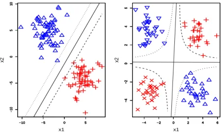
The illustration plots for one-direction SVM and two-direction SVM are shown in the left panel and the right panel of Figure 2.2 respectively. The decision boundary of two-direction SVM consists of two lines. The curves defined by yf1f2 = 1 are four hyperbolas
which correspond to the two lines defined by yf = 1 in the one-direction plot. Thus two-direction SVM seeks to choose two hyperplanes to maximize the distances between the four hyperbolas that are as far apart as possible. The data points which lie on the four hyperbolas are the support vectors for two-direction SVM.
−10 −5 0 5
−10 −5 0 5 10 x1 x2
−10 −5 0 5
−10
−5
0
5
10
−10 −5 0 5
−10
−5
0
5
10
−10 −5 0 5
−10
−5
0
5
10
−4 −2 0 2 4 6
−4 −2 0 2 4 6 x1 x2
−4 −2 0 2 4 6
−4 −2 0 2 4 6
−4 −2 0 2 4 6
−4 −2 0 2 4 6
−4 −2 0 2 4 6
−4 −2 0 2 4 6
−4 −2 0 2 4 6
−4 −2 0 2 4 6
Figure 2.2: Illustration plots for both one-direction SVM (left panel) and two-direction SVM (right panel). Solid lines represent decision boundaries. Dashed and dotted lines in the left panel are defined by f = 1 and f = −1 respectively. Dashed curves and Dotted curves in the right panel are defined by f1f2 = 1 and f1f2 =−1 respectively.
Similarly, the optimization problem solved by the two-direction DWD can be stated as
minw,β,ξ
X
i
µ
1 si
+CDW Dξi
subject to
si =yi(xTi w1+β1)(xiTw2+β2) +ξi ≥0, ξi ≥0,
||w1||2+β21 = 1,||w2||2 +β22 = 1. (2.10)
To meet the uniqueness requirement, here we use the constraints ||wj||2 +βj2 = 1 instead
of ||wj||2 = 1, j = 1,2, as used in the original 1DWD method. We choose this type of
constraint to ensure that the optimization problem can be described in SOCP terms.
The multiplicative form of the si in (2.6) poses significantly greater optimization
chal-lenges and makes it difficult to simultaneously solve for (w1, β1) and (w2, β2) both in (2.7)
and in (2.9). However, we note that as long as one of the two hyperplanes is given, (2.7) and (2.9) can be solved for the other hyperplane using methods similar to the ordinary 1SVM and 1DWD. This property suggests that iterative algorithms can be used here. Therefore we propose to solve the two-direction minimization problem by minimizing a sequence of one-direction sub-problems. We can proceed as follows. First propose initial values for {w1(0), β1(0)}. Then obtain {w(0)2 , β2(0)} by solving the revised 1SVM and 1DWD problems with yi replaced by ˆyi = yi(xTi w
(0)
1 +β
(0)
1 ). Then based on {w (0) 2 , β
(0)
2 } we can
obtain {w(1)1 , β1(1)} and repeat this process until convergence of both parameters. Thus, a solution can be achieved by alternately updating each hyperplane based on each fixed value of the other one. In each iteration, we only need to solve the modified 1SVM or 1DWD problems whose response values are continuous (ˆyi) instead of binary (yi). In all
cases we considered, this algorithm converges in at most 10 steps.
2.2.3
Starting Points
Local minima can be a serious concern for iterative optimization methods. The solution based on the iterative algorithm described in Section 2.2.2 strongly depends on the choice of
the initial values {w1(0), β1(0)}. Different initial values may end up with different solutions. Especially for high dimensional situations, the objective functions can have many local minima due to the complexity of their special multiplicative form. Figure 2.3 shows the distribution of the final (after convergence of the iterative algorithm) objective function values based on a single realization of a simulated data set with d=1000. Details of this simulation are discussed in Section 2.3.2. The blue kernel density estimation (KDE) plot is derived from 1000 samples of objective function values, each of which is calculated based on one randomly selected starting point. The vertical lines with different colors represent the results derived from some special initial points. Here MIN-RAND represents the minimum values among the 1000 random simulations and the other notations will be discussed in detail in this section. Figure 2.3 illustrates how crucial the starting points are to our optimization algorithm. Our next goal is to propose some appropriate ways to choose good initial values.
These ideas are effectively illustrated using a set of 3 two-dimensional toy examples de-scribed in Section 2.2.3.1. An approach to starting values based on the full quadratic kernel embedding is developed in Section 2.2.3.2. An alternative approach, based on clustering, is given in Section 2.2.3.3.
2.2.3.1 Toy Examples
Since one of the motivations of our two-direction classification method comes from the fact that there might be further sub-clusters within each class, we can illustrate our methods using examples as shown in Figure 2.4 where three types of 2-dimensional data sets are generated from normal distributions with different means.
Example 1 (4-Cluster-Twisted):
2 3 4 5 6 7 8 9 10 11 0 0.1 0.2 0.3 0.4 0.5 FullQuadProj Cluster1−2 Cluster2−2 DWD1−START MIN−RAND
Figure 2.3: KDE plot of objective function values for different starting points.
−5 0 5
−6 −4 −2 0 2 4 6
Example 1: 4−Cluster−Twisted
+1
+2 −1 −2
−5 0 5
−6 −4 −2 0 2 4 6 +1 −2 +2 −1
Example 2: 4−Cluster−Straight
−5 0 5
−6 −4 −2 0 2 4 6
Example 3: 3−Cluster−Triangle
+1 −1
+2
Figure 2.4: Illustration of some different sub-cluster situations for binary classification problems. Red color (plus and “x” symbols’) indicates the positive class and blue color (up and down triangles) indicates the negative class. Different symbols in the same class represent different sub-clusters.
for each class. The four clusters are sampled from four shifted standard bi-variate normal distributions whose means are (µ, µ), (−µ, µ), (−µ,−µ), and (−µ, µ) with µ = √5. We label the four distinct clusters as +1 (red plus sign), +2 (red “x” sign), −1 (blue down-triangle), −2 (blue up-triangle) as shown in the plot. Clusters +1 and +2 (centered in the upper right and lower left quadrants) belong to the positive class and clusters −1 and −2 (centered in the upper left and lower right quadrants) belong to the negative class. The
numbers of individuals in each cluster are 25.
Example 2 (4-Cluster-Straight):
This example is shown in the plot (b) of Figure 2.4 which also includes four clusters whose means are (µ, µ), (−µ, µ), (−µ,−µ), and (−µ, µ) with µ=√5 and identity covari-ance. In this example, clusters +1 and +2 (centered in the upper right and lower right quadrants) belong to the positive class and clusters−1 and−2 (centered in the upper left and lower left quadrants) belong to the negative class. The numbers of individuals in each cluster are 25.
Example 3 (3-Cluster-Triangle):
This example is shown in the plot (c) of Figure 2.4 where only the positive class includes two sub-clusters. Thus we have three shifted standard Gaussian clusters whose means are (µ,0), (−µ,0), and (0, µ) with µ = √5. We label the three distinct clusters as +1 (red plus sign), +2 (red “x” sign) and−1 (blue up-triangle). Clusters +1 and +2 belong to the positive class and cluster −1 belongs to the negative class. Here n+1 =n+2 =n−1/2 = 25,
which means that the total number of individuals in the positive class is equal to that in the negative class.
2.2.3.2 Full Quadratic Kernel Approach
extension from the linear case to the non-linear case can be obtained by simply replacing the vector xi by Φ(xi), where the non-linear mapping Φ is obtained from the symmetric
kernel function K by performing Cholesky factorizationK(xi,xj) = Φ(xi)TΦ(xj). This is
equivalent to solving the linear problem in the feature space induced by the kernel K to achieve the nonlinear solution in the original space. We choose the second order polynomial kernel function which is of the form
K(xi,xj) = (1 +hxi,xji)2. (2.11)
Once we get the non-linear classification function evaluated at each data point
¯
yi = Φ(xi)Tw¯ + ¯β, (2.12)
we can find the approximate solutions of (2.7) and (2.9) by minimizing the following residual sum-of-squares
n
X
i
(¯yi−(xTi w1 +β1)(xTiw2+β2))2. (2.13)
Using these solutions as initial values, we can proceed with the iterative method to get the final solution. It is also difficult to find a simple closed form solution to the optimization problem (2.13). However, since it has nice properties in the sense that both function values and derivatives can be analytically evaluated, the solution can be obtained using standard numerical optimization algorithms. We use conjugate gradient methods from Fletcher (1987) to solve this.
2.2.3.3 Clustering Approach
Our second type of initialization approach is proposed on the basis of the sub-cluster structure of the data set. We use the three examples given in Section 2.2.3.1 as a simple illustration for this.
For Example 1 (4-Cluster-Twisted), the ideal choice for the initial hyperplane will be the one-direction hyperplane that separates groups (+1,−1) and (+2,−2) or else the one that separates groups (+1,−2) and (+2,−1). Therefore, our Cluster2-2 method first uses 2-means clustering algorithm to divide the positive class into two clusters labeled as c+1
and c+2 and similarly divides the negative class into two clusters labeled as c−1 and c−2.
Then we choose the initial hyperplane as the usual one-direction hyperplane that either separates between groups (c+1, c−1) and (c+2, c−2) or separates between groups (c+1, c−2)
and (c+2, c−1).
For Example 2 (4-Cluster-Straight), it is better to choose the usual one-direction linear classifier as an initial value. Thus, our Cluster1-1 method chooses the usual one-direction hyperplane between the positive and the negative classes as the initial value.
For Example 3 (3-Cluster-Triangle), a good choice of the initial value is the one-direction hyperplane that separates groups (+1) and (+2,−1) or the one that separates groups (+2) and (+1,−1). Our Cluster1-2 method using the 2-means clustering algorithm divides the positive class into two clusters labeled as c+1, c+2. The initial hyperplane is chosen to be
the one that separates either between groups (c+1) and (c+2, c−1) or between groups (c+2)
and (c+1, c−1), where c−1 denotes the entire negative class.
2.2.4
More Than Two Directions
Although our focus is this dissertation is on the two-directional method, it can be extended to multiple directions. To generalize BDD to theK-direction case, discrimination is based onK hyperplanes represented by parameters (w1, β1),· · ·, (wK, βK) respectively.
Letfi =xTwi+βi, fori= 1,· · · , K be classification functions representing each of the K
separating hyperplanes (i.e. fi = 0, i = 1,· · · , K). The class label for a new input x is
predicted to be sign(f1(x)· · ·fK(x)). The optimization problem in (2.7) and (2.8) can be
written as
minw,β,ξ
1 2
K
X
j=1
||wj||2+CSV M n
X
i=1
ξi (2.14)
subject to
si =yi K
Y
j=1
(xTjwj +βj) +ξi ≥1, ξi ≥0.
The DWD problem can be described in a similar way.
The optimization problem (2.14) can be solved using an iterative algorithm similar to the BDD case. Now the choice of initial values is more challenging because we need to chooseK−1 initial directions. We only briefly explain the case withK = 3 here. For the Tri-Direction Discrimination (TDD) problem, we need to choose two initial hyperplanes. For each class (“+” or “−”) we consider three cases in terms of subclusters:
• All data lie in a single, well defined cluster (labeled as (+) or (−)).
• The data in the class lie in exactly two distinct subclusters (labeled as (+I,+II) or (−I,−II)).
• The data in the class lie in three or more clusters (labeled as (+1,+2,+3) or (−1,−2,−3)), where clusters are appropriately combined when there are more than 3).
We recommend choosing the initial two hyperplanes based on the consideration of the following clustering:
1. Cluster1-1: BDD output for (+) versus (−) using the Cluster1-2 method.
2. Cluster1-2: BDD output for (+I,+II) versus (−) or for (+) versus (−I,−II) using Cluster1-1 method.
3. Cluster1-3: get BDD output for all pairwise classification problems of the form (±) versus (∓i,∓j) for i, j = 1,2,3 using the Cluster1-2 method and choose the one which gives the lowest TDD objective function value.
4. Cluster2-2a: BDD output for (+I,+II) versus (−I,−II) using the Cluster2-2 method. 5. Cluster2-2b: get the BDD output for all pairwise classification problems of the form
(±I) versus (∓I,∓II) using the Cluster1-2 method and choose the one which gives the lowest TDD objective function value.
6. Cluster2-3: get the BDD output for all such classification problems as (±I,±II) versus (∓i,∓j) for i, j = 1,2,3 using the Cluster2-2 method and choose the one which gives the lowest TDD objective function value.
7. Cluster3-3: get the BDD output for all pairwise classification problems of the form (±i,±j) versus (∓i′,∓j′) for i, j, i′, j′ = 1,2,3 using the Cluster2-2 method and
choose the one which gives the lowest TDD objective function value.
As in Section 2.2.3, the finally selected method of TDD is that which minimizes the objec-tive value. In Section 2.3.3, we will demonstrate TDD using two simulated examples.
2.3
Visualization, Simulation and Data Analysis
sets in Section 2.3.1 and then to simulated high dimensional data sets in Section 2.3.2. We apply our TDD method to simulated data sets in Section 2.3.3. The application of the BDD method to two real data sets is discussed in Section 2.3.4. In Sections 2.3.1, 2.3.2 and 2.3.3, we set the sample sizes of training and test data as 100 and 1000, respectively. We generated the test data from the same distributions as the training data. Both the DWD and SVM methods were used in the numerical calculations and their results were quite similar. Due to space limitations, only DWD results are reported here.
A simple recommendation for the choice of the 1DWD tuning parameter was made in Marron et al. (2007) as C1DW D = 100/d2t, where dt is the median of the pairwise between
class Euclidean distances. This simple default value of the tuning parameter is implemented by most users and has been shown to work well (Qiao et al. (2010)). For BDD we found this simple default approach to tuning was not as reliable as in the case of 1DWD. It was adequate in our simulated example, so we used it to reduce the computational burden in Sections 2.3.1 and 2.3.2. However, it gave an inferior result for the real data sets in Section 2.3.4, so we use cross-validation (CV) there, and recommend this in general.
2.3.1
Simulated Low Dimensional Examples
We consider three two-dimensional simulated examples. The simulation setting here is identical to that of Section 2.2.3.1 . We apply the iterative two-direction DWD algorithms described in Section 2.2.3 to each data set. The four different initial hyperplane options (Cluster1-1, Cluster2-2, Cluster1-2 and FullQuadProj) considered in Sections 2.2.3.2 and 2.2.3.3 are used. The combined BDD solution is determined from the one that gives the minimum objective function value among the four options. Let COMBO represent this combined BDD approach which is defined as
COMBO = argmin{OBJ(Cluster1-1),OBJ(Cluster2-2),
OBJ(Cluster1-2),OBJ(FullQuadProj)}.
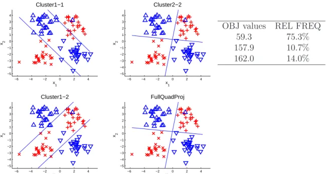
The data and the resulting two-direction hyperplanes using the four initializations are plotted in the left and middle panels of Figure 2.5 for the 4-Cluster-Twisted example. For comparison, we also randomly simulated 1000 initial values and compute the objective function values based on each of them. The calculated objective function takes only 3 values, with frequencies shown in the table in the right panel of Figure 2.5. These 3 values correspond to three local optimal solutions which correspond to the three distinct decision boundaries shown in the left and middle panels of Figure 2.5. The Cluster2-2 and FullQuadProj methods give the same solution which corresponds to the objective value 59.3. The solutions from the Cluster1-1 and Cluster1-2 methods correspond to the other objective values 157.9 and 162.0. These two solutions are both driven by combining pairs of subgroups into a single group as their corresponding objective values are similar. The third possible way of combining subgroups (chosen by Cluster2-2 and FullQuadProj) is better, as indicated by the much smaller objective value of 59.3. It is important to note that for most of the simulated realizations, the four starting options all choose the global optimal solution. This is consistent with the high frequency of globally optimal solution shown in the table in the right panel of Figure 2.5. The realization shown in Figure 2.5 was carefully culled from the whole collection to display all three types of local optima.
−6 −4 −2 0 2 4 −5 −4 −3 −2 −1 0 1 2 3 4 Cluster1−1 x1 x2
−6 −4 −2 0 2 4
−5 −4 −3 −2 −1 0 1 2 3 4 Cluster2−2 x1 x2
−6 −4 −2 0 2 4
−5 −4 −3 −2 −1 0 1 2 3 4 Cluster1−2 x 1 x2
−6 −4 −2 0 2 4
−5 −4 −3 −2 −1 0 1 2 3 4 FullQuadProj x 1 x2
OBJ values REL FREQ
59.3 75.3%
157.9 10.7%
162.0 14.0%
Figure 2.5: Application to 4-Cluster-Twisted type of two-dimensional simulated data set. This realization was carefully chosen to show both types of local optima (left panel) and the global optimum (central panel). Observed objective values and their relative frequencies based on 1000 random starts are shown in the table (right panel).
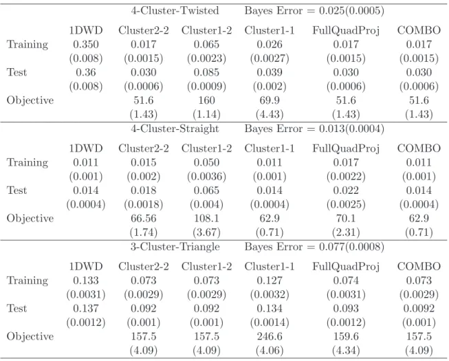
classification problem. For each example, the classification methods are assessed in terms of Training Error, Test Error (based on sets of 1000 test points as above) and the value of the objective functions. For comparison, we include in Table 2.1 the results calculated for 1DWD. Table 2.1 also includes the COMBO results using the initial values which give the minimal objective function values among the four proposed options.
Note that not all data sets are separable so that the training errors are not zero for all methods. For the 4-Cluster-Twisted example, as expected, the Cluster2-2 method per-forms the best among the three clustering based initialization methods. The FullQuadProj method gives the same performance. The Cluster1-2 method is substantially worse but it is still much better than the conventional 1DWD method. For the 4-Cluster-Straight example, the Cluster1-1 method performs the best among the three clustering based meth-ods. The performances of the Cluster2-2 and FullQuadProj methods are slightly worse. The worst one is the cluster1-2 method. The 1DWD method, as expected, works very
Table 2.1: Performance summary, average error rates over 100 simulations, of the ap-plication of the one-direction and the direction classification methods to three two-dimensional simulation examples. The numbers in the parentheses show standard errors.
4-Cluster-Twisted Bayes Error = 0.025(0.0005)
1DWD Cluster2-2 Cluster1-2 Cluster1-1 FullQuadProj COMBO
Training 0.350 0.017 0.065 0.026 0.017 0.017
(0.008) (0.0015) (0.0023) (0.0027) (0.0015) (0.0015)
Test 0.36 0.030 0.085 0.039 0.030 0.030
(0.008) (0.0006) (0.0009) (0.002) (0.0006) (0.0006)
Objective 51.6 160 69.9 51.6 51.6
(1.43) (1.14) (4.43) (1.43) (1.43)
4-Cluster-Straight Bayes Error = 0.013(0.0004)
1DWD Cluster2-2 Cluster1-2 Cluster1-1 FullQuadProj COMBO
Training 0.011 0.015 0.050 0.011 0.017 0.011
(0.001) (0.002) (0.0036) (0.001) (0.0022) (0.001)
Test 0.014 0.018 0.065 0.014 0.022 0.014
(0.0004) (0.0018) (0.004) (0.0004) (0.0025) (0.0004)
Objective 66.56 108.1 62.9 70.1 62.9
(1.74) (3.67) (0.71) (2.31) (0.71)
3-Cluster-Triangle Bayes Error = 0.077(0.0008)
1DWD Cluster2-2 Cluster1-2 Cluster1-1 FullQuadProj COMBO
Training 0.133 0.073 0.073 0.127 0.074 0.073
(0.0031) (0.0029) (0.0029) (0.0032) (0.0031) (0.0029)
Test 0.137 0.092 0.092 0.134 0.093 0.0092
(0.0012) (0.001) (0.001) (0.0014) (0.0012) (0.001)
Objective 157.5 157.5 246.6 159.6 157.5