THE High Efficiency Video Coding (HEVC) standard is

Overview of the High Efficiency Video Coding

(HEVC) Standard

Gary J. Sullivan,

Jens-Rainer Ohm,

Woo-Jin Han,

and

Thomas Wiegand,

Abstract—High Efficiency Video Coding (HEVC) is currently being prepared as the newest video coding standard of the ITU-T Video Coding Experts Group and the ISO/IEC Moving Picture Experts Group. The main goal of the HEVC standard-ization effort is to enable significantly improved compression performance relative to existing standards—in the range of 50% bit-rate reduction for equal perceptual video quality. This paper provides an overview of the technical features and characteristics of the HEVC standard.

Index Terms—Advanced video coding (AVC), H.264, High Efficiency Video Coding (HEVC), Joint Collaborative Team on Video Coding (JCT-VC), Moving Picture Experts Group (MPEG), MPEG-4, standards, Video Coding Experts Group (VCEG), video compression.

I. Introduction

T

the most recent joint video project of the ITU-T Video Coding Experts Group (VCEG) and the ISO/IEC Moving Picture Experts Group (MPEG) standardization organizations, working together in a partnership known as the Joint Col-laborative Team on Video Coding (JCT-VC) [1]. The first edition of the HEVC standard is expected to be finalized in January 2013, resulting in an aligned text that will be published by both ITU-T and ISO/IEC. Additional work is planned to extend the standard to support several additional application scenarios, including extended-range uses with enhanced pre-cision and color format support, scalable video coding, and 3-D/stereo/multiview video coding. In ISO/IEC, the HEVC standard will become MPEG-H Part 2 (ISO/IEC 23008-2) and in ITU-T it is likely to become ITU-T Recommendation H.265.

Manuscript received May 25, 2012; revised August 22, 2012; accepted August 24, 2012. Date of publication October 2, 2012; date of current version January 8, 2013. This paper was recommended by Associate Editor H. Gharavi. (Corresponding author: W.-J. Han.)

G. J. Sullivan is with Microsoft Corporation, Redmond, WA 98052 USA (e-mail: [email protected]).

J.-R. Ohm is with the Institute of Communication Engineering, RWTH Aachen University, Aachen 52056, Germany (e-mail: [email protected]).

W.-J. Han is with the Department of Software Design and Management, Gachon University, Seongnam 461-701, Korea (e-mail: [email protected]). T. Wiegand is with the Fraunhofer Institute for Telecommunications, Hein-rich Hertz Institute, Berlin 10587, Germany, and also with the Berlin Institute of Technology, Berlin 10587, Germany (e-mail: [email protected]).

Color versions of one or more of the figures in this paper are available online at http://ieeexplore.ieee.org.

Digital Object Identifier 10.1109/TCSVT.2012.2221191

Video coding standards have evolved primarily through the development of the well-known ITU-T and ISO/IEC standards. The ITU-T produced H.261 [2] and H.263 [3], ISO/IEC produced MPEG-1 [4] and MPEG-4 Visual [5], and the two organizations jointly produced the H.262/MPEG-2 Video [6] and H.264/MPEG-4 Advanced Video Coding (AVC) [7] stan-dards. The two standards that were jointly produced have had a particularly strong impact and have found their way into a wide variety of products that are increasingly prevalent in our daily lives. Throughout this evolution, continued efforts have been made to maximize compression capability and improve other characteristics such as data loss robustness, while considering the computational resources that were practical for use in prod-ucts at the time of anticipated deployment of each standard.

The major video coding standard directly preceding the HEVC project was H.264/MPEG-4 AVC, which was initially developed in the period between 1999 and 2003, and then was extended in several important ways from 2003–2009. H.264/MPEG-4 AVC has been an enabling technology for dig-ital video in almost every area that was not previously covered by H.262/MPEG-2 Video and has substantially displaced the older standard within its existing application domains. It is widely used for many applications, including broadcast of high definition (HD) TV signals over satellite, cable, and terrestrial transmission systems, video content acquisition and editing systems, camcorders, security applications, Internet and mo-bile network video, Blu-ray Discs, and real-time conversa-tional applications such as video chat, video conferencing, and telepresence systems.

However, an increasing diversity of services, the grow-ing popularity of HD video, and the emergence of beyond-HD formats (e.g., 4k×2k or 8k×4k resolution) are creating even stronger needs for coding efficiency superior to H.264/ MPEG-4 AVC’s capabilities. The need is even stronger when higher resolution is accompanied by stereo or multiview capture and display. Moreover, the traffic caused by video applications targeting mobile devices and tablet PCs, as well as the transmission needs for video-on-demand services, are imposing severe challenges on today’s networks. An increased desire for higher quality and resolutions is also arising in mobile applications.

HEVC has been designed to address essentially all existing applications of H.264/MPEG-4 AVC and to particularly focus on two key issues: increased video resolution and increased use of parallel processing architectures. The syntax of HEVC 1051-8215/$31.00 c2012 IEEE

is generic and should also be generally suited for other applications that are not specifically mentioned above.

As has been the case for all past ITU-T and ISO/IEC video coding standards, in HEVC only the bitstream structure and syntax is standardized, as well as constraints on the bitstream and its mapping for the generation of decoded pictures. The mapping is given by defining the semantic meaning of syntax elements and a decoding process such that every decoder conforming to the standard will produce the same output when given a bitstream that conforms to the constraints of the standard. This limitation of the scope of the standard permits maximal freedom to optimize implementations in a manner appropriate to specific applications (balancing compression quality, implementation cost, time to market, and other con-siderations). However, it provides no guarantees of end-to-end reproduction quality, as it allows even crude encoding techniques to be considered conforming.

To assist the industry community in learning how to use the standard, the standardization effort not only includes the de-velopment of a text specification document, but also reference software source code as an example of how HEVC video can be encoded and decoded. The draft reference software has been used as a research tool for the internal work of the committee during the design of the standard, and can also be used as a general research tool and as the basis of products. A standard test data suite is also being developed for testing conformance to the standard.

This paper is organized as follows. Section II highlights some key features of the HEVC coding design. Section III explains the high-level syntax and the overall structure of HEVC coded data. The HEVC coding technology is then described in greater detail in Section IV. Section V explains the profile, tier, and level design of HEVC. Since writing an overview of a technology as substantial as HEVC involves a significant amount of summarization, the reader is referred to [1] for any omitted details. The history of the HEVC standardization effort is discussed in Section VI.

II. HEVC Coding Design and Feature Highlights

The HEVC standard is designed to achieve multiple goals, including coding efficiency, ease of transport system integra-tion and data loss resilience, as well as implementability using parallel processing architectures. The following subsections briefly describe the key elements of the design by which these goals are achieved, and the typical encoder operation that would generate a valid bitstream. More details about the associated syntax and the decoding process of the different elements are provided in Sections III and IV.

A. Video Coding Layer

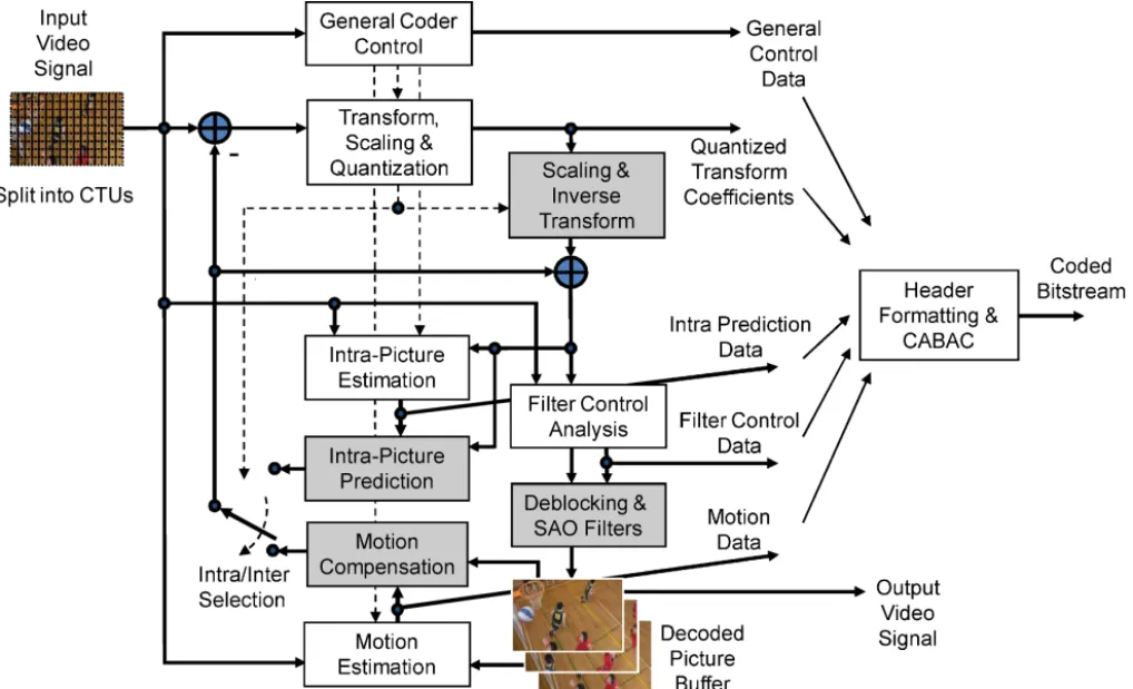
The video coding layer of HEVC employs the same hy-brid approach (inter-/intrapicture prediction and 2-D transform coding) used in all video compression standards since H.261. Fig. 1 depicts the block diagram of a hybrid video encoder, which could create a bitstream conforming to the HEVC standard.

An encoding algorithm producing an HEVC compliant bitstream would typically proceed as follows. Each picture is split into block-shaped regions, with the exact block par-titioning being conveyed to the decoder. The first picture of a video sequence (and the first picture at each clean random access point into a video sequence) is coded using only intrapicture prediction (that uses some prediction of data spatially from region-to-region within the same picture, but has no dependence on other pictures). For all remaining pictures of a sequence or between random access points, interpicture temporally predictive coding modes are typically used for most blocks. The encoding process for interpicture prediction consists of choosing motion data comprising the selected reference picture and motion vector (MV) to be applied for predicting the samples of each block. The encoder and decoder generate identical interpicture prediction signals by applying motion compensation (MC) using the MV and mode decision data, which are transmitted as side information.

The residual signal of the intra- or interpicture prediction, which is the difference between the original block and its pre-diction, is transformed by a linear spatial transform. The trans-form coefficients are then scaled, quantized, entropy coded, and transmitted together with the prediction information.

The encoder duplicates the decoder processing loop (see gray-shaded boxes in Fig. 1) such that both will generate identical predictions for subsequent data. Therefore, the quan-tized transform coefficients are constructed by inverse scaling and are then inverse transformed to duplicate the decoded approximation of the residual signal. The residual is then added to the prediction, and the result of that addition may then be fed into one or two loop filters to smooth out artifacts induced by block-wise processing and quantization. The final picture representation (that is a duplicate of the output of the decoder) is stored in a decoded picture buffer to be used for the prediction of subsequent pictures. In general, the order of encoding or decoding processing of pictures often differs from the order in which they arrive from the source; necessitating a distinction between the decoding order (i.e., bitstream order) and the output order (i.e., display order) for a decoder.

Video material to be encoded by HEVC is generally ex-pected to be input as progressive scan imagery (either due to the source video originating in that format or resulting from deinterlacing prior to encoding). No explicit coding features are present in the HEVC design to support the use of interlaced scanning, as interlaced scanning is no longer used for displays and is becoming substantially less common for distribution. However, a metadata syntax has been provided in HEVC to allow an encoder to indicate that interlace-scanned video has been sent by coding each field (i.e., the even or odd numbered lines of each video frame) of interlaced video as a separate picture or that it has been sent by coding each interlaced frame as an HEVC coded picture. This provides an efficient method of coding interlaced video without burdening decoders with a need to support a special decoding process for it.

In the following, the various features involved in hybrid video coding using HEVC are highlighted as follows.

1) Coding tree units and coding tree block (CTB) structure:

Fig. 1. Typical HEVC video encoder (with decoder modeling elements shaded in light gray).

the macroblock, containing a 16×16 block of luma sam-ples and, in the usual case of 4:2:0 color sampling, two corresponding 8×8 blocks of chroma samples; whereas the analogous structure in HEVC is the coding tree unit (CTU), which has a size selected by the encoder and can be larger than a traditional macroblock. The CTU consists of a luma CTB and the corresponding chroma

CTBs and syntax elements. The size L×L of a luma

CTB can be chosen asL = 16, 32, or 64 samples, with the larger sizes typically enabling better compression. HEVC then supports a partitioning of the CTBs into smaller blocks using a tree structure and quadtree-like signaling [8].

2) Coding units (CUs) and coding blocks (CBs): The quadtree syntax of the CTU specifies the size and positions of its luma and chroma CBs. The root of the quadtree is associated with the CTU. Hence, the size of the luma CTB is the largest supported size for a luma CB. The splitting of a CTU into luma and chroma CBs is signaled jointly. One luma CB and ordinarily two chroma CBs, together with associated syntax, form a coding unit (CU). A CTB may contain only one CU or may be split to form multiple CUs, and each CU has an associated partitioning into prediction units (PUs) and a tree of transform units (TUs).

3) Prediction units and prediction blocks (PBs): The de-cision whether to code a picture area using interpicture or intrapicture prediction is made at the CU level. A PU partitioning structure has its root at the CU level.

Depending on the basic prediction-type decision, the luma and chroma CBs can then be further split in size and predicted from luma and chroma prediction blocks (PBs). HEVC supports variable PB sizes from 64×64 down to 4×4 samples.

4) TUs and transform blocks: The prediction residual is coded using block transforms. A TU tree structure has its root at the CU level. The luma CB residual may be identical to the luma transform block (TB) or may be further split into smaller luma TBs. The same applies to the chroma TBs. Integer basis functions similar to those of a discrete cosine transform (DCT) are defined for the square TB sizes 4×4, 8×8, 16×16, and 32×32. For the 4×4 transform of luma intrapicture prediction residuals, an integer transform derived from a form of discrete sine transform (DST) is alternatively specified.

5) Motion vector signaling: Advanced motion vector pre-diction (AMVP) is used, including derivation of several most probable candidates based on data from adjacent PBs and the reference picture. A merge mode for MV coding can also be used, allowing the inheritance of MVs from temporally or spatially neighboring PBs. Moreover, compared to H.264/MPEG-4 AVC, improved skipped and direct motion inference are also specified. 6) Motion compensation:Quarter-sample precision is used

for the MVs, and 7-tap or 8-tap filters are used for interpolation of fractional-sample positions (compared to six-tap filtering of half-sample positions followed by linear interpolation for quarter-sample positions in

H.264/MPEG-4 AVC). Similar to H.264/MPEG-4 AVC, multiple reference pictures are used. For each PB, either one or two motion vectors can be transmitted, resulting either in unipredictive or bipredictive coding, respec-tively. As in H.264/MPEG-4 AVC, a scaling and offset operation may be applied to the prediction signal(s) in a manner known as weighted prediction.

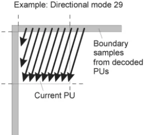
7) Intrapicture prediction: The decoded boundary samples of adjacent blocks are used as reference data for spa-tial prediction in regions where interpicture prediction is not performed. Intrapicture prediction supports 33 directional modes (compared to eight such modes in H.264/MPEG-4 AVC), plus planar (surface fitting) and DC (flat) prediction modes. The selected intrapicture prediction modes are encoded by deriving most probable modes (e.g., prediction directions) based on those of previously decoded neighboring PBs.

8) Quantization control: As in H.264/MPEG-4 AVC, uni-form reconstruction quantization (URQ) is used in HEVC, with quantization scaling matrices supported for the various transform block sizes.

9) Entropy coding:Context adaptive binary arithmetic cod-ing (CABAC) is used for entropy codcod-ing. This is sim-ilar to the CABAC scheme in H.264/MPEG-4 AVC, but has undergone several improvements to improve its throughput speed (especially for parallel-processing architectures) and its compression performance, and to reduce its context memory requirements.

10) In-loop deblocking filtering: A deblocking filter similar to the one used in H.264/MPEG-4 AVC is operated within the interpicture prediction loop. However, the design is simplified in regard to its decision-making and filtering processes, and is made more friendly to parallel processing.

11) Sample adaptive offset (SAO): A nonlinear amplitude mapping is introduced within the interpicture prediction loop after the deblocking filter. Its goal is to better reconstruct the original signal amplitudes by using a look-up table that is described by a few additional parameters that can be determined by histogram analysis at the encoder side.

B. High-Level Syntax Architecture

A number of design aspects new to the HEVC standard improve flexibility for operation over a variety of applications and network environments and improve robustness to data losses. However, the high-level syntax architecture used in the H.264/MPEG-4 AVC standard has generally been retained, including the following features.

1) Parameter set structure:Parameter sets contain informa-tion that can be shared for the decoding of several re-gions of the decoded video. The parameter set structure provides a robust mechanism for conveying data that are essential to the decoding process. The concepts of se-quence and picture parameter sets from H.264/MPEG-4 AVC are augmented by a new video parameter set (VPS) structure.

2) NAL unit syntax structure: Each syntax structure is placed into a logical data packet called a network abstraction layer (NAL) unit. Using the content of a two-byte NAL unit header, it is possible to readily identify the purpose of the associated payload data.

3) Slices: A slice is a data structure that can be decoded independently from other slices of the same picture, in terms of entropy coding, signal prediction, and residual signal reconstruction. A slice can either be an entire picture or a region of a picture. One of the main purposes of slices is resynchronization in the event of data losses. In the case of packetized transmission, the maximum number of payload bits within a slice is typically restricted, and the number of CTUs in the slice is often varied to minimize the packetization overhead while keeping the size of each packet within this bound. 4) Supplemental enhancement information (SEI) and video usability information (VUI) metadata: The syntax in-cludes support for various types of metadata known as SEI and VUI. Such data provide information about the timing of the video pictures, the proper interpretation of the color space used in the video signal, 3-D stereoscopic frame packing information, other display hint informa-tion, and so on.

C. Parallel Decoding Syntax and Modified Slice Structuring

Finally, four new features are introduced in the HEVC stan-dard to enhance the parallel processing capability or modify the structuring of slice data for packetization purposes. Each of them may have benefits in particular application contexts, and it is generally up to the implementer of an encoder or decoder to determine whether and how to take advantage of these features.

1) Tiles: The option to partition a picture into rectangular regions called tiles has been specified. The main pur-pose of tiles is to increase the capability for parallel processing rather than provide error resilience. Tiles are independently decodable regions of a picture that are encoded with some shared header information. Tiles can additionally be used for the purpose of spatial random access to local regions of video pictures. A typical tile configuration of a picture consists of segmenting the picture into rectangular regions with approximately equal numbers of CTUs in each tile. Tiles provide parallelism at a more coarse level of granularity (pic-ture/subpicture), and no sophisticated synchronization of threads is necessary for their use.

2) Wavefront parallel processing: When wavefront parallel processing (WPP) is enabled, a slice is divided into rows of CTUs. The first row is processed in an ordinary way, the second row can begin to be processed after only two CTUs have been processed in the first row, the third row can begin to be processed after only two CTUs have been processed in the second row, and so on. The context models of the entropy coder in each row are inferred from those in the preceding row with a two-CTU processing lag. WPP provides a form of processing parallelism at a rather fine level of

granularity, i.e., within a slice. WPP may often provide better compression performance than tiles (and avoid some visual artifacts that may be induced by using tiles). 3) Dependent slice segments: A structure called a de-pendent slice segment allows data associated with a particular wavefront entry point or tile to be carried in a separate NAL unit, and thus potentially makes that data available to a system for fragmented packetization with lower latency than if it were all coded together in one slice. A dependent slice segment for a wavefront entry point can only be decoded after at least part of the decoding process of another slice segment has been performed. Dependent slice segments are mainly useful in low-delay encoding, where other parallel tools might penalize compression performance.

In the following two sections, a more detailed description of the key features is given.

III. High-Level Syntax

The high-level syntax of HEVC contains numerous elements that have been inherited from the NAL of H.264/MPEG-4 AVC. The NAL provides the ability to map the video coding layer (VCL) data that represent the content of the pictures onto various transport layers, including RTP/IP, ISO MP4, and H.222.0/MPEG-2 Systems, and provides a framework for packet loss resilience. For general concepts of the NAL design such as NAL units, parameter sets, access units, the byte stream format, and packetized formatting, please refer to [9]–[11].

NAL units are classified into VCL and non-VCL NAL units according to whether they contain coded pictures or other associated data, respectively. In the HEVC standard, several VCL NAL unit types identifying categories of pictures for decoder initialization and random-access purposes are included. Table I lists the NAL unit types and their associated meanings and type classes in the HEVC standard.

The following subsections present a description of the new capabilities supported by the high-level syntax.

A. Random Access and Bitstream Splicing Features

The new design supports special features to enable random access and bitstream splicing. In H.264/MPEG-4 AVC, a bitstream must always start with an IDR access unit. An IDR access unit contains an independently coded picture— i.e., a coded picture that can be decoded without decoding any previous pictures in the NAL unit stream. The presence of an IDR access unit indicates that no subsequent picture in the bitstream will require reference to pictures prior to the picture that it contains in order to be decoded. The IDR picture is used within a coding structure known as a closed GOP (in which GOP stands for group of pictures).

The new clean random access (CRA) picture syntax speci-fies the use of an independently coded picture at the location of a random access point (RAP), i.e., a location in a bitstream at which a decoder can begin successfully decoding pictures without needing to decode any pictures that appeared earlier in the bitstream, which supports an efficient temporal coding

TABLE I

NAL Unit Types, Meanings, and Type Classes

Type Meaning Class

0, 1 Slice segment of ordinary trailing picture VCL 2, 3 Slice segment of TSA picture VCL 4, 5 Slice segment of STSA picture VCL 6, 7 Slice segment of RADL picture VCL 8, 9 Slice segment of RASL picture VCL 10–15 Reserved for future use VCL 16–18 Slice segment of BLA picture VCL 19, 20 Slice segment of IDR picture VCL 21 Slice segment of CRA picture VCL 22–31 Reserved for future use VCL 32 Video parameter set (VPS) non-VCL 33 Sequence parameter set (SPS) non-VCL 34 Picture parameter set (PPS) non-VCL 35 Access unit delimiter non-VCL

36 End of sequence non-VCL

37 End of bitstream non-VCL

38 Filler data non-VCL

39, 40 SEI messages non-VCL

41–47 Reserved for future use non-VCL 48–63 Unspecified (available for system use) non-VCL order known as open GOP operation. Good support of random access is critical for enabling channel switching, seek opera-tions, and dynamic streaming services. Some pictures that fol-low a CRA picture in decoding order and precede it in display order may contain interpicture prediction references to pictures that are not available at the decoder. These nondecodable pictures must therefore be discarded by a decoder that starts its decoding process at a CRA point. For this purpose, such nondecodable pictures are identified as random access skipped leading (RASL) pictures. The location of splice points from different original coded bitstreams can be indicated by broken link access (BLA) pictures. A bitstream splicing operation can be performed by simply changing the NAL unit type of a CRA picture in one bitstream to the value that indicates a BLA picture and concatenating the new bitstream at the position of a RAP picture in the other bitstream. A RAP picture may be an IDR, CRA, or BLA picture, and both CRA and BLA pictures may be followed by RASL pictures in the bitstream (depending on the particular value of the NAL unit type used for a BLA picture). Any RASL pictures associated with a BLA picture must always be discarded by the decoder, as they may contain references to pictures that are not actually present in the bitstream due to a splicing operation. The other type of picture that can follow a RAP picture in decoding order and precede it in output order is the random access decodable leading (RADL) picture, which cannot contain references to any pictures that precede the RAP picture in decoding order. RASL and RADL pictures are collectively referred to as leading pictures (LPs). Pictures that follow a RAP picture in both decoding order and output order, which are known as trailing pictures, cannot contain references to LPs for interpicture prediction.

B. Temporal Sublayering Support

Similar to the temporal scalability feature in the H.264/ MPEG-4 AVC scalable video coding (SVC) extension [12],

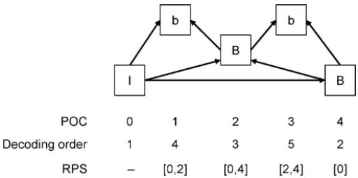
Fig. 2. Example of a temporal prediction structure and the POC values, decoding order, and RPS content for each picture.

HEVC specifies a temporal identifier in the NAL unit header, which indicates a level in a hierarchical temporal prediction structure. This was introduced to achieve temporal scalability without the need to parse parts of the bitstream other than the NAL unit header.

Under certain circumstances, the number of decoded tem-poral sublayers can be adjusted during the decoding process of one coded video sequence. The location of a point in the bitstream at which sublayer switching is possible to begin decoding some higher temporal layers can be indicated by the presence of temporal sublayer access (TSA) pictures and step-wise TSA (STSA) pictures. At the location of a TSA picture, it is possible to switch from decoding a lower temporal sublayer to decoding any higher temporal sublayer, and at the location of an STSA picture, it is possible to switch from decoding a lower temporal sublayer to decoding only one particular higher temporal sublayer (but not the further layers above that, unless they also contain STSA or TSA pictures).

C. Additional Parameter Sets

The VPS has been added as metadata to describe the overall characteristics of coded video sequences, including the dependences between temporal sublayers. The primary purpose of this is to enable the compatible extensibility of the standard in terms of signaling at the systems layer, e.g., when the base layer of a future extended scalable or multiview bitstream would need to be decodable by a legacy decoder, but for which additional information about the bitstream structure that is only relevant for the advanced decoder would be ignored.

D. Reference Picture Sets and Reference Picture Lists

For multiple-reference picture management, a particular set of previously decoded pictures needs to be present in the de-coded picture buffer (DPB) for the decoding of the remainder of the pictures in the bitstream. To identify these pictures, a list of picture order count (POC) identifiers is transmitted in each slice header. The set of retained reference pictures is called the reference picture set (RPS). Fig. 2 shows POC values, decoding order, and RPSs for an example temporal prediction structure.

As in H.264/MPEG-4 AVC, there are two lists that are constructed as lists of pictures in the DPB, and these are called

reference picture list 0 and list 1. An index called a reference picture index is used to identify a particular picture in one of these lists. For uniprediction, a picture can be selected from either of these lists. For biprediction, two pictures are selected—one from each list. When a list contains only one picture, the reference picture index implicitly has the value 0 and does not need to be transmitted in the bitstream.

The high-level syntax for identifying the RPS and estab-lishing the reference picture lists for interpicture prediction is more robust to data losses than in the prior H.264/MPEG-4 AVC design, and is more amenable to such operations as random access and trick mode operation (e.g., fast-forward, smooth rewind, seeking, and adaptive bitstream switching). A key aspect of this improvement is that the syntax is more explicit, rather than depending on inferences from the stored internal state of the decoding process as it decodes the bitstream picture by picture. Moreover, the associated syntax for these aspects of the design is actually simpler than it had been for H.264/MPEG-4 AVC.

IV. HEVC Video Coding Techniques

As in all prior ITU-T and ISO/IEC JTC 1 video coding standards since H.261 [2], the HEVC design follows the classic block-based hybrid video coding approach (as depicted in Fig. 1). The basic source-coding algorithm is a hybrid of interpicture prediction to exploit temporal statistical de-pendences, intrapicture prediction to exploit spatial statistical dependences, and transform coding of the prediction residual signals to further exploit spatial statistical dependences. There is no single coding element in the HEVC design that provides the majority of its significant improvement in compression efficiency in relation to prior video coding standards. It is, rather, a plurality of smaller improvements that add up to the significant gain.

A. Sampled Representation of Pictures

For representing color video signals, HEVC typically uses a tristimulus YCbCr color space with 4:2:0 sampling (although extension to other sampling formats is straightforward, and is planned to be defined in a subsequent version). This separates a color representation into three components called Y, Cb, and Cr. The Y component is also called luma, and represents brightness. The two chroma components Cb and Cr represent the extent to which the color deviates from gray toward blue and red, respectively. Because the human visual system is more sensitive to luma than chroma, the 4:2:0 sampling structure is typically used, in which each chroma component has one fourth of the number of samples of the luma component (half the number of samples in both the horizontal and vertical dimensions). Each sample for each component is typically represented with 8 or 10 b of precision, and the 8-b case is the more typical one. In the remainder of this paper, we focus our attention on the typical use: YCbCr components with 4:2:0 sampling and 8 b per sample for the representation of the encoded input and decoded output video signal.

The video pictures are typically progressively sampled with rectangular picture sizes W×H, where W is the width and

H is the height of the picture in terms of luma samples. Each chroma component array, with 4:2:0 sampling, is then

W/2×H/2. Given such a video signal, the HEVC syntax partitions the pictures further as described follows.

B. Division of the Picture into Coding Tree Units

A picture is partitioned into coding tree units (CTUs), which each contain luma CTBs and chroma CTBs. A luma CTB covers a rectangular picture area ofL×L samples of the luma component and the corresponding chroma CTBs cover each

L/2×L/2 samples of each of the two chroma components. The value ofL may be equal to 16, 32, or 64 as determined by an encoded syntax element specified in the SPS. Compared with the traditional macroblock using a fixed array size of 16×16 luma samples, as used by all previous ITU-T and ISO/IEC JTC 1 video coding standards since H.261 (that was standardized in 1990), HEVC supports variable-size CTBs selected according to needs of encoders in terms of memory and computational requirements. The support of larger CTBs than in previous standards is particularly beneficial when encoding high-resolution video content. The luma CTB and the two chroma CTBs together with the associated syntax form a CTU. The CTU is the basic processing unit used in the standard to specify the decoding process.

C. Division of the CTB into CBs

The blocks specified as luma and chroma CTBs can be directly used as CBs or can be further partitioned into multiple CBs. Partitioning is achieved using tree structures. The tree partitioning in HEVC is generally applied simultaneously to both luma and chroma, although exceptions apply when certain minimum sizes are reached for chroma.

The CTU contains a quadtree syntax that allows for splitting the CBs to a selected appropriate size based on the signal characteristics of the region that is covered by the CTB. The quadtree splitting process can be iterated until the size for a luma CB reaches a minimum allowed luma CB size that is selected by the encoder using syntax in the SPS and is always 8×8 or larger (in units of luma samples).

The boundaries of the picture are defined in units of the minimum allowed luma CB size. As a result, at the right and bottom edges of the picture, some CTUs may cover regions that are partly outside the boundaries of the picture. This condition is detected by the decoder, and the CTU quadtree is implicitly split as necessary to reduce the CB size to the point where the entire CB will fit into the picture.

D. PBs and PUs

The prediction mode for the CU is signaled as being intra or inter, according to whether it uses intrapicture (spatial) prediction or interpicture (temporal) prediction.

When the prediction mode is signaled as intra, the PB size, which is the block size at which the intrapicture prediction mode is established is the same as the CB size for all block sizes except for the smallest CB size that is allowed in the bitstream. For the latter case, a flag is present that indicates whether the CB is split into four PB quadrants that each

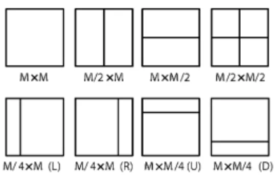
Fig. 3. Modes for splitting a CB into PBs, subject to certain size constraints. For intrapicture-predicted CBs, onlyM ×MandM/2×M/2 are supported. have their own intrapicture prediction mode. The reason for allowing this split is to enable distinct intrapicture prediction mode selections for blocks as small as 4×4 in size. When the luma intrapicture prediction operates with 4×4 blocks, the chroma intrapicture prediction also uses 4×4 blocks (each covering the same picture region as four 4×4 luma blocks). The actual region size at which the intrapicture prediction operates (which is distinct from the PB size, at which the intrapicture prediction mode is established) depends on the residual coding partitioning that is described as follows.

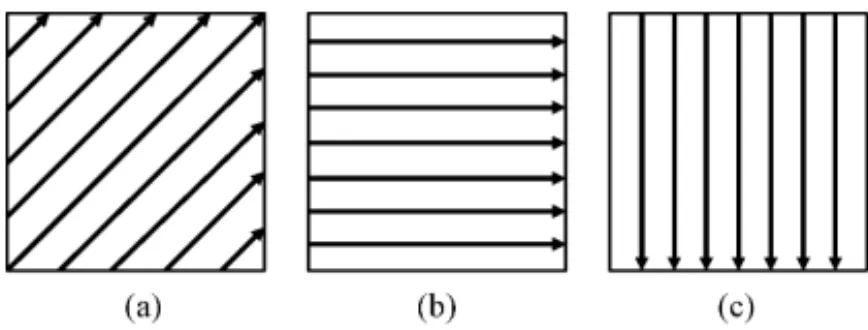
When the prediction mode is signaled as inter, it is specified whether the luma and chroma CBs are split into one, two, or four PBs. The splitting into four PBs is allowed only when the CB size is equal to the minimum allowed CB size, using an equivalent type of splitting as could otherwise be performed at the CB level of the design rather than at the PB level. When a CB is split into four PBs, each PB covers a quadrant of the CB. When a CB is split into two PBs, six types of this splitting are possible. The partitioning possibilities for interpicture-predicted CBs are depicted in Fig. 3. The upper partitions illustrate the cases of not splitting the CB of size

M×M, of splitting the CB into two PBs of size M×M/2 or M/2×M, or splitting it into four PBs of size M/2×M/2. The lower four partition types in Fig. 3 are referred to as asymmetric motion partitioning (AMP), and are only allowed when Mis 16 or larger for luma. One PB of the asymmetric partition has the height or width M/4 and width or height

M, respectively, and the other PB fills the rest of the CB by having a height or width of 3M/4 and width or height M. Each interpicture-predicted PB is assigned one or two motion vectors and reference picture indices. To minimize worst-case memory bandwidth, PBs of luma size 4×4 are not allowed for interpicture prediction, and PBs of luma sizes 4×8 and 8×4 are restricted to unipredictive coding. The interpicture prediction process is further described as follows.

The luma and chroma PBs, together with the associated prediction syntax, form the PU.

E. Tree-Structured Partitioning Into Transform Blocks and Units

For residual coding, a CB can be recursively partitioned into transform blocks (TBs). The partitioning is signaled by a residual quadtree.

Only square CB and TB partitioning is specified, where a block can be recursively split into quadrants, as illustrated in Fig. 4. For a given luma CB of size M×M, a flag signals whether it is split into four blocks of size M/2×M/2. If

Fig. 4. Subdivision of a CTB into CBs [and transform block (TBs)]. Solid lines indicate CB boundaries and dotted lines indicate TB boundaries. (a) CTB with its partitioning. (b) Corresponding quadtree.

further splitting is possible, as signaled by a maximum depth of the residual quadtree indicated in the SPS, each quadrant is assigned a flag that indicates whether it is split into four quadrants. The leaf node blocks resulting from the residual quadtree are the transform blocks that are further processed by transform coding. The encoder indicates the maximum and minimum luma TB sizes that it will use. Splitting is implicit when the CB size is larger than the maximum TB size. Not splitting is implicit when splitting would result in a luma TB size smaller than the indicated minimum. The chroma TB size is half the luma TB size in each dimension, except when the luma TB size is 4×4, in which case a single 4×4 chroma TB is used for the region covered by four 4×4 luma TBs. In the case of intrapicture-predicted CUs, the decoded samples of the nearest-neighboring TBs (within or outside the CB) are used as reference data for intrapicture prediction.

In contrast to previous standards, the HEVC design allows a TB to span across multiple PBs for interpicture-predicted CUs to maximize the potential coding efficiency benefits of the quadtree-structured TB partitioning.

F. Slices and Tiles

Slices are a sequence of CTUs that are processed in the order of a raster scan. A picture may be split into one or several slices as shown in Fig. 5(a) so that a picture is a collection of one or more slices. Slices are self-contained in the sense that, given the availability of the active sequence and picture parameter sets, their syntax elements can be parsed from the bitstream and the values of the samples in the area of the picture that the slice represents can be correctly decoded (except with regard to the effects of in-loop filtering near the edges of the slice) without the use of any data from other slices in the same picture. This means that prediction within the picture (e.g., intrapicture spatial signal prediction or prediction of motion vectors) is not performed across slice boundaries. Some information from other slices may, however, be needed to apply the in-loop filtering across slice boundaries. Each slice can be coded using different coding types as follows.

1) I slice:A slice in which all CUs of the slice are coded using only intrapicture prediction.

2) P slice: In addition to the coding types of an I slice, some CUs of a P slice can also be coded using interpic-ture prediction with at most one motion-compensated prediction signal per PB (i.e., uniprediction). P slices only use reference picture list 0.

3) B slice: In addition to the coding types available in a P slice, some CUs of the B slice can also be coded

Fig. 5. Subdivision of a picture into (a) slices and (b) tiles. (c) Illustration of wavefront parallel processing.

using interpicture prediction with at most two motion-compensated prediction signals per PB (i.e., bipredic-tion). B slices use both reference picture list 0 and list 1. The main purpose of slices is resynchronization after data losses. Furthermore, slices are often restricted to use a maxi-mum number of bits, e.g., for packetized transmission. There-fore, slices may often contain a highly varying number of CTUs per slice in a manner dependent on the activity in the video scene. In addition to slices, HEVC also defines tiles, which are self-contained and independently decodable rectan-gular regions of the picture. The main purpose of tiles is to enable the use of parallel processing architectures for encoding and decoding. Multiple tiles may share header information by being contained in the same slice. Alternatively, a single tile may contain multiple slices. A tile consists of a rectangular arranged group of CTUs (typically, but not necessarily, with all of them containing about the same number of CTUs), as shown in Fig. 5(b).

To assist with the granularity of data packetization, de-pendent slices are additionally defined. Finally, with WPP, a slice is divided into rows of CTUs. The decoding of each row can be begun as soon a few decisions that are needed for prediction and adaptation of the entropy coder have been made in the preceding row. This supports parallel processing of rows of CTUs by using several processing threads in the encoder or decoder (or both). An example is shown in Fig. 5(c). For design simplicity, WPP is not allowed to be used in combination with tiles (although these features could, in principle, work properly together).

G. Intrapicture Prediction

Intrapicture prediction operates according to the TB size, and previously decoded boundary samples from spatially neighboring TBs are used to form the prediction signal. Directional prediction with 33 different directional orientations is defined for (square) TB sizes from 4×4 up to 32×32. The

Fig. 6. Modes and directional orientations for intrapicture prediction. possible prediction directions are shown in Fig. 6. Alterna-tively, planar prediction (assuming an amplitude surface with a horizontal and vertical slope derived from the boundaries) and DC prediction (a flat surface with a value matching the mean value of the boundary samples) can also be used. For chroma, the horizontal, vertical, planar, and DC prediction modes can be explicitly signaled, or the chroma prediction mode can be indicated to be the same as the luma prediction mode (and, as a special case to avoid redundant signaling, when one of the first four choices is indicated and is the same as the luma prediction mode, the Intra₋Angular[34] mode is applied instead).

Each CB can be coded by one of several coding types, depending on the slice type. Similar to H.264/MPEG-4 AVC, intrapicture predictive coding is supported in all slice types. HEVC supports various intrapicture predictive coding methods referred to as Intra−Angular, Intra−Planar, and Intra−DC. The following subsections present a brief further explanation of these and several techniques to be applied in common.

1) PB Partitioning: An intrapicture-predicted CB of size

M×M may have one of two types of PB partitions referred to as PART−2N×2N and PART−N×N, the first of which indicates that the CB is not split and the second indicates that the CB is split into four equal-sized PBs. (Conceptually, in this notation,N = M/2.) However, it is possible to represent the same regions that would be specified by four PBs by using four smaller CBs when the size of the current CB is larger than the minimum CU size. Thus, the HEVC design only allows the partitioning type PART₋N×N to be used when the current CB size is equal to the minimum CU size. This means that the PB size is always equal to the CB size when the CB is coded using an intrapicture prediction mode and the CB size is not equal to the minimum CU size. Although the intrapicture prediction mode is established at the PB level, the actual prediction process operates separately for each TB.

2) Intra−Angular Prediction: Spatial-domain intrapic-ture prediction has previously been successfully used in H.264/MPEG-4 AVC. The intrapicture prediction of HEVC similarly operates in the spatial domain, but is extended significantly—mainly due to the increased size of the TB and an increased number of selectable prediction directions. Compared to the eight prediction directions of H.264/MPEG-4 AVC, HEVC supports a total of 33 prediction directions, denoted as Intra₋Angular[k], wherekis a mode number from

2 to 34. The angles are intentionally designed to provide denser coverage for near-horizontal and near-vertical angles and coarser coverage for near-diagonal angles to reflect the observed statistical prevalence of the angles and the effective-ness of the signal prediction processing.

When using an Intra₋Angular mode, each TB is predicted directionally from spatially neighboring samples that are re-constructed (but not yet filtered by the in-loop filters) before being used for this prediction. For a TB of size N×N, a total of 4N+1 spatially neighboring samples may be used for the prediction, as shown in Fig. 6. When available from preceding decoding operations, samples from lower left TBs can be used for prediction in HEVC in addition to samples from TBs at the left, above, and above right of the current TB.

The prediction process of the Intra₋Angular modes can involve extrapolating samples from the projected reference sample location according to a given directionality. To remove the need for sample-by-sample switching between reference row and column buffers, for Intra₋Angular[k] with k in the range of 2–17, the samples located in the above row are projected as additional samples located in the left column; and withk in the range of 18–34, the samples located at the left column are projected as samples located in the above row. To improve the intrapicture prediction accuracy, the pro-jected reference sample location is computed with 1/32 sample accuracy. Bilinear interpolation is used to obtain the value of the projected reference sample using two closest reference samples located at integer positions.

The prediction process of the Intra₋Angular modes is con-sistent across all block sizes and prediction directions, whereas H.264/MPEG-4 AVC uses different methods for its supported block sizes of 4×4, 8×8, and 16×16. This design consistency is especially desirable since HEVC supports a greater variety of TB sizes and a significantly increased number of prediction directions compared to H.264/MPEG-4 AVC.

3) Intra−Planar and Intra−DC Prediction: In addition to Intra−Angular prediction that targets regions with strong directional edges, HEVC supports two alternative prediction methods, Intra₋Planar and Intra₋DC, for which similar modes were specified in H.264/MPEG-4 AVC. While Intra₋DC pre-diction uses an average value of reference samples for the prediction, average values of two linear predictions using four corner reference samples are used in Intra₋Planar prediction

to prevent discontinuities along the block boundaries. The Intra₋Planar prediction mode is supported at all block sizes in HEVC, while H.264/MPEG-4 AVC supports plane prediction only when the luma PB size is 16×16, and its plane prediction operates somewhat differently from the planar prediction in HEVC.

4) Reference Sample Smoothing: In HEVC, the reference samples used for the intrapicture prediction are sometimes filtered by a three-tap [1 2 1]/4 smoothing filter in a manner similar to what was used for 8×8 intrapicture prediction in H.264/MPEG-4 AVC. HEVC applies smoothing operations more adaptively, according to the directionality, the amount of detected discontinuity, and the block size. As in H.264/MPEG-4 AVC, the smoothing filter is not applied for H.264/MPEG-4×4 blocks. For 8×8 blocks, only the diagonal directions, Intra₋Angular[k] with k = 2, 18, or 34, use the reference sample smoothing. For 16×16 blocks, the reference samples are filtered for most directions except the near-horizontal and near-vertical directions, k in the range of 9–11 and 25–27. For 32×32 blocks, all directions except the exactly horizontal (k = 10) and exactly vertical (k = 26) directions use the smoothing filter, and when the amount of detected discontinuity exceeds a threshold, bilinear interpolation from three neighboring region samples is applied to form a smooth prediction.

The Intra₋Planar mode also uses the smoothing filter when the block size is greater than or equal to 8×8, and the smoothing is not used (or useful) for the Intra₋DC case.

5) Boundary Value Smoothing: To remove discontinuities along block boundaries, in three modes, Intra₋DC (mode 1) and Intra₋Angular[k] with k = 10 or 26 (exactly horizontal or exactly vertical), the boundary samples inside the TB are replaced by filtered values when the TB size is smaller than 32 × 32. For Intra₋DC mode, both the first row and column of samples in the TB are replaced by the output of a two-tap [3 1]/4 filter fed by their original value and the adjacent reference sample. In horizontal (Intra−Angular[10]) prediction, the boundary samples of the first column of the TB are modified such that half of the difference between their neighbored reference sample and the top-left reference sample is added. This makes the prediction signal more smooth when large variations in the vertical direction are present. In vertical (Intra₋Angular[26]) prediction, the same is applied to the first row of samples.

6) Reference Sample Substitution: The neighboring reference samples are not available at the slice or tile boundaries. In addition, when a loss-resilience feature known as constrained intra prediction is enabled, the neighboring reference samples inside any interpicture-predicted PB are also considered not available in order to avoid letting potentially corrupted prior decoded picture data propagate errors into the prediction signal. While only Intra−DC prediction mode is allowed for such cases in H.264/MPEG-4 AVC, HEVC allows the use of other intrapicture prediction modes after substituting the nonavailable reference sample values with the neighboring available reference sample values. 7) Mode Coding: HEVC supports a total of 33 Intra₋Angular prediction modes and Intra₋Planar and Intra₋DC prediction modes for luma prediction for all block

sizes. Due to the increased number of directions, HEVC considers three most probable modes (MPMs) when coding the luma intrapicture prediction mode predictively, rather than the one most probable mode considered in H.264/MPEG-4 AVC. Among the three most probable modes, the first two are ini-tialized by the luma intrapicture prediction modes of the above and left PBs if those PBs are available and are coded using an intrapicture prediction mode. Any unavailable prediction mode is considered to be Intra₋DC. The PB above the luma CTB is always considered to be unavailable in order to avoid the need to store a line buffer of neighboring luma prediction modes.

When the first two most probable modes are not equal, the third most probable mode is set equal to Intra₋Planar, Intra₋DC, or Intra₋Angular[26] (vertical), according to which of these modes, in this order, is not a duplicate of one of the first two modes. When the first two most probable modes are the same, if this first mode has the value Intra₋Planar or Intra₋DC, the second and third most probable modes are assigned as Intra₋Planar, Intra₋DC, or Intra₋Angular[26], according to which of these modes, in this order, are not duplicates. When the first two most probable modes are the same and the first mode has an Intra−Angular value, the second and third most probable modes are chosen as the two angular prediction modes that are closest to the angle (i.e., the value ofk) of the first.

In the case that the current luma prediction mode is one of three MPMs, only the MPM index is transmitted to the decoder. Otherwise, the index of the current luma prediction mode excluding the three MPMs is transmitted to the decoder by using a 5-b fixed length code.

For chroma intrapicture prediction, HEVC allows

the encoder to select one of five modes: Intra₋Planar, Intra₋Angular[26] (vertical), Intra₋Angular[10] (horizontal), Intra₋DC, and Intra₋Derived. The Intra₋Derived mode specifies that the chroma prediction uses the same angular direction as the luma prediction. With this scheme, all angular modes specified for luma in HEVC can, in principle, also be used in the chroma prediction, and a good tradeoff is achieved between prediction accuracy and the signaling overhead. The selected chroma prediction mode is coded directly (without using an MPM prediction mechanism).

H. Interpicture Prediction

1) PB Partitioning: Compared to intrapicture-predicted

CBs, HEVC supports more PB partition shapes for

interpicture-predicted CBs. The partitioning modes of

PART₋2N×2N, PART₋2N×N, and PART₋N×2N indicate the cases when the CB is not split, split into two equal-size PBs horizontally, and split into two equal-size PBs vertically, respectively. PART₋N×N specifies that the CB is split into four equal-size PBs, but this mode is only supported when the CB size is equal to the smallest allowed CB size. In addition, there are four partitioning types that support splitting the CB into two PBs having different sizes: PART₋2N×nU, PART−2N×nD, PART−nL×2N, and PART−nR×2N. These types are known as asymmetric motion partitions.

2) Fractional Sample Interpolation: The samples of the PB for an intrapicture-predicted CB are obtained from those of a

Fig. 7. Integer and fractional sample positions for luma interpolation. corresponding block region in the reference picture identified by a reference picture index, which is at a position displaced by the horizontal and vertical components of the motion vector. Except for the case when the motion vector has an integer value, fractional sample interpolation is used to generate the prediction samples for noninteger sampling positions. As in H.264/MPEG-4 AVC, HEVC supports motion vectors with units of one quarter of the distance between luma samples. For chroma samples, the motion vector accuracy is determined according to the chroma sampling format, which for 4:2:0 sampling results in units of one eighth of the distance between chroma samples.

The fractional sample interpolation for luma samples in HEVC uses separable application of an eight-tap filter for the half-sample positions and a seven-tap filter for the quarter-sample positions. This is in contrast to the process used in H.264/MPEG-4 AVC, which applies a two-stage interpola-tion process by first generating the values of one or two neighboring samples at half-sample positions using six-tap filtering, rounding the intermediate results, and then averaging two values at integer or half-sample positions. HEVC instead uses a single consistent separable interpolation process for generating all fractional positions without intermediate round-ing operations, which improves precision and simplifies the architecture of the fractional sample interpolation. The inter-polation precision is also improved in HEVC by using longer filters, i.e., seven-tap or eight-tap filtering rather than the six-tap filtering used in H.264/MPEG-4 AVC. Using only seven taps rather than the eight used for half-sample positions was sufficient for the quarter-sample interpolation positions since the quarter-sample positions are relatively close to integer-sample positions, so the most distant integer-sample in an eight-tap interpolator would effectively be farther away than in the half-sample case (where the relative distances of the integer-half-sample positions are symmetric). The actual filter tap values of the

TABLE II

Filter Coefficients for Luma Fractional Sample Interpolation

Indexi −3 −2 −1 0 1 2 3 4 hfilter[i] −1 4 −11 40 40 −11 4 1 qfilter[i] −1 4 −10 58 17 −5 1

interpolation filtering kernel were partially derived from DCT basis function equations.

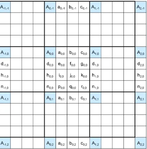
In Fig. 7, the positions labeled with upper-case letters,

Ai,j, represent the available luma samples at integer sample locations, whereas the other positions labeled with lower-case letters represent samples at noninteger sample locations, which need to be generated by interpolation.

The samples labeled a0,j, b0,j, c0,j, d0,0, h0,0, and n0,0 are derived from the samples Ai,j by applying the eight-tap filter for half-sample positions and the seven-tap filter for the quarter-sample positions as follows:

a0,j= (

i=−3..3Ai,jqfilter[i])>>(B−8) b0,j = (

i=−3..4Ai,jhfilter[i])>>(B−8) c0,j= (

i=−2..4Ai,jqfilter[1−i])>>(B−8) d0,0= (

i=−3..3A0,jqfilter[j])>>(B−8) h0,0= (

i=−3..4A0,jhfilter[j])>>(B−8) n0,0= (

j=−2..4A0,jqfilter[1−j])>>(B−8) where the constant B ≥ 8 is the bit depth of the reference samples (and typically B = 8 for most applications) and the filter coefficient values are given in Table II. In these formulas,

>> denotes an arithmetic right shift operation.

The samples labeled e0,0, f0,0, g0,0, i0,0, j0,0, k0,0, p0,0, q0,0, and r0,0 can be derived by applying the corresponding filters to samples located at vertically adjacent a0,j, b0,j and c0,j positions as follows:

e0,0= (

v=−3..3a0,vqfilter[v])>>6 f0,0= (

v=−3..3b0,vqfilter[v])>>6 g0,0= (

v=−3..3c0,vqfilter[v])>>6 i0,0= (

v=−3..4a0,vhfilter[v])>>6 j0,0= (

v=−3..4b0,vhfilter[v])>>6 k0,0= (

v=−3..4c0,vhfilter[v])>>6 p0,0= (

v=−2..4a0,vqfilter[1−v])>>6 q0,0= (

v=−2..4b0,vqfilter[1−v])>>6 r0,0= (

v=−2..4c0,vqfilter[1−v])>>6.

The interpolation filtering is separable when B is equal to 8, so the same values could be computed in this case by applying the vertical filtering before the horizontal filtering. When implemented appropriately, the motion compensation process of HEVC can be performed using only 16-b storage elements (although care must be taken to do this correctly).

It is at this point in the process that weighted pre-diction is applied when selected by the encoder. Whereas H.264/MPEG-4 AVC supported both temporally implicit and explicit weighted prediction, in HEVC only explicit weighted prediction is applied, by scaling and offsetting the prediction with values sent explicitly by the encoder. The bit depth of the prediction is then adjusted to the original bit depth of the reference samples. In the case of uniprediction, the inter-polated (and possibly weighted) prediction value is rounded,

TABLE III

Filter Coefficients for Chroma Fractional Sample Interpolation

Index −1 0 1 2 filter1[i] −2 58 10 −2 filter2[i] −4 54 16 −2 filter3[i] −6 46 28 −4 filter4[i] −4 36 36 −4

right-shifted, and clipped to have the original bit depth. In the case of biprediction, the interpolated (and possibly weighted) prediction values from two PBs are added first, and then rounded, right-shifted, and clipped.

In H.264/MPEG-4 AVC, up to three stages of rounding operations are required to obtain each prediction sample (for samples located at quarter-sample positions). If biprediction is used, the total number of rounding operations is then seven in the worst case. In HEVC, at most two rounding operations are needed to obtain each sample located at the quarter-sample positions, thus five rounding operations are sufficient in the worst case when biprediction is used. Moreover, in the most common usage, where the bit depthBis 8 b, the total number of rounding operations in the worst case is further reduced to 3. Due to the lower number of rounding operations, the accumulated rounding error is decreased and greater flexibility is enabled in regard to the manner of performing the necessary operations in the decoder.

The fractional sample interpolation process for the chroma components is similar to the one for the luma component, except that the number of filter taps is 4 and the fractional accuracy is 1/8 for the usual 4:2:0 chroma format case. HEVC defines a set of four-tap filters for eighth-sample positions, as given in Table III for the case of 4:2:0 chroma format (where, in H.264/MPEG-4 AVC, only two-tap bilinear filtering was applied).

Filter coefficient values denoted as filter1[i], filter2[i], fil-ter3[i], and filter4[i] with i = −1,. . . , 2 are used for inter-polating the 1/8th, 2/8th, 3/8th, and 4/8th fractional positions for the chroma samples, respectively. Using symmetry for the 5/8th, 6/8th, and 7/8th fractional positions, the mirrored values of filter3[1−i], filter2[1−i], and filter1[1−i] with i=−1, . . . , 2 are used, respectively.

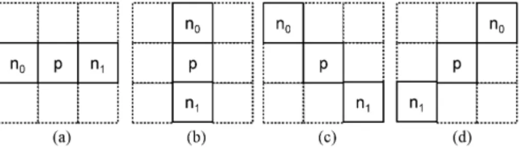
3) Merge Mode: Motion information typically consists of the horizontal and vertical motion vector displacement values, one or two reference picture indices, and, in the case of predic-tion regions in B slices, an identificapredic-tion of which reference picture list is associated with each index. HEVC includes a merge mode to derive the motion information from spatially or temporally neighboring blocks. It is denoted as merge mode since it forms a merged region sharing all motion information. The merge mode is conceptually similar to the direct and skip modes in H.264/MPEG-4 AVC. However, there are two important differences. First, it transmits index information to select one out of several available candidates, in a manner sometimes referred to as a motion vector competition scheme. It also explicitly identifies the reference picture list and ref-erence picture index, whereas the direct mode assumes that these have some predefined values.

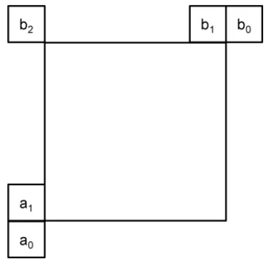
Fig. 8. Positions of spatial candidates of motion information.

The set of possible candidates in the merge mode consists of spatial neighbor candidates, a temporal candidate, and generated candidates. Fig. 8 shows the positions of five spatial candidates. For each candidate position, the availability is checked according to the order {a1, b1, b0, a0, b2}. If the block located at the position is intrapicture predicted or the position is outside of the current slice or tile, it is considered as unavailable.

After validating the spatial candidates, two kinds of redun-dancy are removed. If the candidate position for the current PU would refer to the first PU within the same CU, the position is excluded, as the same merge could be achieved by a CU without splitting into prediction partitions. Furthermore, any redundant entries where candidates have exactly the same motion information are also excluded.

For the temporal candidate, the right bottom position just outside of the collocated PU of the reference picture is used if it is available. Otherwise, the center position is used instead. The way to choose the collocated PU is similar to that of prior standards, but HEVC allows more flexibility by transmitting an index to specify which reference picture list is used for the collocated reference picture.

One issue related to the use of the temporal candidate is the amount of the memory to store the motion information of the reference picture. This is addressed by restricting the granularity for storing the temporal motion candidates to only the resolution of a 16×16 luma grid, even when smaller PB structures are used at the corresponding location in the reference picture. In addition, a PPS-level flag allows the encoder to disable the use of the temporal candidate, which is useful for applications with error-prone transmission.

The maximum number of merge candidates C is specified in the slice header. If the number of merge candidates found (including the temporal candidate) is larger than C, only the first C – 1 spatial candidates and the temporal candidate are retained. Otherwise, if the number of merge candidates identified is less than C, additional candidates are generated until the number is equal toC. This simplifies the parsing and makes it more robust, as the ability to parse the coded data is not dependent on merge candidate availability.

For B slices, additional merge candidates are generated by choosing two existing candidates according to a predefined order for reference picture list 0 and list 1. For example, the first generated candidate uses the first merge candidate for list 0 and the second merge candidate for list 1. HEVC specifies a total of 12 predefined pairs of two in the following order in the already constructed merge candidate list as (0, 1), (1, 0), (0, 2), (2, 0), (1, 2), (2, 1), (0, 3), (3, 0), (1, 3), (3, 1), (2, 3), and (3, 2). Among them, up to five candidates can be included after removing redundant entries.

When the slice is a P slice or the number of merge candidates is still less thanC, zero motion vectors associated with reference indices from zero to the number of reference pictures minus one are used to fill any remaining entries in the merge candidate list.

In HEVC, the skip mode is treated as a special case of the merge mode when all coded block flags are equal to zero. In this specific case, only a skip flag and the corresponding merge index are transmitted to the decoder. The B-direct mode of H.264/MPEG-4 AVC is also replaced by the merge mode, since the merge mode allows all motion information to be derived from the spatial and temporal motion information of the neighboring blocks with residual coding.

4) Motion Vector Prediction for Nonmerge Mode: When an interpicture-predicted CB is not coded in the skip or merge modes, the motion vector is differentially coded using a motion vector predictor. Similar to the merge mode, HEVC allows the encoder to choose the motion vector predictor among multiple predictor candidates. The difference between the predictor and the actual motion vector and the index of the candidate are transmitted to the decoder.

Only two spatial motion candidates are chosen according to the availability among five candidates in Fig. 8. The first spatial motion candidate is chosen from the set of left positions

{a0,a1} and the second one from the set of above positions

{b0,b1,b2}according to their availabilities, while keeping the searching order as indicated in the two sets.

HEVC only allows a much lower number of candidates to be used in the motion vector prediction process for the nonmerge

case, since the encoder can send a coded difference to change the motion vector. Furthermore, the encoder needs to perform motion estimation, which is one of the most computationally expensive operations in the encoder, and complexity is reduced by allowing a small number of candidates.

When the reference index of the neighboring PU is not equal to that of the current PU, a scaled version of the motion vector is used. The neighboring motion vector is scaled according to the temporal distances between the current picture and the reference pictures indicated by the refer-ence indices of the neighboring PU and the current PU, respectively. When two spatial candidates have the same motion vector components, one redundant spatial candidate is excluded.

When the number of motion vector predictors is not equal to two and the use of temporal MV prediction is not explicitly disabled, the temporal MV prediction candidate is included. This means that the temporal candidate is not used at all when two spatial candidates are available. Finally, a zero motion vector is included repeatedly until the number of motion vector prediction candidates is equal to two, which guarantees that the number of motion vector predictors is two. Thus, only a coded flag is necessary to identify which motion vector prediction is used in the case of nonmerge mode.

I. Transform, Scaling, and Quantization

HEVC uses transform coding of the prediction error residual in a similar manner as in prior standards. The residual block is partitioned into multiple square TBs, as described in Section IV-E. The supported transform block sizes are 4×4, 8×8, 16×16, and 32×32.

1) Core Transform: Two-dimensional transforms are com-puted by applying 1-D transforms in the horizontal and vertical directions. The elements of the core transform matrices were derived by approximating scaled DCT basis functions, under considerations such as limiting the necessary dynamic range for transform computation and maximizing the precision and closeness to orthogonality when the matrix entries are speci-fied as integer values.

H=

⎡ ⎢ ⎢ ⎢ ⎢ ⎢ ⎢ ⎢ ⎢ ⎢ ⎢ ⎢ ⎢ ⎢ ⎢ ⎢ ⎢ ⎢ ⎢ ⎢ ⎢ ⎢ ⎢ ⎢ ⎢ ⎢ ⎢ ⎣

64 64 64 64 64 64 64 64 64 64 64 64 64 64 64 64

90 87 80 70 57 43 25 9 −9 −25 −43 −57 −70 −80 −87 90

89 75 50 18 −18 −50 −75 −89 −89 −75 −50 −18 18 50 75 89

87 57 9 −43 −80 −90 −70 −25 25 70 90 80 43 −9 −57 −87

83 36 −36 −83 −83 −36 36 83 83 36 −36 −83 −83 −36 36 83

80 9 −70 −87 −25 57 90 43 −43 −90 −57 25 87 70 −9 −80

75 −18 −89 −50 50 89 18 −75 −75 18 89 50 −50 −89 −18 75

70 −43 −87 9 90 25 −80 −57 57 80 −25 −90 −9 87 43 −70

64 −64 −64 64 64 −64 −64 64 64 −64 −64 64 64 −64 −64 64

57 −80 −25 90 −9 −87 43 70 −70 −43 87 9 −90 25 80 −57

50 −89 18 75 −75 −18 89 −50 −50 89 −18 −75 75 18 −89 50

43 −90 57 25 −87 70 9 −80 80 −9 −70 87 −25 −57 90 −43

36 −83 83 −36 −36 83 −83 36 36 −83 83 −36 −36 83 −83 36

25 −70 90 −80 43 9 −57 87 −87 57 −9 −43 80 −90 70 −25

18 −50 75 −89 89 −75 50 −18 −18 50 −75 89 −89 75 −50 18

9 −25 43 −57 70 −80 87 −90 90 −87 80 −70 57 −43 25 −9

⎤ ⎥ ⎥ ⎥ ⎥ ⎥ ⎥ ⎥ ⎥ ⎥ ⎥ ⎥ ⎥ ⎥ ⎥ ⎥ ⎥ ⎥ ⎥ ⎥ ⎥ ⎥ ⎥ ⎥ ⎥ ⎥ ⎥ ⎦