Improved Controller Design for Turbocharged
Diesel Engine
Magdi S. Mahmoud Member, IAENG
Abstract—Turbocharged diesel engines are now being used in every automobile by a lot of automobile manufacturing companies. A turbocharged diesel engine (TDE) equipped with variable geometry turbocharger and exchange gas recirculation is explained in detail. A linear turbocharged diesel engine model is presented and its control techniques are explained in detail. Controllers are designed using the linear-quadratic regulator (LQR), linear-quadratic Gaussian regulator (LQGR),H2,H∞,
and mixed H2/H∞. A comparison is made among these
controllers based on the ensuing results of Matlab simulation.
Index Terms—Optimal control, LQR, LQG, H2, H∞,
tur-bocharged diesel engines
I. INTRODUCTION
I
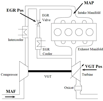
N recent years more stringent requirements on perfor-mance, fuel conservation and low emissions have paved way for increased complicated engine performance. Strate-gies like exhaust gas recirculation and turbocharging have been devised to cope up with the requirements. These give us a great bit of freedom to control the behavior of the engine. Previous practices used these in a suboptimal way since the devices used to control these features affect many different parts of the engine through the cross-couplings in the system. The development of an optimal coordinated strategy often takes more time than available in a production cycle. In order to fully extract the potential of these devices we consider this as a multivariable control problem. A multivariable approach to this will yield a better performance. Turbochargers mainly find their applications in racing cars,automobiles, aircrafts and gas turbines. Diesel (compression ignition) engines hold a significant advantage over spark ignited (gasoline) engines in fuel economy. Moreover, diesel engines have lower feed-gas emissions of the regulated exhaust feed-gases, but the after-treatment devices for diesel engines are far less efficient than the conventional three way catalysts for spark ignition engines.In this paper, the plant to be controlled is a turbocharged passenger car diesel engine equipped with exhaust gas recir-culation and a variable geometry turbine as shown in Fig. 1. Turbocharger increases the power density of the engine by forcing air into the cylinders, which allows injection of additional fuel without reaching the smoke limit. The turbine, which is driven by the energy in the exhaust gas, has a variable geometry that allows the adaptation of the turbine efficiency based on the engine operating point. The second feedback path from the exhaust to the intake manifold is
Manuscript received January, 2012. This work is supported by the deanship for scientific research (DSR) at King Fahd University for Petroleum and Minerals (KFUPM) through research group project RG1105-1.
Magdi S. Mahmoud is with the Systems Engineering Department, King Fahd University for Petroleum and Minerals (KFUPM), PO Box 5067, Dhahran 31261, Saudi Arabia. (Phone: 00-966-54201-9258; Fax: 00-9663-860-2965; e-mail: msmahmoud@ kfupm.edu.sa).
[image:1.595.323.527.248.448.2]due to the EGR, which is controlled by the EGR valve. The recirculated exhaust gas replaces oxygen in the inlet charge, thereby reducing the temperature profile of the combustion and hence the emissions of oxides and nitrogen. Modern
Figure 1: Schematic diagram of the TDE model
diesel engines are typically equipped with the VGT and EGR and both introduce feedback loops from exhaust to intake manifold. The recirculated exhaust gas is cooled down in the EGR cooler and its mass flow is controlled via the EGR valve. Both the EGR valve and the VGT are pneumatically actuated and fitted with position sensors. An intercooler reduces the temperature of the compressed air coming from the compressor. In addition to the standard production type sensors, for mass air flow (MAF) and manifold absolute pres-sure (MAP), the engine is equipped with various temperature and pressure sensors as well as with a turbocharger speed and inline shaft torque sensor. Exhaust gas recirculation (EGR) combined with the variable geometry turbocharging provides an important avenue for NOx emission reduction.
The objective of this paper is to proved improved methods for the controller design of a turbocharged diesel engine. The methods include quadratic regulator (LQR), linear-quadratic Gaussian regulator (LQGR),H2, H∞, and mixed
H2/H∞, which are proved in convenient computable form.
II. STATE-SPACEMODEL
In what follows, we consider a typical turbocharger con-sisting of an exhaust gas driven turbine that, by means of a mechanical shaft, is able to transfer its kinetic energy to the compressor impeller. The impeller imparts this energy to the air, which is turned into density increase in the compressor diffuser. The variable geometry turbocharging is accomplished by a turbine that has a system of movable guide vanes located on the turbine stator. By adjusting the guide vanes, the exhaust gas energy to the turbocharger can be regulated, thus controlling the compressor mass airflow and exhaust manifold pressure. The variable geometry tur-bocharger(VGT) actuator is typically used to control the intake manifold absolute pressure(MAP) and the EGR valve controls the mass air flow (MAF) into the engine. Both the EGR and VGT paths are driven by the exhaust gas and hence constitute an inherently multivariable control problem. Recall that the effect of the EGR and VGT actuators is coupled through the pressure in the exhaust manifold, therefore a co-ordinated approach will yield a better performance than the control strategies using SISO techniques.
An appropriate linearized model that can be conveniently cast into the format
˙
x(t) = Ax(t) +Bu(t) + Γw(t)
z(t) = Gx(t) +Du(t) + Φw(t)
y(t) = Cx(t) + Ψw(t) (1) where x(t) ∈ ℜn, u(t) ∈ ℜm, y(t) ∈ ℜp, z(t) ∈ ℜq andw(t) ∈ ℜq are the state, the control input, the measured output, the controlled output and the external disturbance vectors. The matrices A, B, C, G, D, F, Φ, Ψare real constants, the numerical values of which are given in the simulation section. In system (1), the states components are
mx = mass at the exhaust manifold, px = pressure at the exhaust manifold, mi =mass at the intake manifold,pi = pressure at the exhaust manifold, Nt = turbocharger shaft speed andWci=compressor mass flow. The system inputs are u1 =exhaust gas recirculation (EGR) actuator position
and u2 = variable geometry turbocharger (VGT) actuator
(vanes) position, whereas the system outputs which arey1=
intake manifold absolute pressure (MAP) and y2 = intake
mass air flow (MAF).
III. LQR DESIGN
Here, the associated quadratic cost function is
J =
Z ∞
0
[yt(t)Qy(t) +ut(t)Ru(t)]dt (2) where0<Q, 0<R are output error and control weighting matrices, which are selected in the course of simulation by observing several sets of criteria of the closed loop-system. In what follows, we present an LMI-based formulation to the LQ control of system (1) while minimizing the quadratic cost (2). We proceed to determine a linear optimal state-feedback control u=Lx that achieves this goal. Assume that V(x)
has the formV(x) =xtK
+x, K+ > 0and satisfies ˙
V(x)≤ −[xtCtQCx+utRu] (3)
Then, the linear system controlled by u is asymptotically stable and J∞ ≤ V(xo). With u=Lx, inequality (3) is equivalently expressed as
xt[K+(A+BL) + (A+BL)tK+]t x
≤ −xt[CtQC+LtRL]x (4) From (4), it is evident that (3) is satisfied if there existsL
andK+ such that
K+(A+BL) + (A+BL)tK+t +
[CtQC+LtRL] ≤ 0 (5) Morover, instead of directly minimizing the costxt
oK+xo, we proceed to minimize its upper bound. Therefore, we assume that there existsγ+>0 such that
xt
oK+xo ≤ γ+ (6)
In effect, the linear optimal control problem under consider-ation for givenγ+ can be cast into the format
min
γ+,K+,L
γ+ subject to(5)−(6) (7)
To convexify the above problem, we first express (5) as
Φ =K+(A+BL) + (A+BL)tK+t Π =
Φ Ct Lt • −Q−1 0
• • −R−1
≤ 0 (8)
Pre- and post-multiply (8) by diag{K−1
∗ , I, I} and using
Y =K−1
+ , S =LK
−1
+ it follows that (8) is equivalent to
(AY +BS) + (AY +BS)t Y Ct Y Lt
• −R−1
0
• • −Q−1
≤0(9)
Additionally, inequality (6) can be expressed as
γ+ xto
• K−1 +
≥0⇐⇒
γ+ xto
• Y
≥0 (10)
The minimization problem (7) is cast into the form
min
γ+,Y,S
γ+ subject to(9)−(10) (11)
When a feasible solution of problem (11) is attained, then we getL = S Y−1, K
+=Y−1
IV. H2ANDH∞DESIGN
We now direct attention to alternative techniques for computing the state-feedback controller u = Lx, . The closed-loop system is described by
˙
xs(t) = Asxs(t) + Γw(t)
z(t) = Gsxs(t) + Φw(t) (12)
As = A+BL, Gs=G+DL (13) Designing anH2 controller is approached via convex
analy-sis. Suppose a Lyapunov function for the closed-loop system (12) is selected as
V(xs) =xtsPxs(t), 0<Pt=P ∈ ℜn
×n (14)
Along the solutions of the closed-loop system (12) with
w(t)≡0, we obtain
˙
V(xs) = xst PAs+AtsP
From the Lyapunov theorem, the closed-loop system (12) is internally asymptotically stable if
AtsP+PAs < 0 (16) is satisfied. The objective of this paper is to develop LMI-based characterization of the two optimization problems
A) The H2-norm optimization in which it is required
to find the state-feedback gain L that ensures the stability of closed-loop system (12) and keeps the H2-norm of the
transfer functionTzw(s) fromw tozas small as possible.
B) TheH∞-norm optimization in which it is required to find the state-feedback gain L that ensures the stability of closed-loop system (12) and keeps the||z||2 < γ||w||2for
a prescribed attenuation level γ >0.
A. H2 design
Provided matrix As is Hurwitz for given L with Φ ≡
0, Ψ ≡ 0, the square of the H2-norm of the transfer
funstion Hzw(s) can be expressed in terms of the solution of a Lyapunov equation (controllability Grammian) such that the corresponding minimization problem with respect L is given by
min
T r[Ct
sPsCs] : AsPs + PsAts+ ΓΓt = 0
(17)
where T r[.] denotes the trace operator. Since Ps < P for any P satisfying
AsP + PAts+ ΓΓt < 0 (18) it is readily verified that ||Hzw(s)||22 = T r[CstPCs] < ν if and only if there exists P > 0 satisfying (18) and
T r[Ct
sPCs] < ν. Introducing an auxiliary parameter W, and in line of [7] the following analysis result is obtained: Theorem 4.1: : Matrix As is stable and ||Hzw(s)||22< ν
for a prescribed ν if and only if there exist matricesPb, W such that
T r(W) < ν, (19)
At
sPb+PbAs PbΓ
• −I
< 0
b P Ct
s
• W
>0, (20) The main design result is summarized by the following theorem:
Theorem 4.2: : System (12)-(13) is stable with ||Hzw(s)||22 < ν for a prescribed ν if and only if
there exist matrices 0<X, 0<Y and W such that
T r(W) < ν, (21)
AX +XAt+BY+YtBt Γ
• −I
< 0 (22)
X XGt+YtDt
• W
>0 (23) Moreover, the controller gain is L=YX−1
Proof: A congruent transformation [7], [8], [9] via
diag[X I], X =Pb−1 on (20) yields (23).
B. H∞ design
In what follows, we consider theH∞-norm optimization problem. It follows from robust control theory [10] that the solution of this problem corresponds to determining the controller parameters that guarantees the feasibility of
˙
V(xs) +ztz − γ2wtw<0 (24) The design result is summarized by the following theorem:
Theorem 4.3: : System (12) is asymptotically stable with
γ-disturbance attenuation if there exist matrices0<X, 0<
Y, and scalarγ >0 satisfying the following LMI
Πo Γ Πc • −γ2I Φt
• • −I
< 0 (25)
Πo=AX+XAt+BY+YtBt
Πc=XGt+YtDt (26) Moreover, the controller gain isL=YX−1
Proof: With the aid of (15), we express inequality (24) in the form
xts[PAs+AtsP]xs+ [Csxs+ Φw]t[Csxs+ Φw] +
2xtsPΓ−γ2
wtw < 0 (27)
Inequality (27), by Schur complements, is equivalent to
PAs+AtsP PBs Cst • −γ2I Dt s
• • −I
< 0 (28)
for any[xs, w]6= 0. Applying the congruent transformation
diag[X I], X = Pb−1 to (28) and using LX = Y, we
readily obtain LMI (25) subject to (26 ), which concludes the proof.
C. MixedH2-H∞ synthesis
Considering system (1), the mixed H2-H∞ synthesis problem deals with the problem of finding the state-feedback controller which minimizes the H2 norm of the transfer
function Tzw(s) and subject to the H∞-norm constrained by the boundγ.
V. LQGR DESIGN
In this case, we represent the TDE system by the model
˙
x(t) = Ax(t) +Bu(t) + Γd(t)
z(t) = Gx(t) +Du(t)
y(t) = Cx(t) +n(t) (29) where d and n are zero-mean Gaussian noise processes (uncorrelated from each other) with power spectrumsQ, R,
respectively. Building on the LQR design, we consider that the state-feedback controlleru=Lxis available and proceed to construct an LQG estimator of the form
˙ˆ
x(t) = [A−KC]ˆx(t) +Bu(t) +Ky (30) whereKis the Kalman estimator gain. In terms of the error e(t) =x(t)−xˆ(t),we have
˙
e = Ae+ Γd−Kn (31) The optimal gain matrixKis given byK=SCtR−1where 0<S=Stis the solution to the following Algebraic Riccati Equation (ARE)
AS+SAt+ ΓQΓt−SCtR−1
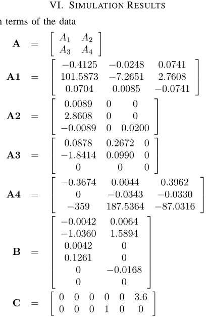
VI. SIMULATIONRESULTS
In terms of the data
A =
A1 A2
A3 A4
A1 =
−0.4125 −0.0248 0.0741 101.5873 −7.2651 2.7608 0.0704 0.0085 −0.0741
A2 =
0.0089 0 0 2.8608 0 0
−0.0089 0 0.0200
A3 =
0.0878 0.2672 0
−1.8414 0.0990 0
0 0 0
A4 =
−0.3674 0.0044 0.3962 0 −0.0343 −0.0330
−359 187.5364 −87.0316
B =
−0.0042 0.0064
−1.0360 1.5894 0.0042 0 0.1261 0
0 −0.0168
0 0
C =
0 0 0 0 0 3.6 0 0 0 1 0 0
Numerical simulation of the controll designs using the linear-quadratic regulator (LQR), linear-linear-quadratic Gaussian regula-tor (LQGR),H2,H∞, and mixedH2/H∞, are summarized
in terms of the feedback gains and the associated bounds:
Lℓqr=
−0.8195 −0.1731 −0.1973 1.1521 −0.9907 −0.0028 5.14277 0.3250 0.3654 0.7437 0.1943 0.0025
,
||Lℓqr||= 5.2748, γ+ = 6.3472
L2 =
−
1.6713 −0.5447 −0.3060 3.7550 −2.8728 −0.0109 13.59667 1.0298 0.6755 2.3428 0.2124 0.0076
, L2 = 13.9038, ν= 9.1428
L∞=
−0.6200 −0.1231 −0.1584 0.8140 −0.7184 −0.0019 3.7531 0.23097 0.28567 0.5287 0.1598 0.0018
,
||L∞||= 3.8540, γ= 2.3814
L2−∞=
−
0.1796 −0.0317 −0.0526 0.2068 −0.1942 −0.0005 1.0156 0.0594 0.0900 0.1362 0.0550 0.0005
,
||L2−∞||= 1.0463, ν= 2.3619, γ= 0.9327
Lℓqgr=
−
0.341 −0.0628 −0.0950 0.4114 −0.3772 −0.0009 1.9763 0.1176 0.1655 0.2696 0.0982 0.0009
,
||Lℓqgr||= 2.0334, γ+ = 6.3472
The numerical clearly suggests that the control design based on the mixed H2/H∞ yields the best compromize. However, it requires, exessive computations compared with LQR, H2andH∞. The corresponding state trajectories are
plotted in Figs. 2-7.
Figure 2: Response of state 1
[image:4.595.63.269.57.371.2]Figure 3: Response of state 2
Figure 4: Response of state 3
[image:4.595.63.273.633.765.2]Figure 5: Response of state 4
Figure 7: Response of state 6
Acknowledgment
This research work is supported by the deanship for scientific research (DSR) at KFUPM through research group project
RG1105-1.
VII. CONCLUSIONS
This paper has
• presented a linear turbocharged diesel engine model and explained its control requirements.
• provided control design methods based on the theories of LQR, LQGR, H2, H∞, and mixed H2/H∞. The
methods are cast into convenient computing forms.
• made a comparison among the designed controllers based on Matlab simulation of the closed-loop system results.
Judged by how much the exhaust mass and exhaust pressure is reduced to reduce the emission from the engine, it has been concluded that mixed H2/H∞ yields the best performance as it has the least norm of the gain matrix. This tends to maximize the pressure at the intake which in turn gives the boost to the engine.
REFERENCES
[1] Merten Jung, Keith Glover, Urs Christen, ”Comparison of uncertainty parameterisations for robust control of turbocharged diesel engines”,
Control Engineering Practice, vol. 13, no. 1, 2005, pp. 15–25.
[2] Friedrich, I.; Chia-Shang Liu; Oehlerking, D.; , ”Coordinated EGR-rate model-based controls of turbocharged diesel engines via an intake throttle and an EGR valve,” IEEE Conference on Vehicle Power and
Propulsion, VPPC ’09, 7-10 Sept. 2009, pp. 340–347.
[3] Cooper, A.R.; Morrow, D.J.; Chambers, K.D.R.; , ”A turbocharged diesel generator set model,” Proc. of the 44th Inte. Universities Power
Engineering Conference (UPEC), 1–4 Sept. 2009, pp. 1–5.
[4] Fredriksson, J.; Egardt, B.; , ”Backstepping control with local LQ performance applied to a turbocharged diesel engine,” Proc. of the 40th
IEEE Conference on Decision and Control, vol. 1, 2001, pp. 111–116.
[5] Wang Haiyan; , ”Control oriented dynamic modeling of a turbocharged diesel engine,” Intelligent Systems Design and Applications, Sixth Int.
Conference on ISDA ’06, vol.2, 16–18 Oct. 2006, pp.1 42–145.
[6] Mario A. Rotea, ”The generalizedH2 control problem”, Automatica, vol. 29, no. 2, 1993, pp. 373–385.
[7] M. S. Mahmoud, ”ResilientL2− L∞Filtering of Polytopic Systems with State-Delays”, IET Control Theory and Applications, vol. 1, no. 1, 2007, pp. 141–154.
[8] M. S. Mahmoud and A. Y. Al-Rayyah, ”Efficient Parameterization to Stability and Feedback Synthesis of Linear Time-Delay Systems”, IET
Control Theory and Applications, vol. 3, no. 8, 2009, pp. 1107–1118.
[9] M. S. Mahmoud and Yuanqing Xia, ”Robust Filter Design for Piecewise Discrete-Time Systems with Time-Varying Delays”,, Int. J. Robust and
Nonlinear Control, vol. 20, 2010, pp. pp. 540–560.