Fast and Robust Joint Models for Biomedical Event Extraction

Proceedings of the 2011 Conference on Empirical Methods in Natural Language Processing, pages 1–12,

Fast and Robust Joint Models for Biomedical Event Extraction

Sebastian Riedel Andrew McCallum

Department of Computer Science University of Massachusetts, Amherst {riedel,mccallum}@cs.umass.edu

Abstract

Extracting biomedical events from literature has attracted much recent attention. The best-performing systems so far have been pipelines of simple subtask-specific local classifiers. A natural drawback of such approaches are cas-cading errors introduced in early stages of the pipeline. We present three joint models of increasing complexity designed to overcome this problem. The first model performs joint trigger and argument extraction, and lends it-self to a simple, efficient and exact infer-ence algorithm. The second model captures correlations between events, while the third model ensures consistency between arguments of the same event. Inference in these models is kept tractable through dual decomposition. The first two models outperform the previous best joint approaches and are very competi-tive with respect to the current state-of-the-art. The third model yields the best results re-ported so far on the BioNLP 2009 shared task, the BioNLP 2011 Genia task and the BioNLP 2011 Infectious Diseases task.

1 Introduction

Whenever we advance our scientific understanding of the world, we seek to publish our findings. The result is a vast and ever-expanding body of natural language text that is becoming increasingly difficult to leverage. This is particularly true in the context of life sciences, where large quantities of biomedi-cal articles are published on a daily basis. To sup-port tasks such data mining, search and visualiza-tion, there is a clear need for structured representa-tions of the knowledge these articles convey. This is

indicated by a large number of public databases with content ranging from simple protein-protein interac-tions to complex pathways. To increase coverage of such databases, and to keep up with the rate of pub-lishing, we need toautomaticallyextract structured representations from biomedical text—a process of-ten referred to as biomedical text mining.

One major focus of biomedical text mining has been the extraction of named entities, such genes or gene products, and of flat binary relations be-tween such entities, such as protein-protein interac-tions. However, in recent years there has also been an increasing interest in the extraction of biomedi-caleventsand their causal relations. This gave rise to the BioNLP 2009 and 2011 shared tasks which challenged participants to gather such events from biomedical text (Kim et al., 2009; Kim et al., 2011). Notably, these events can be complex and recursive: they may have several arguments, and some of the arguments may be events themselves.

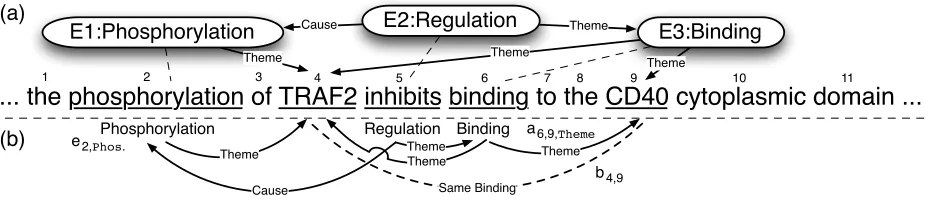
... the phosphorylation of TRAF2 inhibits binding to the CD40 cytoplasmic domain ...

Theme

Cause Theme

Theme

Theme

Regulation Binding Phosphorylation

Theme

Cause

Theme

Theme Theme Same Binding

1 2 3 4 5 6 7 8 9 10 11

b_4,9 e2,Phos.

a_6,9,Theme

(a)

(b)

Figure 1: (a) sentence with target event structure to extract; (b) projection to a set of labelled graph over tokens.

it concerns. Current systems attempt to tackle this problem by passing several candidates to the next stage. However, this tends to increase the false pos-itive rate. In fact, Miwa et al. (2010c) observe that 30% of their errors stem from this type of ad-hoc module communication.

Joint models have been proposed to overcome this problem (Poon and Vanderwende, 2010; Riedel et al., 2009). However, besides not being as accurate as their pipelined competitors, mostly because they do not yet exploit the rich set of features used by Miwa et al. (2010b) and Björne et al. (2009), they also suffer from the complexity of inference. For example, to remain tractable, the best joint system so far (Poon and Vanderwende, 2010) works with a simplified representation of the problem in which certain features are harder to capture, employs local search without certificates of optimality, and further-more requires a 32-core cluster for quick train-test cycles. Existing joint models also rely on heuristics when it comes to deciding which arguments share the same event. Contrast this with the best current pipeline (Miwa et al., 2010c; Miwa et al., 2010b) which uses a classifier for this task.

We present a family of event extraction mod-els that address the aforementioned problems. The first model jointly predicts triggers and arguments. Notably, the highest scoring event structure under this model can be found efficiently inO(mn)time

where m is the number of trigger candidates, and

n the number of argument candidates. This is

only slightly slower than theO(m0n) runtime of a

pipeline, where m0 is the number of trigger candi-dates as filtered by the first stage. We achieve these guarantees through a novel algorithm that jointly picks best trigger label and arguments on a per-token basis. Remarkably, it takes roughly as much time to

train this model on one core as the model of Poon and Vanderwende (2010) on 32 cores, and leads to better results.

The second model enforces additional constraints that ensure consistency between events in hierarchi-cal regulation structures. While inference in this model is more complicated, we show how dual de-composition (Komodakis et al., 2007; Rush et al., 2010) can be used to efficiently find exact solutions for a large fraction of problems.

Our third model includes the first two, and explic-itly captures which arguments are part in the same event—the third stage of existing pipelines. Due to a complex coupling between this model and the first two, inference here requires a projected version of the sub-gradient technique demonstrated by Rush et al. (2010).

When evaluated on the BioNLP 2009 shared task, the first two models outperform the previous best joint approaches and are competitive when com-pared to current state-of-the-art. With 57.4 F1 on the test set, the third model yields the best results reported so far with a 1.1 F1 margin to the results of Miwa et al. (2010b). For the BioNLP 2011 Ge-nia task 1 and the BioNLP 2011 Infectious Diseases task, Model 3 yields the second-best and best results reported so far. The second-best results are achieved with Model 3 as is (Riedel and McCallum, 2011), the best results when using Stanford event predic-tions as input features (Riedel et al., 2011). The margins between Model 3 and the best runner-ups range from 1.9 F1 to 2.8 F1.

Grb2 can be coimmunoprecipitated with Sos1 and Sos2

Binding Binding

Theme Theme Theme _Theme

Theme Theme Theme

1 2 3 4 5 6 7 8

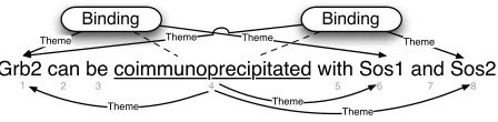
Figure 2: Two binding events with identical trigger. The projection graph does not change even if both events are merged.

2 Biomedical Event Extraction

By bio-molecular event we mean a change of state of one or more bio-molecules. Our task is to extract structured information about such events from nat-ural language text. More concretely, let us consider part (a) of figure 1. We see a snippet of text from a biomedical abstract, and the three events that can be extracted from it. We will use these to characterize the types of events we ought to extract, as defined by the 2009 BioNLP shared task. Note that for the shared task, protein mentions are given by the task organizers and hence do not need to be extracted.

The event E1 in the figure refers to a Phosphory-lation of the TRAF2 protein. It is an instance of a set of simple eventsthat describe changes to a sin-gle gene or gene product. Other members of this set are:Expression,Transcription,Localization, and

Catabolism. Each of these events has to have exactly onetheme, the protein of which a state change is de-scribed. A labelled edge in figure 1a) shows that TRAF2 is the theme of E1.

Event E3 is a Binding of TRAF2 and CD40. Binding events are particular in that they may have more than one theme, as there can be several bio-molecules associated in a binding structure. This is in fact the case for E3.

In the top-center of figure 1a) we see the Regu-lationevent E2. Such events describe regulatory or causal relations between events. Other instances of this type of events are:Positive Regulationand Neg-ative Regulation. Regulations have to have exactly one theme; this theme can a be protein or, as in our case, another event. Regulations may also have zero or one cause arguments that denote events or pro-teins which trigger the regulation.

In the BioNLP shared task, we are also asked to find atrigger (or clue) token for each event. This token grounds the event in text and allows users to

quickly validate extracted events. For example, the trigger for event E2 is “inhibit”, as indicated by a dashed line.

2.1 Event Projection

To formulate the search for event structures of the form shown in figure 1a) as an optimization prob-lem, it will be convenient to represent them through a set of binary variables. We introduce such a rep-resentation, inspired by previous work (Riedel et al., 2009; Björne et al., 2009) and based on a projection of events to a graph structure over tokens, as seen figure 1b).

Consider sentencexand a set ofcandidate trig-gertokens, denoted by Trig(x). We label each

can-didate i with the event type it is a trigger for, or None if it is not a trigger. This decision is rep-resented through a set of binary variablesei,t, one

for each possible event type t. In our example we havee6,Binding = 1. The set of possible event types

will be denoted asT, the regulation event types as TRegdef={PosReg,NegReg,Reg}and its complement

asT¬reg=def T \ TReg.

For each candidate triggeriwe consider the

argu-ments of all events that have ias trigger. Each

ar-gumentawill either be an event itself, or a protein. For events we add a labelled edge betweeniand the

triggerjofa. For proteins we add an edge between iand the syntactic headjof the protein mention. In both cases we label the edgei → j with the role

of the argumenta. The edge is represented through

a binary variable ai,j,r, where r ∈ R is the

argu-ment role and R def= _{Theme,Cause,None_}. The role None is active whenever no Theme or Cause role is present. In our example we get, among oth-ers,a2,4,Theme = 1.

So far our representation is equivalent to map-pings in previous work (Riedel et al., 2009; Björne et al., 2009) and hence shares their main shortcoming: we cannot differentiate between two (or more) bind-ing events with the same trigger but different argu-ments, or one binding event with several arguments. Consider, for example, the arguments of trigger 6 in figure 1b) that are all subsumed in a single event. By contrast, the arguments of trigger 4 shown in figure 2 are split between two events.

through ad-hoc rules (Björne et al., 2009) or with a post-processing classifier (Miwa et al., 2010c). We propose to augment the graph representation through edges between pairs of proteins that are themes in the same binding event. For two protein tokensp andq we represent this edge through the

binary variable bp,q. Hence, in figure 1b) we have b4,9 = 1, whereas for figure 2 we getb1,6 =b1,8 = 1

but b6,8 = 0. By explicitly modeling such

“sib-ling” edges we not only minimize the need for post-processing. We can also improve attachment deci-sions akin to second order models in dependency parsing (McDonald and Pereira, 2006). Note that while merely introducing such variables is easy, en-forcing consistency between them and the ei,t and ai,j,r variables is not. We address this in section

3.3.1.

Reconstruction of events from solutions(e,a,b)

can be done almost exactly as described by Björne et al. (2009). However, while they group binding arguments according to ad-hoc rules based on de-pendency paths from trigger to argument, we simply query the variablesbp,q.

To simplify our exposition we introduce addi-tional notation. We denote the set of protein head tokens with Prot(x); the set of a possible targets

for outgoing edges from a trigger is Cand(x) =def

Trig(x) _∪ Prot(x). We will often omit the

mains of indices and instead assign them a fixed do-main in advance: i, l _∈ Trig(x), j, k _∈ Cand(x), p, q _∈ Prot(x), r _{∈ R} and t _{∈ T} . Bold face

letters are used to denote composite vectors e, a

and b of variables ei,t, ai,j,r andbp,q. The vector yis the joint vector of e,aandb. The short-form ei ← twill mean∀t0 : ei,t0 ← δ_t,t0 where δ_t,t0 is the Kronecker Delta. Likewise, ai,j ← r means

∀r0 :ai,j,r0 ←δr,r0.

3 Models

In this section we will present three structured pre-diction models of increasing complexity and expres-siveness, as well as their corresponding MAP infer-ence algorithms. Each modelmcan be represented

by a mapping from sentencexto a set oflegal

struc-turesYm(x), and a linearscoring function

sm(y;x,w) =hw,f(y,x)i. (1)

Herefis a feature function on structuresyand input x, andwis a weight vector for these features.

We can use the scoring functionsmand the set of

legal structuresYm(x) to predict the eventhm(x)

for a given sentencexaccording to

hm(x)def= arg max

y∈Ym(x)

sm(y;x,w). (2)

For brevity we will from now on omit observationsx

and weightswwhen they are clear from the context.

3.1 Model 1

Model 1performs a simple version of joint trigger and argument extraction. It independently scores trigger labels and argument roles:

s1(e,a)def= X

ei,t=1

sT(i, t) + X ai,j,r=1

sR(i, j, r). (3)

HeresT(i, t) = hwT,fT(i, t)iis a per-trigger

scor-ing function that measures how well the event la-bel t fits to token i. Likewise, sR(i, j, r) =

hwR,fR(i, j, r)i measures the compatibility of role ras label for the edgei_→j.

The jointness of Model 1 stems from enforcing consistency between the trigger label ofiand its out-goingedges. By consistency we mean that: (a) there is at least oneThemewhenever there is an event ati;

(b) only regulation events are allowed to haveCause arguments; (c) all arguments of aNonetrigger must have theNonerole. We will denote the set assign-ments that fulfill these constraints by O and hence haveY1 def=O.

Enforcing (e,a) ∈ O guarantees that we never predict triggers i for which no sensible,

high-scoring, argument j can be found. It also ensures

that when we see an “obvious” argument edgei→r j

with high scoresR(i, j, r)there is pressure to extract

a trigger ati, even if the fact thatiis a trigger may

not be as obvious.

3.1.1 Inference

As it turns out, the maximizer of equation 2 can be found very efficiently in O(mn) time wherem =

|Trig(x)_|andn = _|Cand(x)_|. The corresponding procedure, bestOut(·), is shown in algorithm 1. It

penalties to enforce agreement with predictions of other inference subroutines. When using Model 1 by itself we set them to 0. We point out that the

scoring functions1 is multiplied with 1₂ throughout

the algorithm. For doing inference in Model 1 and 2 this has no effect, but when we use bestOut(·)for

Model 3 inference, it is required.

The bestOut(c) routine exploits the fact that the

constraints of Model 1 only act on the label for triggeri and its outgoing edges. In particular,

en-forcing consistency betweenei,tand outgoing edges ai,j,r has no effect on consistency between el,t and ai0,j0,r0 for any other trigger i0 6= i. Moreover, for a given trigger the constraints only differenti-ate between three cases: (a) regulation event, (b) non-regulation event and (c) no event. This means that we can extract events on a per-trigger basis, and find the best per-trigger structure by compar-ing cases (a), (b) and (c). Note that bestOut(c)

uses the shorthand emptyOut(i) to denote the

par-tial assignmentei ← None and∀j : ai,j ← None.

The functionsc₁(i,y)def=P_tei,t ci,t+ 1₂sT(i, t)+ P

j,rai,j,r ci,j,r+1₂sR(i, j, r) is a per-trigger

frame score with penaltiesc.

3.2 Model 2

Model 1 may still predict structures that cannot be mapped to events. For example, in figure 1b) we may label token 5 as Regulation, add the edge

5Cause_→ 2but fail to label token 2 as an event. While

consistent with (e,a) ∈ O, this violates the con-straint that every active edge must either end at a protein, or at an active event trigger. This is a re-quirement on the label of a trigger and the assign-ment of roles for itsincomingedges.

Model 2enforces the above constraint in addition to(e,a) ∈ O, while inheriting the scoring function from Model 1. Hence, using I to denote the set of as-signments with consistent trigger labels and incom-ing edges, we getY2=def Y1∩I ands2(y)def=s1(y).

3.2.1 Inference

Inference in Model 2 amounts to optimizing

s2(e,a) over O∩I. This is more involved, as we

now have to ensure that when predicting an outgoing edge from triggerito triggerlthere is a high-scoring

event atl. We follow Rush et al. (2010) and solve this problem in the framework of dual

decomposi-Algorithm 1Sub-procedures for inference in Model

1, 2 and 3.

best label and outgoing edges for all triggers under penaltiesc

bestOut(c) :

∀i y0_←emptyOut(i) y1_{←out i,c,T}

reg,R

y2←out i,c,T¬reg,R \ {Cause}

yi ←arg maxy∈{y0_,y1_,y2_}sc₁(i,y) return(yi)i

best label and incoming edges for all triggers under penaltiesc

bestIn(c) :

∀l y0_{←emptyIn(l)}

y1←in(l,c,T,R \ {None_}) yl ←arg maxy∈{y0_,y1_}sc₂(l,y) return(yl)l

pick best binding pairsp, qand triggerifor each using penaltiesc

bestBind(c) :

∀p, q bp,q←[sB(p, q) + maxici,p,q >0] Ip,q ←i|ci,p,q = maxi0ci0,p,q

ifbp,q = 1ormaxi0c_i0_,p,q >0 ∀i:ti,p,q ←[i∈Ip,q]|Ip,q|−1

else

∀i:ti,p,q ←0

return(b,t)

best label inTand outgoing edge roles inRfori, using penaltiesc

out(i,c, T, R) :

ei←arg maxt∈T 1₂sT(i, t) +ci,t ai,bestTheme(i,c)←Theme

∀j ai,j ←arg maxr∈R1₂sR(i, j, r) +ci,j,r

return(ei,ai)

best label inT, incoming edge roles inR

and outgoing protein roles, using costsc

in(l,c, T, R) :

el←arg maxt∈T 1₂sT(l, t) +cl,t

∀i ai,l←arg maxr∈R1₂sR(i, l, r) +ci,l,r

∀p al,p←arg maxr∈R1₂sR(l, p, r) +cl,p,r

return(ei,ai)

bestThemeargument fori

bestTheme(i,c) :

s(j)def= maxj,r 1₂sR(i, j, r) +ci,j,r

∆ (j)=def 1₂sR(i, j,Theme) +ci,j,Theme−s(j)

tion. To this end we write our optimization problem as

maximize e,a,¯e,¯a

1

2s2(e,a) + 1

2s2(¯e,¯a)

subject to (e,a)_∈O_∧(¯e,¯a)_∈I_∧ e= ¯e_∧a= ¯a

(M2)

and note that this problem could be solved separately for e,aande¯,a¯ if the coupling constraints e = ¯e

anda= ¯awere removed.

M2 is an Integer Linear Program, as variables are binary and both objective and constraints can be rep-resented through linear constraints.1 _Dual

decompo-sition solves a Linear Programming (LP) relaxation of M2 (that allows fractional values for all binary variables) through subgradient descent on a particu-lar dual of M2. This dual can be derived by intro-ducing Lagrange multipliers for the coupling con-straints. Its attractiveness stems from the fact that calculating the subgradient amounts to solving the decoupled problems in isolation. If, by design, these decoupled problems can be solved efficiently, we can often quickly find the optimal solution to an LP relaxation of our original problem.

Dual decomposition applied to Model 2 is shown in algorithm 2. It maintains the dual variables λ

that will appear as local penalties in the subprob-lems to be solved. The algorithm will try to tune these variables such that at convergence the coupling constraints will be fulfilled. This is done by first op-timizings2(e,a)over O ands2(¯e,a)¯ over I. Now,

whenever there is disagreement between two vari-ables to be coupled, the corresponding dual param-eter is shifted, increasing the chance that next time both models will agree. For example, if in the first iteration we predicte6,Bind = 1bute¯6,Bind = 0, we

setλ6,Bind =−αwhereαis some stepsize (chosen

according to Koo et al. (2010)). This will decrease the coefficient for e6,Bind, and increase the

coeffi-cient fore¯6,Bind. Hence, we have a higher chance of

agreement for this variable in the next iteration. The algorithm repeats the process described above until all variables agree, or some predefined numberRof iterations is reached. In the former case

we in fact have the exact solution to the original ILP.

1_{The ILP representation could be taken from the MLNs of}

Riedel et al. (2009) and the mapping to ILPs of Riedel (2008).

Algorithm 2Subgradient descent for Model 2, and

projected subgradient descent for Model 3.

require:

R:max. iteration,αt:stepsizes

t←0[model 2,3]λ←0[model 2,3]µ←0[model 3]

repeat model

2 (e,a)_←bestOut(λ)

2,3 (¯e,a)¯ ←bestIn(−λ)

3 (e,a)_←bestOut(cout(λ,µ))

3 (b,t)_←bestBind cbind(µ)

2,3 λi,t ←λi,t−αt(ei,t−e¯i,t)

2,3 λi,j,r ←λi,j,r−αt(ai,j,r−¯ai,j,r)

3 µtrig_{i,p,q ←}hµtrig_{i,p,q −}αt(ei,Bind−ti,p,q) i

+

3 µarg1_{i,j,k ←}hµarg1_{i,p,q −}αt(ai,p,Theme−ti,p,q) i

+

3 µarg2_i,p,q ←hµarg2_i,p,q −αt(ai,q,Theme−ti,p,q) i

+

2,3 t ←t+ 1

untilnoλ, µchanged ort > R

return(e,a)[model 2]or(e,a,b)[model 3]

In the later case we have no such guarantee, but find that in practice the solutions are still of high qual-ity. Notice that we could still assess the quality of this approximation by measuring the duality gap be-tween primal score and the final dual score.

Algorithm 2 for Model 2 requires us to opti-mize s2(e,a) over O and s2(¯e,a)¯ over I. The

former, with added penalties, can be done with bestOut(c). As the constraint set for I again decomposes on a per-token basis, solving the latter problem requires a very similar procedure, and again O(mn) time. Algorithm 1 shows this procedure under bestIn(c). It chooses, for each

trigger candidate, the best label and incoming

set of arguments together with the best outgoing edges to proteins. Adding edges to proteins is not strictly required, but simplifies our exposition. Algorithm bestIn(c)requires a per-trigger incoming

score: sc₂(l,yl) =def Ptel,t cl,t+1₂sT(l, t)

+ P

i,rai,l,r ci,l,r+ 1₂sR(i, l, r) + P

p,ral,p,r cl,p,r+1₂sR(l, p, r)

. Finally, note

3.3 Model 3

Model 2 does not predict thebp,qvariables that

rep-resent protein pairsp, q in bindings. Model 3 fixes

this by (a) adding binding variablesbp,qinto the

ob-jective, and (b) enforcing that the binding assign-mentb is consistent with the trigger and argument

assignmentseanda. We will also enforce that the

same pair of entities p, q cannot be arguments in

more than one event together.

The scoring function for Model 3 is simply

s3(e,a,b)def=s2(e,a,b) + X

bp,q=1

sB(p, q). (4)

HeresB(p, q) =hwB,fB(p, q)iis a per-protein-pair

score based on a feature representation of the lexical and syntactic relation between both protein heads.

Our strategy will be based on enforcing consis-tency partly through linear constraints which we du-alize, and partly within our search algorithm. To this end we first introduce a set of auxiliary binary variablesti,p,q . When a ti,p,q is active, we enforce

that there is a binding trigger at i with proteins p

and q as Theme arguments. A set of linear con-straints can be used for this: ei,Bind −ti,p,q ≥ 0, ai,p,Theme−ti,p,q ≥0andai,q,Theme−ti,p,q ≥0for

all suitablei,pandq. We denote the set of

assign-ments(e,a,t)that fulfill these constraints by T.

Consistency between e,aandb can now be

en-forced by making sure thattis consistent witheand a, and that b is consistent with this t. The latter

means that an activebp,qrequires a triggerito point

topandq. Or in other words,ti,p,q = 1for exactly

one triggeri.

With the set of consistent assignments (b,t)

re-ferred to as B, and a slight abuse of notation, this gives usY3 def=Y2∩T∩B. Note that it is(e,a,t)∈T

that will be enforced by dualizing constraints, and

(b,t)_∈B that will be enforced within search.

3.3.1 Inference

We note that inference in Model 3 can be per-formed by solving the following problem:

maximize e,a,¯e,¯a,b,t

1

2s1(e,a) + 1

2s2(¯e,¯a) + X

bp,q=1

sB(p, q)

subject to (e,a)_∈O_∧(¯e,¯a)_∈I_∧(b,t)_∈B_∧ e= ¯e_∧ a= ¯a_∧(e,a,t)_∈T.

(M3)

Again, without the final row, M3 would be separa-ble. We exploit this by performing dual decompo-sition with a dual objective that has multipliers λ

for the coupling constraints and multipliersµfor the

constraints which enforce(e,a,t) _∈ T. The result-ing subgradient descent method is also shown in al-gorithm 2. Notably, since the constraints for T are inequalities, we require a projected version of the descent algorithm which enforcesµ≥0. This

man-ifests itself whenµis updated using the[_·]₊

projec-tion.

We have already described how to find the best

e,aande¯,a¯assignments. What changes for Model

3 is the derivation of the penalties for e and a

that now come from both λ and µ. We set

cout_i,t (λ,µ) =def λi,t + δt,BindP_p,qµtrig_i,p,q. For j /∈

Prot(x) we setcout_i,j,r(λ,µ) =def λi,j,r; otherwise we

usecout_i,j,r(λ,µ)=def λi,j,r+Ppµ arg1 i,j,p+

P qµ

arg2 i,q,j.

For finding a (b,t) ∈ B that maximizes

P

bp,q=1sB(p, q) we use bestBind(c), as shown in

algorithm 1. It groups together two proteinsp, q if

their score plus the penalty of the best possible trig-geriexceeds 0. In this case, or if there is at least one

trigger with positive penaltyci,p,q >0, we activate

the set of triggersI(p, q)with maximal score.

Note that when several triggers i maximize the

score, we assign them all the same fractional value |I(p, q)_|−1. This enforces the constraint that at most one binding event can point to bothpandqand also

means that we are solving an LP relaxation. We could enforce integer solutions and pick arbitrary triggers at a tie, but this would lower the chances of matching against predictions of other routines.

The penalties for bestBind(c) are derived from

the dualµby settingcbind_i,p,q(µ) =₋µtrig_i,p,q−µarg1_i,p,q− µarg2_i,,p,q.

3.4 Training

We choose prediction-based passive-aggressive (PA) online learning (Crammer and Singer, 2003) with averaging to estimate the weightswfor each of our

models. PA is an error-driven learner that shifts weights towards features of the gold solution, and away from features of the current guess, whenever the current model makes a mistake.

of false positives and false negatives: l(y,y0) =def

FP(y,y0_{) +αFN(y,y}0_{). We set α = 3.8 by}

op-timizing on the BioNLP 2009 development set.

4 Related Work

Riedel et al. (2009) use Integer Linear Programming and cutting planes (Riedel, 2008) for inference in a model similar to Model 2. By using dual de-composition instead, we can exploit tractable sub-structure and achieve quadratic (Model 2) and cu-bic (Model 3) runtime guarantees. An advantage of ILP inference are guaranteed certificates of optimal-ity. However, in practice we also gain certificates of optimality for a large fraction of the instances we process. Poon and Vanderwende (2010) use lo-cal search and hence provide no such certificates. Their problem formulation also makes n-gram de-pendency path features harder to incorporate. Mc-Closky et al. (2011b) cast event extraction as depen-dency parsing task. Their model assumes that event structures are trees, an assumption that is frequently violated in practice. Finally, all previous joint ap-proaches use heuristics to decide whether binding arguments are part of the same event, while we cap-ture these decisions in the joint model.

We follow a long line of research in NLP that ad-dresses search problems using (Integer) Linear Pro-grams (Germann et al., 2001; Roth and Yih, 2004; Riedel and Clarke, 2006). However, instead of us-ing off-the-shelf solvers, we work in the framework of dual decomposition. Here we extend the approach of Rush et al. (2010) in that in addition to equality constraints we dualize more complex coupling con-straints between models. This requires us to work with a projected version of subgradient descent.

While tailored towards (biomedical) event extrac-tion, we believe that our models can also be ef-fective in a more general Semantic Role Label-ing (SRL) context. UsLabel-ing variants of Model 1, we can enforce many of the SRL constraints—such as “unique agent” constraints (Punyakanok et al., 2004)—without having to call out to ILP optimiz-ers. Meza-Ruiz and Riedel (2009) showed that in-ducing pressure on arguments to be attached to at least one predicate is helpful; this is a soft incoming edge constraint. Finally, Model 3 can be used to effi-ciently capture compatibilities between semantic

ar-guments; such compatibilities have also been shown to be helpful in SRL (Toutanova et al., 2005).

5 Experiments

We evaluate our models on several tracks of the 2009 and 2011 BioNLP shared tasks, using the official “Approximate Span Matching/Approximate Recur-sive Matching” F1 metric for each. We also investi-gate the runtime behavior of our algorithms.

5.1 Preprocessing

Each document is first processed by the Stanford CoreNLP2 _{tokenizer and sentence splitter. Parse}

trees come from the Charniak-Johnson parser (Char-niak and Johnson, 2005) with a self-trained biomed-ical parsing model (McClosky and Charniak, 2008), and are converted to dependency structures again us-ing Stanford CoreNLP. Based on trigger words col-lected from the training set, a set of candidate trigger tokens Trig(x)is generated for each sentencex.

5.2 Features

The feature function fT(i, t) extracts a per-trigger

feature vector for trigger i and type t _{∈ T}. It creates one active feature for each element in

t, t_{∈ T}Reg ×feats(i). Here feats(i) denotes a

collection of representations for the tokeni: word-form, lemma, POS tag, syntactic heads, syntactic children, and membership in two dictionaries taken from Riedel et al. (2009).

For fR(i, j, r) we create active features for each

element of {r_{} ×} feats(i, j). Here feats(i, j) is

a collection of representations of the token pair

(i, j)taken from Miwa et al. (2010c) and contains:

labelled and unlabeled n-gram dependency paths; edge and vertex walk features, argument and trigger modifiers and heads, words in between.

For fB(p, q) we re-use the token pair

representa-tions from fR. In particular, we create one active

feature for each element in feats(p, q).

5.3 Shared Task 2009

We first evaluate our models on the Bionlp 2009 task 1. The training, development and test sets for this

2_{http://nlp.stanford.edu/software/}

SVT BIND REG TOT McClosky 75.4 48.4 40.4 53.5

Poon 77.5 47.9 44.1 55.5

Bjoerne 77.9 42.2 45.5 55.7

Miwa 78.6 46.9 47.7 57.8

M1 77.2 43.0 45.8 56.2

M2 77.9 42.4 47.6 57.2

M3 78.4 48.0 49.1 58.7

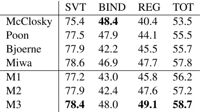
Table 1: F1 scores for the development set of Task 1 of the BioNLP 2009 shared task.

task consist of 797, 150 and 250 documents, respec-tively.

Table 1 shows our results for the development set. We compare our three models (M1, M2 and M3) and previous state-of-the-art systems: McClosky (Mc-Closky et al., 2011a), Poon (Poon and Vander-wende, 2010), Bjoerne (Björne et al., 2009) and

Miwa(Miwa et al., 2010b; Miwa et al., 2010a). Pre-sented is F1 score for all events (TOT), regulation events (REG), binding events (BIND) and simple events (SVT).

Model 1 is outperforming the previous best joint models of Poon and Vanderwende (2010), as well as the best entry of the 2009 task (Björne et al., 2009). This is achieved without careful tuning of thresh-olds that control flow of information between trigger and argument extraction. Notably, training Model 1 takes approximately 20 minutes using a single core implementation. Contrast this with 20 minutes on 32 cores reported by Poon and Vanderwende (2010).

Model 2 focuses on regulation structures and re-sults demonstrate this: F1 for regulations goes up by nearly 2 points. While the impact of joint modeling relative to weaker local baselines has been shown shown by Poon and Vanderwende (2010) and Riedel et al. (2009), our findings here provide evidence that it remains effective even when the baseline system is very competitive.

With Model 3 our focus is extended to binding events, improving F1 for such events by at least 5 F1. This also has a positive effect on regulation events, as regulations of binding events can now be more accurately extracted. In total we see a 1.1 F1 in-crease over the best results reported so far (Miwa et al., 2010b). Crucially, this is achieved using only a single parse tree per sentence, as opposed to three

SVT BIND REG TOT McClosky 68.3 46.9 33.3 48.6

Poon 69.5 42.5 37.5 50.0

Bjoerne 70.2 44.4 40.1 52.0

Miwa 72.1 50.6 45.3 56.3

M1 71.0 42.1 41.9 53.4

M2 70.5 41.3 43.6 53.7

M3 71.1 52.9 45.2 55.8

M3+enju 72.6 52.6 46.9 57.4

Table 2: F1 scores for the test set of Task 1 of the BioNLP 2009 shared task.

used by Miwa et al. (2010a).

Table 2 shows results for the test set. Here with Model 1 we again already outperform all but the re-sults of Miwa et al. (2010a). Model 2 improves F1 for regulations, while Model 3 again increases F1 for both regulations and binding events. This yields the best binding event results reported so far. No-tably, not only are we able to resolve binding am-biguity better. Binding attachments themselves also improve, as we increase attachment F1 from 61.4 to 62.7 when going from Model 2 to Model 3.

Miwa et al. (2010b) use two parsers to generate their input features. For fairer comparison we aug-ment Model 3 with syntactic features based on the

enjuparser (Miyao et al., 2009). With these features (M3+enju) we achieve the best results on this dataset reported so far, and outperform Miwa et al. (2010b) by 1.1 F1 in total, 1.6 F1 on regulation events and 2.0 F1 on binding events.

We also apply Model 3, with slight modifications, to the BioNLP 2009 task 2 which requires cellu-lar locations to be extracted as well. With 53.0 F1 we fall 2 points short of the results of Miwa et al. (2010b) but still substantially outperform any other reported results on the dataset. More parse trees may again substantially improve results, as well as task-specific constraint and feature sets.

5.4 Shared Task 2011

Genia Task 1 Infectious Diseases

System TOT System TOT

M3+Stanford 56.0 M3+Stanford 55.6

M3 55.2 M3 53.4

UTurku 53.3 Stanford 50.6

MSR-NLP 51.5 UTurku 44.2

ConcordU 50.3 PNNL 42.6

Table 3: F1 scores for the test sets of two tracks in the BioNLP 2011 Shared Task.

The top five entries are shown in table 3. Model 3 is the best-performing system that does not use model combination, only outperformed by a version of Model 3 that includes Stanford predictions (Mc-Closky et al., 2011b) as input features (Riedel et al., 2011). Not shown in the table are results for full pa-pers only. Here M3 ranks first with 53.1 F1, while M3+Stanford comes in second with 52.7 F1.

The Infectious Diseases (ID) track of the 2011 task has 152 train, 46 development and 118 test documents. Relative to Genia it provides less data and introduces more types of entities as well as the biological process event type. Incorporating these changes into our models is straightforward, and hence we omit details for brevity.

Table 3 shows the top five entries for the Infec-tious Diseases track. Again Model 3 is the best-performing system that does not use model combi-nation, outperformed only by Model 3 with Stanford predictions as features. We should point out that the feature sets and learning parameters were kept constant when moving from Genia to ID data. The strong results we observe without any tuning to the domain indicate the robustness of joint modeling.

5.5 Runtime Behavior

Table 4 shows the asymptotic complexity of our three models with respect tom = _|Trig(x)_|, n =

|Cand(x)_| and p = _|Prot(x)_|. We also show the

number of iterations needed on average, the average time in milliseconds per sentence,3_{and the fraction}

of sentences we get certificates of optimality for. As expected, Model 1 is most efficient, both asymptotically and on average. Given that its ac-curacy is already good, it can serve as a basis for

3_{Measured without preprocessing and feature extraction.}

Complexity Iter. Time Exact

M1 O(nm) 1.0 60ms 100%

M2 O(Rnm) 10.4 183ms 96%

M3 O Rnm+Rp2m 11.7 297ms 94%

Table 4: Complexity and Runtime Behavior.

large-scale extraction tasks. Models 2 and 3 re-quire several iterations and more time, while pro-viding slightly less certificates. However, given the improvement in F1 they deliver, and the fact prepro-cessing steps such as parsing would still dominate the average time, this seems like a reasonable price to pay.

6 Conclusion

We presented three joint models for biomedical event extraction. Model 1 reaches near-state-of-the-art results, outperforms all previous joint models and has quadratic runtime guarantees. By explicitly capturing regulation events (Model 2), and binding events (Model 3) we achieve the best results reported so far on several event extraction tasks. The runtime penalty we pay is kept minimal by using dual de-composition. We also show how dual decomposition can be used for constraints that go beyond coupling equalities.

We use joint models, a decomposition technique and supervised online learning. This recipe can be successful in many settings, but requires expensive manual annotation. In the future we want to inte-grate weak supervision techniques to train extractors with existing biomedical databases, such as KEGG, and only minimal amounts of annotated text.

Acknowledgements

References

Jari Björne, Juho Heimonen, Filip Ginter, Antti Airola, Tapio Pahikkala, and Tapio Salakoski. 2009. Extract-ing complex biological events with rich graph-based feature sets. InProceedings of the Natural Language Processing in Biomedicine NAACL 2009 Workshop (BioNLP ’09), pages 10–18, Morristown, NJ, USA. Association for Computational Linguistics.

Eugene Charniak and Mark Johnson. 2005. Coarse-to-fine n-best parsing and maxent discriminative rerank-ing. InProceedings of the 43rd Annual Meeting of the Association for Computational Linguistics (ACL ’05), pages 173–180.

Koby Crammer and Yoram Singer. 2003. Ultraconserva-tive online algorithms for multiclass problems. Jour-nal of Machine Learning Research, 3:951–991. Ulrich Germann, Michael Jahr, Kevin Knight, Daniel

Marcu, and Kenji Yamada. 2001. Fast decoding and optimal decoding for machine translation. In Proceed-ings of the 39th Annual Meeting of the Association for Computational Linguistics (ACL ’01), pages 228–235. Jin-Dong Kim, Tomoko Ohta, Sampo Pyysalo, Yoshi-nobu Kano, and Jun’ichi Tsujii. 2009. Overview of bionlp’09 shared task on event extraction. In

Proceedings of the Natural Language Processing in Biomedicine NAACL 2009 Workshop (BioNLP ’09). Jin-Dong Kim, Sampo Pyysalo, Tomoko Ohta, Robert

Bossy, and Jun’ichi Tsujii. 2011. Overview of BioNLP Shared Task 2011. In Proceedings of the BioNLP 2011 Workshop Companion Volume for Shared Task, Portland, Oregon, June. Association for Computational Linguistics.

Nikos Komodakis, Nikos Paragios, and Georgios Tziri-tas. 2007. Mrf optimization via dual decomposition: Message-passing revisited. InProceedings of the 11st IEEE International Conference on Computer Vision (ICCV ’07).

Terry Koo, Alexander M. Rush, Michael Collins, Tommi Jaakkola, and David Sontag. 2010. Dual decomposi-tion for parsing with nonprojective head automata. In

Proceedings of the Conference on Empirical methods in natural language processing (EMNLP ’10). David McClosky and Eugene Charniak. 2008.

Self-training for biomedical parsing. InProceedings of the 46th Annual Meeting of the Association for Computa-tional Linguistics (ACL ’08).

David McClosky, Mihai Surdeanu, and Chris Manning. 2011a. Event extraction as dependency parsing. In

Proceedings of the 49th Annual Meeting of the Associ-ation for ComputAssoci-ational Linguistics (ACL ’11), Port-land, Oregon, June.

David McClosky, Mihai Surdeanu, and Christopher D. Manning. 2011b. Event extraction as dependency parsing in bionlp 2011. InBioNLP 2011 Shared Task.

R. McDonald and F. Pereira. 2006. Online learning of approximate dependency parsing algorithms. In

Proceedings of the 11th Conference of the European Chapter of the ACL (EACL ’06), pages 81–88. Ivan Meza-Ruiz and Sebastian Riedel. 2009. Jointly

identifying predicates, arguments and senses using markov logic. In Joint Human Language Technol-ogy Conference/Annual Meeting of the North Ameri-can Chapter of the Association for Computational Lin-guistics (HLT-NAACL ’09).

Makoto Miwa, Sampo Pyysalo, Tadayoshi Hara, and Jun’ichi Tsujii. 2010a. A comparative study of syn-tactic parsers for event extraction. InProceedings of the 2010 Workshop on Biomedical Natural Language Processing, BioNLP ’10, pages 37–45, Stroudsburg, PA, USA. Association for Computational Linguistics. Makoto Miwa, Sampo Pyysalo, Tadayoshi Hara, and

Jun’ichi Tsujii. 2010b. Evaluating dependency rep-resentation for event extraction. InProceedings of the 23rd International Conference on Computational Lin-guistics, COLING ’10, pages 779–787, Stroudsburg, PA, USA. Association for Computational Linguistics. Makoto Miwa, Rune Saetre, Jin-Dong D. Kim, and

Jun’ichi Tsujii. 2010c. Event extraction with com-plex event classification using rich features.Journal of bioinformatics and computational biology, 8(1):131– 146, February.

Yusuke Miyao, Kenji Sagae, Rune Sætre, Takuya Mat-suzaki, and Jun ichi Tsujii. 2009. Evaluating contribu-tions of natural language parsers to proteprotein in-teraction extraction. Bioinformatics/computer Appli-cations in The Biosciences, 25:394–400.

Hoifung Poon and Lucy Vanderwende. 2010. Joint Infer-ence for Knowledge Extraction from Biomedical Lit-erature. InHuman Language Technologies: The 2010 Annual Conference of the North American Chapter of the Association for Computational Linguistics, pages 813–821, Los Angeles, California, June. Association for Computational Linguistics.

Vasin Punyakanok, Dan Roth, Wen tau Yih, and Dav Zi-mak. 2004. Semantic role labeling via integer linear programming inference. InProceedings of the 20th in-ternational conference on Computational Linguistics (COLING ’04), pages 1346–1352, Morristown, NJ, USA. Association for Computational Linguistics. Sebastian Riedel and James Clarke. 2006.

Incremen-tal integer linear programming for non-projective de-pendency parsing. InProceedings of the Conference on Empirical methods in natural language processing (EMNLP ’06), pages 129–137.

Natural Language Processing in Biomedicine NAACL 2011 Workshop (BioNLP ’11), June.

Sebastian Riedel, Hong-Woo Chun, Toshihisa Takagi, and Jun’ichi Tsujii. 2009. A markov logic approach to bio-molecular event extraction. InProceedings of the Natural Language Processing in Biomedicine NAACL 2009 Workshop (BioNLP ’09), pages 41–49.

Sebastian Riedel, David McClosky, Mihai Surdeanu, Christopher D. Manning, and Andrew McCallum. 2011. Model combination for event extraction in BioNLP 2011. In Proceedings of the Natural Lan-guage Processing in Biomedicine NAACL 2011 Work-shop (BioNLP ’11), June.

Sebastian Riedel. 2008. Improving the accuracy and ef-ficiency of MAP inference for markov logic. In Pro-ceedings of the 24th Annual Conference on Uncer-tainty in AI (UAI ’08), pages 468–475.

D. Roth and W. Yih. 2004. A linear programming formu-lation for global inference in natural language tasks. In

Proceedings of the 8th Conference on Computational Natural Language Learning (CoNLL’ 04), pages 1–8. Alexander M. Rush, David Sontag, Michael Collins, and

Tommi Jaakkola. 2010. On dual decomposition and linear programming relaxations for natural lan-guage processing. InProceedings of the Conference on Empirical methods in natural language processing (EMNLP ’10).