Design of A Novel Sliding Mode Observer for Chaotic Systems

Design of A Novel Sliding Mode Observer for Chaotic Systems

H.R. Sabouhi

1

, A. A. Gharaveisi

1

, S.M.R. Rafiei

2

,

S.M.A.Mohammadi

1

,

S.M. Vaezi-Nejad

3

Abstract -

This paper describes the state

reconstruction of nonlinear chaotic systems with

uncertainty having unknown bounds. The new

observer presents simple structures that contain

a sliding mode term which is established from the

available output measurements. To the best of

authors’ knowledge, in iteration such classes of

observer have not been used in synchronization

problem. The convergence of the proposed

observer has been proved by Lyapunov

inequality equation; LMI; while the performance

of the system has been verified by famous chaotic

systems such as Lorenz and Rossler . A design

procedure for the proposed technique is

described and simulation results are presented to

show that the proposed chaos observer is vary

efficient with regards to the class of chaotic

systems.

Keywords: sliding mode Observer, chaotic system, nonlinear system1.

Introduction

Chaotic synchronization has received the attention of researches in many fields since the 1980[1-5] and is still an area of active research [6-10]. Recently information theories and concepts were applied to analyze and to quantify synchronization [11–15]. Mutual information measures have been introduced in the past for evaluating the degree of chaotic synchronization[12,13]. The methods of symbolic dynamics have also been used to relate synchronization precision to capacity of the information channel and to the entropy of the drive system[11-14]. It is well known that the study of the synchronization problem for nonlinear systems has been very important for sciences, in particular the applications to biology, medicine, cryptography, secure data transmission and so on. In general, the synchronization research has been focused onto two areas.

1. Shahid Bahonr University of Kerman, Iran 2. Shahrood University of Technology, Iran

The first one relates to the employment of state observers, where the main applications lie on the synchronization of nonlinear oscillators. The second one is the use of control laws, which allows achieving the synchronization with different structure/ order among nonlinear oscillators [16]. A particular interest is the connection between the observers for nonlinear systems and chaos synchronization, which is also known as master–slave configuration. Thus, chaos synchronization problem can be regarded as observer design procedure, where the coupling noise is viewed as an output and the slave system is the observer [17]. The main approaches, which are related to the construction of asymptotic observers for nonlinear processes, use geometric differential methods. The idea is to find a state transformation to represent the system as a linear equation plus a nonlinear term, which is a function of the system output. However, finding a nonlinear transformation that places a system of order n into the so-called observer canonical form requires the integration of n coupled partial differential equations. Furthermore, this approach needs an accurate knowledge of the nonlinear dynamics of the system.

The early works dealing with sliding mode observers which consider measurement noise were proposed by Utkin and Drakunov [18]. They discussed the state estimation using sliding mode technique. Anulova [19] treated an analysis of systems with sliding mode in the presence of noises. Slotine et. al. [20], successfully designed, so named, sliding-mode approach to construct observers which are highly robust with respect to noises in the input of the system. But, it turns out that the corresponding stability analysis can not be directly applied in the situations with the output noise (or, mixed uncertainty) presence. So, it is still a challenge to suggest a workable technique to analyze the stability of identification error generated by sliding-mode (discontinuous non-linearity) type observers [20-24].

2. Problem formulation and assumption

Consider the nonlinear system and a measurement model of the form

Cx y

x f x

= = ( ),

& ₍₁₎

Where:

x

∈

ℜ

n is the state to be estimated from,

p

y

∈

ℜ

is the measured output, f(x) is bounded

unknown and C is the constant matrix. We can write Eq.( 1) in the following form:

Cx y

u x F Ax x

= +

= ( , )

& ₍₂₎

Where:

A

∈

ℜ

n×n is a linear time inverting matrix,

pair of (A,C) are observable and

F

:

ℜ

n

→

ℜ

is the

nonlinear function that may have perturbations.

2.1 Theorem 1

Supposeachaotic system having the form as Eq.(2) and for

∀

(

x

₁

,

u

₁

),

(

x

₂

,

u

₂

)

∈

ℜ

n, the function F(x,u) satisfies the Lipschitz condition on

ℜ

n, that is

) , ( ) , ( ) , ( ) ,

(x1 u1 F x2 u2 L x1 u1 x2 u2

F − ≤ − (3)

Where: L〉0 is Lipschitz constant and

.

is the

standard Euclidean norm in

ℜ

n.

We consider

) ( )

(_{x Ax P} 1_{C h x}

f _{− =} − T ₍₄₎

Where:

h

(

x

_t

,

u

_t

)

is bounded as

h

〉

h

(

x

,

u

)

3. Sliding mode observer design

For the above system, the following sliding mode observer is designed:

(5)

Where eis the state reconstruction error, defined as

x

x

e

=

−

ˆ

and ey is output error defined as ey=

y

−

y

ˆ

=C

Δ

=C (

x

−

x

ˆ

) = Ce

)

,

ˆ

(

x

e

S

is selected as

) ( )

, ˆ

( y sign ey

C C e

x

S =− Γ

Δ Δ Γ −

= ρ ρ (6)

Now we can reconstruct the observer in the following form:

x

C

y

e

sign

e

H

x

A

x

_{y y}

ˆ

ˆ

)

(

)

(

ˆ

ˆ

=

Γ

+

+

=

ρ

&

         (7)

Where the gain matrix H and the switching gain ρare chosen such that the stability of the observer system is preserved. The discontinuous feedback input is defined as:

⎪⎩ ⎪ ⎨ ⎧

〈 −

〉 +

=

0 ,

1

0 ,

1 ) (

y y

y _e

e e

sign (8)

Since the sliding mode observer is not dependent on

nonlinear plant, only the output y is needed. The

derivative of the observer error is:

e

_&

= Ae − HCe + F(x, u) −ρΓ sgn(Ce) (9) = (A − HC)e + F(x, u) −ρΓ sgn(Ce)

The feedforward gain matrix H can be obtained in

two ways; pole assignment method and LQ method. For the latter method, it is easier to derive the gain matrix H using Riccati equation as:

AP + PAT_{− PC}T_R−1_{CP = −Q (10)}

Where Q and R are arbitrary semi-positive definite and positive definite matrices, respectively. Equation (10) has a positive definite solution for P. Then AT

−CT_HT _{is stable assuming:}

HT _{= R}−1_{CP (11)}

x C y

e x S e H x A

x _y

ˆ ˆ

) , ˆ ( ) ( ˆ ˆ

=

+ +

=

Which is equivalent to the stability of َA0= A−HC. In fact, H is the observer gain matrix for the system Eq. (2).

By using appropriate Lyapunov equation, we select a

Γ

such that the reconstruction error system is

asymptotically stable. Let Pf be the positive definite solution of the Lyapunov equation as:

A0Pf + PfA0T = −Qf (12)

Where Qf is an arbitrary positive definite matrix.

Let set:

ΓT_P

f = C (13)

3.1 Theorem 2

If f is bounded, the observer gain satisfies the

following Equation:

ρ

>

h

(14)

Then the error between the sliding mode observer and the nonlinear system is asymptotically stable

means that: lim =0

∞

→ e

t .

Proof Let consider the a Lyapunov function

candidate for Eq.(9) as:

V(e) = eT_P

f e (15) Then;

V(e) = ˙eT_P

f + eTPf˙e = eT (A0Pf+ Pf A0T)e + (F −ρΓT _sign(ce))P

fe + eT_P

f (F −ρΓT sign(ce)) = −eT_Q

f e + 2(PfeF −ρΓTPf e sign(ey)) = −eT_Q

f e + 2eTPf[S(

x

ˆ

,ey) +F(x,u)]

By using (5) we have:

)

,

(

),

,

(

)

,

(

_x

_u

_P

1

_C

_h

_x

_u

_h

_x

_u

F

T

f−

=

<

ρ

If we select

S

(

x

ˆ

,

e

_y

)

and

Γ

as (6), (13); we have

V

&

= - eT_Q

fe+2eTCTh(x,u)

Δ

Δ

Γ

−

C

C

ρ

2

= - eT_Q

fe+2eTCTh(x,u)-

2

ρ

C

Δ

≤ - eT_Q

fe+2 CΔ ( h(x,u) −ρ)≤ 0 (16)

Since it is assumed that

V

&

≤ 0, e

∈

L

_∞, from the error equation (9) it is also

e

_&

∈

L

_∞ and V is

bounded process, e is quadratically inerrable and

bounded. Using Barbalat,s Lemma we obtain that

the observer error e is asymptotically stable,

then

lim

=

0

∞ →

e

t .

4. Simulation results

4.1 Example 1

In this section we consider Lorenz system, which is known to exhibit a chaotic behavior to verify the effectiveness of the proposed methods in this paper [29]. The dimensionless version of Lorenz system is:

3 2 1 3

2 1 3 1 2

1 2

1

(

)

bx

x

x

x

x

rx

x

x

x

x

x

x

−

=

−

+

−

=

−

=

&

&

&

σ

With the measurement of equation y=x1, and

choosing

σ

=10,r=28,b=8/3 then the system exhibits chaotic observer. Initial conditions are chosen as:

3

)

0

(

ˆ

,

4

)

0

(

ˆ

,

5

)

0

(

ˆ

3

)

0

(

,

4

)

0

(

,

5

)

0

(

3 2

1

2 2

1

−

=

−

=

−

=

=

=

=

x

x

x

x

x

x

In this paper we assume that Q =50eye(3)

,Qf=100eye(3),

ρ

=

0

.

2

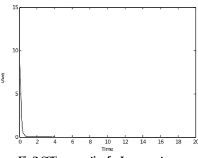
and R=1. Simulation results are given in Figures 1,2 and 3. Fig. 2 shows the state error that rapidly converges to zero. Note that we assumed that the sampling period is T = 9× 10-3 _{s and}

we defined the sum squared error (SSE) as:

2 3 3 2 2 2 2 1

1

ˆ

)

(

ˆ

)

(

ˆ

)

(

x

x

x

x

x

x

Sse

=

−

+

−

+

−

0 0.5 1 1.5 2 2.5 3 -15

-10 -5 0 5 10 15 20

Time

state1 observed 1

0 0.5 1 1.5 2 2.5 3

-15 -10 -5 0 5 10 15 20 25 30

Time

state2 observed 2

0 0.5 1 1.5 2 2.5 3

-10 0 10 20 30 40 50

Time

[image:4.595.90.255.122.497.2]

state3 observed 3

Fig .1 Drive state for Lorenz system

0 5 10 15 20

-5 0 5 10

Time Er

orr

[image:4.595.325.523.123.280.2]

e1 e2 e3

Fig.2 Synchronization state errors of Lorenz system

0 2 4 6 8 10 12 14 16 18 20

0 5 10 15

Time Ss

e

Fig.3 SSE propagation for Lorenz system

4.2 Example 2

In this example we consider Rössler system. Such a system can be implemented by a chemical reaction scheme[25-27]. It contains only one nonlinear term but produces a high-dimensional chaos phenomenon with two directions of hyper chaotic instability on the attractor. A four-variable Rössler system can be described by the following differential equations:

1

3 3

2 3

3 2 1 1

2 1

)

(

x

y

x

f

G

x

x

x

x

x

x

x

x

x

=

−

−

=

+

−

=

−

=

α

α

α

β

&

&

&

Where:

α

=

(

C

₂

/

C

₁

)

and

β

=

(

C

₂

/

LG

2

)

. The following parameters are assumed

11

,

8

,

05

.

,

8

.

0

2

1

=

−

G

=

−

α

=

β

=

G

& G=0.7[30].

With these parameters, the equations given above exhibit a double scroll type chaotic behavior.

Initial conditions are chosen as:

4

)

0

(

ˆ

,

5

)

0

(

ˆ

,

5

)

0

(

ˆ

4

)

0

(

,

5

)

0

(

,

5

)

0

(

3 2

1

2 2

1

=

=

−

=

−

=

−

=

=

x

x

x

x

x

x

0 5 10 15 20 -10

-5 0 5 10 15

Time

state2 observed 2

0 5 10 15 20

-5 0 5 10 15 20 25

Time

[image:5.595.92.268.123.394.2]

state3` observed 3

Fig.4 Drive state for Rössler system

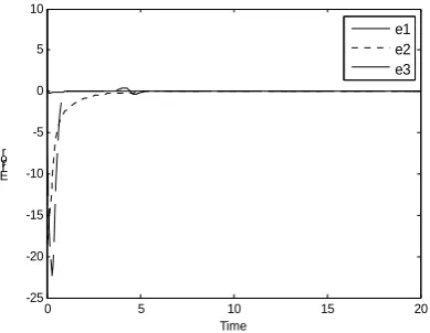
From Fig.5 it can be seen that the error of the state converges to zero.

0 5 10 15 20

-25 -20 -15 -10 -5 0 5 10

Time Err

or

e1 e2 e3

Fig.5 Synchronization state errors of Rössler system

Figure 6 shows the sum squared error (SSE).

0 5 10 15 20

0 5 10 15 20 25 30

Time Ss

e

Fig.6 SSE propagation for Rössler system

The results achieved in this paper show that

e

converges to zero more rapidly and the observer performance is very efficient.

5. Conclusions

In this paper a sliding mode observer is proposed to reconstruct the states of uncertain nonlinear systems from available output measurements. The proposed approach is robust for synchronization despite the difference between transmitter and receiver parameters and their initial conditions. We have applied this approach on three systems, Lorenz,

Rössler and Chuaיs circuit. With reference to the

simulation results, it is shown that the correct estimation of real system can be obtained. The effectiveness of the proposed method is investigated through some examples that show a significant performance improvement.

6. Acknowledgements

[image:5.595.77.272.462.613.2]

References

[1] E. Dudnik, Y. Kuznetsov, I. Minakova, and Y. Romanovskii, Vestn. Mosk. Univ., Ser. 3: Fiz., Astron. 24, 1983, p84.

[2] H. Fujisaka and T. Yamada, Prog. Theor. Phys. 69,

1983, p.32.

[3] V. Afraimovich, N. Verichev, and M. Rabinovich, Radiophys. Quantum Electron. 29, 1987, p.795

[4] L.M. Pecora and T. L. Carroll, Phys. Rev. Lett. 64,

1990, p.821

[5] Morgul O, Solak E. Observer based synchronization of chaotic systems. Phys Rev E 1996;54:4803–11. [6] A. Pikovsky, M. Rosenblum, and J. Kurths,

Synchronization: A Universal Concept in Nonlinear Sciences _Cambridge University Press, Cambridge, (2001).

[7] S. Boccaletti, J. Kurths, G. Osipov, D. Valladares, and C. Zhou, Phys. Rep. 366, 2002, p.1

[8] U. S. Freitas, E. E. N. Macau, and C. Grebogi, Phys. Rev. E 71, 2005, p.47203

[9] A. Fradkov and A. Pogromsky, Introduction to

Control of Oscillations and Chaos _World

Scientific, Singapore, 1998.

[10] L. M. Pecora and T. L. Carroll, Phys. Rev. Lett.

80, 1998, p.2109.

[11] T. Stojanovski, L. Kočarev, and R. Harris, IEEE Trans. Circuits Syst., I: Fundam. Theory Appl. 44,

1997, p.1014.

[12] M. Paluš, V. Komárek, Z. Hrnčir, and K. Štěrbová, Phys. Rev. E 63, 2001, p.46211.

[13] A. Shabunin, V. Demidov, V. Astakhov, and V. Anishchenko, Phys. Rev. E 65, 2002, p.56215.

[14] S. D. Pethel, N. J. Corron, Q. R. Underwood, and K. Myneni, Phys. Rev. Lett. 90, 2003, p.254101.

[15] M. S. Baptista and J. Kurths, Phys. Rev. E 72,

2005, p.45202(R).

[16] Wu WC, Chua LO. A unified framework for synchronization and control of dynamical systems. Int J Bifurcat Chaos 1994;p.979–98.

[17] Nijmeijer H, Mareels IM. An observer looks at synchronization. IEEE Trans Circ Syst, Part I 1997;44(10):882–90.

[18] Drakunov SV, Utkin V. Sliding mode observers. Tutorial. In: Proc 34th IEEE conference on decision and control (CDC), December 13–15, New Orleans, LA: 1995. p. 3376–8.

[19] Anulova SV. Random disturbances of the operation of control systems in the sliding mode. Automat Remote Control 1986; 47(4):474–9. Part I.

[20] Slotine J, Hedricks J, Misawa E. On sliding observers for nonlinear systems. J Dyn Meas

[21] Ushio T. Synthesis of synchronized chaotic systems based on observers. Int J Bifurcat Chaos 1999;9(3):541–6.

[22] Martinez-Guerra R, Cruz-Victoria JC, Gonzalez-Galan R, Aguilar-Lopez R. A new reduced-order observer design for the synchronization of Lorenz system. J Chaos Sol Fract 2006;28:511– 7.

[23] Walcott BL, Corles MJ, _ Zak SH. Comparative study of non-linear state-observation techniques. Int J Control 1987;45(6):2109–32.

[24] Isidori A. Nonlinear control system. 3rd ed. London: Springer-Verlag; 1995.

[25]Alexander L. Fradkov and Boris Andrievsky. Chaotic observer-based synchronization under information constraints. PHYSICAL REVIEW E

73, 2006, p.66209

[26] Il-Song Kim. The novel state of charge estimation method for lithium battery using sliding mode observer. Journal of Power Sources 163 (2006) 584–590

[27] Wen Yu, "Sliding Mode Technique and Sliding Mode Observer," 2003-06-02.