Effective granularity in Internet badhood detection: Detection rate, Precision and Implementation performance

UNIVERSITY OF TWENTE

Faculty of Electrical Engineering, Mathematics and Computer Science

Design and Analysis of Communication Systems group

MASTER OF SCIENCE THESIS

Effective granularity in Internet badhood detection:

Detection rate, Precision and Implementation

performance

by

Ali Davanian

Committee:

Prof. dr. ir. A.

Pras

A.

Warmenhoven (Redsocks Security)

Dr. A.

Sperotto

Dr. G.

Moura

Abstract

New malicious nodes appear everyday on the Internet. Previous studies have shown that these nodes are not randomly distributed on the Internet; similar to the high density of criminal activities in real world bad neighborhoods, there exist Internet bad neighborhoods. Two common features to draw the local net-work boundaries within Internet and hence identifying the bad neighborhoods are fixed /24 IP prefix and dynamic Border Gateway Protocol (BGP) IP prefix. The main difference between these two features is the size of the underlying neighborhood and hence the granularity in the measurement of malicious activ-ity. In this study, by analyzing a dataset of Command and Control servers and botnets, we show that BGP prefix is preferred in identifying bad neighborhoods because it offers 8% better detection rate in identifying new malicious nodes. In summary, our contributions in this study are:

1. We show that likelihood of having malicious activity from a neighborhood is a precise metric for malice prediction based on regression modeling

2. We show that likelihood of having malicious activity in adjacent /24 pre-fixes within a BGP prefix is very similar with a 4% of change on average and hence the loss of granularity by using BGP is negligible

3. We show that BGP prefixes offer a detection rate improvement of 8%

4. We conclude that based on precision, granularity, detection rate and lookup performance BGP is a better feature for Internet bad neighborhood iden-tification

Acknowledgments

This Master thesis marks the end of my two-year graduate program in Security and Privacy. The current work would not have been possible without the con-tribution and support of many great people. Firstly, I would like to thank my daily supervisor Adrianus Warmenhoven. Adrianus is one of the few great white hat hackers who also has a great academic acumen. I learned many things from Adrianus both scientifically and socially, and now that I am writing this part of my thesis, I feel sad that my journey with this great mentor has come to an end.

Secondly, I had the honor to be supervised by Professor Aiko Pras. I don’t know many professors like Prof. Pras; he is a highly respected man in our field but still very modest and lovely. His modesty allows one to grow, contribute and learn. I would like to express my highest level of gratitude to this great man for all he taught me. Without Prof. Pras’ supervision, my contribution in this work would not have been possible.

Thirdly, I would also like to thank Dr. Giovane Moura. Giovane is a friendly and highly insightful supervisor. As the author of Internet Bad Neighborhoods, he helped a lot to further my research. Giovane patiently spent hours with me discussing my research direction. His efforts and sharp comments increased the value of the current work.

I would like to thank Dr. Ana Sperotto and Dr. Rick Hofstede for their invaluable efforts in the beginning of this research. Without their efforts, the current work would not have been possible. Rick not only helped me to for-mulate my research questions but also introduced me to many great people. Although he had to inevitably terminate his supervision, I always appreciate his influence in my academic works.

Contents

1 Introduction 9

1.1 Background . . . 12

1.2 Granularity . . . 13

1.2.1 Example. . . 14

1.3 Research Questions . . . 15

1.3.1 Approach . . . 16

1.4 Research Value . . . 17

1.5 Summary . . . 17

2 Literature Review 19 2.1 Reputation Oracle . . . 20

2.2 Reputation Function . . . 21

2.3 Reputation output . . . 22

2.4 Aggregation feature . . . 23

2.5 Benchmarking. . . 24

2.6 Summary . . . 25

3 Problem Formulation and Definitions 27 3.1 Likelihood . . . 28

3.2 Basic definitions . . . 29

3.2.1 Example. . . 30

3.3 Metrics definition . . . 30

3.3.1 Granularity Delta . . . 30

3.3.2 Detection Rate . . . 31

3.3.3 Lookup performance . . . 32

3.3.4 Precision . . . 33

3.4 Summary . . . 33

4 Aggregated Reputation Lookup Implementation 35 4.1 Indexing Search Algorithm (ISA) . . . 36

4.1.1 Data Structure . . . 36

4.1.2 Initialization . . . 36

4.1.3 Searching . . . 38

8 CONTENTS

4.2.1 Data structure . . . 39

4.2.2 Initialization . . . 39

4.2.3 Searching . . . 39

4.3 Summary . . . 40

5 Data Collection Methodology 41 5.1 Redsocks Raw Dataset . . . 41

5.1.1 Indicators Of Compromise. . . 42

5.1.2 IOC Sources . . . 42

5.1.3 How accurate is our raw data? . . . 42

5.2 Prefix Dataset Structure . . . 43

5.3 Preprocessing . . . 43

5.4 Generated Prefix Datasets . . . 45

6 Experimental Results 47 6.1 BGP Prefix Length Distribution . . . 47

6.2 Precision. . . 48

6.3 Granularity . . . 50

6.4 Detection Rate . . . 52

6.5 False Positive (FP) and False Negative (FN). . . 52

6.6 Lookup performance . . . 54

6.7 Summary . . . 55

7 Conclusion 57 7.1 Relation to State of The Art . . . 58

7.2 Future Work . . . 59

Chapter 1

Introduction

Internet has become an inseparable part of our daily lives. At the same time, the security of Internet world has become one of the main concerns in the world. Only in 2016, over 100000 cyber incidents were reported targeting Health institutions, financial organizations, Industrial systems etc [1]. One of the main sources of these cyber incidents is malware. Malware is a piece of program that its purpose is to do some harm to the host system it infects. For instance, one of the malware that caused much damage in 2016 was Mirai botnet [2]. This malware could temporarily paralyze part of the Internet connectivity using a type of attack known as Distributed Denial Of Service(DDOS) attack. In this type of attack, many infected hosts at the same time send traffic to a destination and hence disrupt the service. Another instance of malware that caused a cyber incident in 2017 is Wannacry ransomware. Ransomware make the data on the infected computer inaccessible to the user and ask for a ransom in return of the data. It is estimated that this malware caused $4 billion of damage [3].

Internet is actually a collection of smaller local networks that are connected together. Evidence shows that cyber attackers are more concentrated in some of these local networks than others. In order to better understand the concept, we make an analogy to the real world so called ”bad neighborhoods”. In New York, law enforcement tags some neighborhoods as ”bad” based on the number of crime reports. The crime rate in some neighborhoods is higher due to variety of reasons such as poor economy of the neighborhood. These neighborhoods in future are expected to foster more malicious activities, and henceforth, law enforcement would carefully monitor these neighborhoods. Similar to the real world, there exist bad neighborhoods in the Internet world.

Internet bad neighborhood concept can be used to predict attackers’ source addresses and mitigate cyber threats [16]. For example, figures 1.1 shows the distribution of the infected hosts by Mirai. We can see from the figure that infected hosts are more concentrated in some regions. This is because these regions, or hereafter Internet bad neighborhoods, have poor security measures in place and infection spreads quickly within them. Given this, we can prevent DDOS attack from these infected hosts by blocking traffic from them; after

10 CHAPTER 1. INTRODUCTION

Figure 1.1: Mirai distribution of infected hosts

ing malicious traffic from a few IP addresses, we can predict the attack from the remaining IP addresses of the neighborhood and hence prevent it. Identi-fying Internet bad neighborhoods enables Intrusion Detection Systems to predict attacks from neighbor nodes within a network.

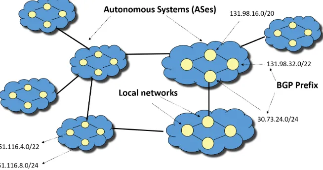
In order to identify Internet bad neighborhoods with homogeneous behavior, we need to understand the structure of Internet. Internet is composed of several

Autonomous Systems (AS), see Figure1.2. An Autonomous System is a large

network that is responsible for the distribution of traffic within the network. An AS, itself, consists of several smaller networks. The communication between different Autonomous Systems is through Border Gateway Protocol (BGP). Via Border Gateway Protocol, an AS announces the IP addresses of the smaller networks it controls i.e. through BGP prefix announcements. A BGP prefix is in X.Y.Z.W/N format where X,Y,Z and W are integers between 0 to 255 and N is an integer between 8 to 24. Based on this mechanism, the neighbor ASes pass the traffic to one another until it reaches the AS that contains the destination IP address.

Based on the above explanation, one may assume that an autonomous system is a neighborhood. Although that assumption is not wrong, the neighborhood in such case is too large. We can not expect a homogeneous malicious or benign behavior from such large entity because an AS is further split into smaller net-works that are managed by different administration entities. For instance, many of the autonomous systems are actually Internet Service Providers (ISPs). An ISP would use a BGP prefix for DSL users, a prefix for WAN users, a prefix for servers in a rack and another for a large organization such as a university. Since these prefixes are used for different purposes and have different administration entities, we can not expect the same behavior from all of them.

Two common approaches to identify an Internet neighborhood to which

an IP address belongs are based on BGP announcements and Classless

Inter-Domain Routing(CIDR) /24 prefixes, hereafter as fixed /24 prefixes. The

11

Figure 1.2: Internet Structure and Autonomous Systems

can expect same behavior from the nodes within /BGP prefixes since they have the same administration policies and are probably physically neighbors [17]. The latter is based on the logic that a BGP prefix length can be as long as 24 [13]. Hence, a /24 prefix is a smaller neighborhood within a BGP prefix.

Our research goal in this paper is to compare the Internet bad neighbor-hoods based on the BGP and fixed /24 prefixes. The difference in thesizeof the

neighborhoods derived from each approach affects the error and the latency

in the prediction of attack from an IP address. The error can be misidentifying a traffic as malicious i.e False Positive (FP) or benign i.e False Negative (FN). The low rate of FP and FN are of high importance for an Intrusion Detection System. A high FP rate results in large number of intrusion alerts that are in fact wrong. Therefore, the human operator has to manually validate the accuracy of many alerts. A high FN means many attacks remain undetected.

Size of neighborhoods has a direct impact on bothFP and FN. The larger a neighborhood, the lower false negative rate of Intrusion Detection. This is because we blacklist more IP addresses by enlarging neighborhoods. For in-stance, assume that we blacklist the entire Internet i.e the whole IP space. In this case, the FN rate is zero since we label traffic from any given IP address as malicious. On the other hand, by enlarging the neighborhood size we also increase FP rate. This is because FN and FP have reverse correlation [14]. For instance, in blacklisting the entire Internet, many of our detections are actually false because not every traffic is malicious.

12 CHAPTER 1. INTRODUCTION

1 million IP addresses. In such case, the Intrusion Detection System has to analyze the traffic from these 1 million sources and this delays the detection.

In summary, our research goal is to compare the Intrusion detection and prediction error and latency of Internet bad neighborhoods based on BGP and fixed /24 prefixes. In the following section 1.1, we discuss the background of the Internet bad neighborhood topic. In section1.2, we discuss the granularity (effect of size) of Internet bad neighborhood. In section1.3, we present our pre-cise research questions and our approach to answer those questions. In section

1.3.1, we explain the value of our research for Intrusion Detection systems.

1.1

Background

The concept of Internet bad neighborhood is built upon IP addresses reputation. IP addresses reputation is often one of the elements in a vector of features used for malice detection. Reputation of an IP address is defined based on its historical malicious activities. The reputation of an IP address is usually shown with 1 and 0 representing, in order, listing or not listing in a blacklist. The intuition behind IP address reputation is that if an attacker attacks once, it will attack again in near future and we can identify the same attacker by its IP address. For instance, IP reputation, among other features, is used in [4,5] for spam detection. In [6], IP reputation is used in a vector of features to detect malicious DNS addresses. Since reputation by definition depends on the historical records, it has limited capability in malice detection; we must have already detected malicious activity for an IP address in order to further blacklist it.

Single IP address reputation has several limitations. Firstly, IP addresses are often leased for a short period. Due to the short leasing time [7, 8], the historical malicious activity of the current IP address can not always accurately be attributed to the endpoint (source or destination of a traffic) that holds the IP address. Secondly, the IP address space is 4G large. Tracking the reputation of all these nodes is expensive in a sense that we need to have traffic data from all the 4G space in order to detect all the malicious addresses. We also need to store the reputation of these nodes that might be expensive for network appliances with limited disk space and memory size. As a result, False Negative (FN) rate of IP blacklists is high [9]. Sinha et al measure the effectiveness of blacklists for Spam Detection. They find out that 21% of the traffic that Spam detectors such as SpamAssassin can detect remain undetected by blacklists. This is mainly because a large portion of the missed sources (around 90%) are observed for just one second in the network [9]. Such a short lifetime would not allow blacklist maintainers to effectively identify and report such malicious sources.

1.2. GRANULARITY 13

their result, it’s likely to see more malicious activity from the same network of an already seen malicious host, similar to dangerous neighborhoods in the real world. [11,12, 4, 5,13] also reach the same findings. For instance, based on the reputation of 1.1.1.1, 1.1.1.2 and 1.1.1.3 IP addresses we can derive the reputation of 1.1.1.0/30 subnet and assume that every traffic from this subnet is malicious. Several studies confirm the effectiveness of the aggregated reputation in spam detection [10,4,5,14].

1.2

Granularity

We identify Internet bad neighborhoods by aggregating the reputation of a few nodes and then attributing it to the network from where those nodes come. The aggregation of nodes reputation can be carried out with different levels of granularity and based on a feature, hereafter as aggregation feature. From a very high level view, with a low granularity, we can aggregate the reputation of the nodes within an Autonomous System (AS) and use Autonomous System Number (ASN) as the aggregation feature. Although ASN for reputation aggre-gation is used in [12,15,16] in order to find malicious Autonomous Systems, we don’t find ASN granular enough for a reputation attribution. In the following paragraphs we explain why.

Nodes within an AS are further grouped under some IP routing prefixes that may be controlled by one or more network operators. For instance, Internet Service providers may use one IP prefix for their DSL users and another for the mobile users. They may further lease an entire prefix to an organization like a university. The autonomous system identified by ASN 1103 or name SURFnet is a service provider in Netherlands that serve multiple universities and organizations under different IP prefixes. Each of these organizations has different network administration policies and hence different levels of security. Furthermore, the nodes within an organization are likely to be geographically close to each other. Henceforth, BGP prefixes are used to cluster Internet nodes in different networks [17,11,12,4, 14].

Krishnamurthy and Wang coined the term network aware clustering [17]. Via traceroute and reverse DNS resolving, they find out that 90% of IP addresses can be correctly clustered in this way. Jung et al used network aware clustering to predict IP addresses that perform DOS attack in the near future. Network aware clustering has been frequently used for spam filtering [11]. [4,14]. These works assume that BGP prefixes draw the network boundaries under the same administration. Therefore, we can assume that nodes within an administration network would expose the same behavior i.e. the IP BGP prefix would entail the neighborhood to which a node belongs. That said, the networks derived from BGP prefixes have different sizes and hence the attributed reputations have different granularities.

14 CHAPTER 1. INTRODUCTION

identify bad neighborhoods in [10,18,13]. While ASNs and BGP prefixes carry semantics and entail network boundaries, /24 prefixes are not correspondent to any specific semantics in Internet routing except that they are the smallest chunks within an ASN or BGP prefix. That said, it is unclear that fine gran-ularity of/24 aggregation leads to any particular advantage in terms of malice detection error and latency.

Since /24 prefixes are subset of a BGP prefix, the definition of neighborhood can apply to both aggregations i.e. based on BGP prefix feature or /24 prefix feature. The difference is the granularity; BGP neighborhood is a larger or same size neighborhood in comparison to /24 prefix. The level of granularity has an effect on the false positive and false negative [14]. The larger our aggregation group, the better our detection rate and false negative. At the same time, by enlarging the aggregation size and generalizing the reputation we should expect a higher false positive rate [14]. Furthermore, the difference in granularity results in the difference in the number of stored entries in our reputation database. Such difference, in turn, affects the lookup performance when inquiring the reputation database.

1.2.1

Example

The difference in the level of granularity leads to a difference in the number of black listed IP addresses. For instance, let’s analyze the AS AS31549. This ASN number belongs to Aria Shatel Company Ltd. Aria Shatel Company is an Internet Service Provider in Iran. Under this AS number, there are 230

IP V4 BGP prefixes announcement of different lengths. In total, 1,214,464

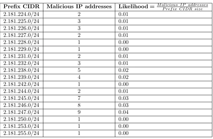
IP addresses are originated from this Autonomous system. According to our dataset, around fifty /24 prefixes that have a least one malicious IP address belong to this AS number. Seventeen of these /24 prefixes fall under one BGP

prefix announcement (see Table 1.1). Dividing the number of malicious IP

addresses within a prefix by the size of the prefix (which is 256) we get likelihoods of malicious activity between 0 and 0.04 with a median and mean of 0.01 for these seventeen prefixes. If we aggregate the reputation of these seventeen /24 prefixes by their advertised BGP prefix, which is 2.181.224.0/19, the resulted malicious activity likelihood of this BGP prefix after aggregation is 0.01.

By keeping the reputation of this BGP prefix not only we can flag a potential malicious traffic from the seventeen /24 prefixes from which we already observed malicious IP addresses but also we expand our prediction to the adjacent prefixes of these 17 prefixes. All these 32 prefixes with a malicious activity likelihood of 0.01 are represented in routing snapshots with one single BGP entry and one

organization description name ”Information Technology Company (ITC)”. Our

1.3. RESEARCH QUESTIONS 15

Prefix CIDR Malicious IP addresses Likelihood = M alicious IP addresses_{P ref ix CIDR size}

2.181.224.0/24 2 0.01

2.181.225.0/24 3 0.01

2.181.226.0/24 3 0.01

2.181.227.0/24 2 0.01

2.181.228.0/24 1 0.00

2.181.229.0/24 1 0.00

2.181.231.0/24 2 0.01

2.181.232.0/24 3 0.01

2.181.238.0/24 5 0.02

2.181.239.0/24 4 0.02

2.181.242.0/24 1 0.00

2.181.244.0/24 2 0.01

2.181.245.0/24 7 0.03

2.181.246.0/24 8 0.03

2.181.247.0/24 9 0.04

2.181.250.0/24 1 0.00

2.181.253.0/24 1 0.00

2.181.255.0/24 1 0.00

Table 1.1: /24 prefixes with malicious activity from AS31549

the AS would be_1214464106 which is epsilon. In other words, we would be penalizing 1214464 IP addresses for a malicious activity of only 106 IP addresses that mostly come from one BGP prefix. In conclusion, the underlying reason that the ASN is not granular enough is that although the AS31549 represents one ISP name, we observe around 20 different organization names that use the 256 announced prefixes. In summary, we can not expect a homogeneous behavior from a large entity such as AS but our hypothesis is that we can expect the same behavior from /24 prefixes represented by a single BGP entry.

1.3

Research Questions

As already stated in the beginning of this chapter, our main research question is:

Which of prefix types, BGP or fixed /24, is more effective in Internet bad neighborhood identification, in terms of Intrusion detection prediction error and latency?

As noted in the previous section, there are two lines of work; one line of works use BGP prefix for aggregation while the other use /24. BGP offers better false negative rate while /24 offers better false positive rate (see chapter

3 for mathematical proof). Furthermore, there will be fewer BGP entries in

comparison to /24 that may impact the latency. However, the interplay of

16 CHAPTER 1. INTRODUCTION

effect of finer granularity of fixed /24 prefix in comparison to BGP on the above parameters. Qian et al compare the granularity of BGP aggregation with that of DNS based clustering. Moura et al compare the different prefix sizes but not BGP with fixed prefixes [16].

The state of the art mainly focused on spam filtering (see chapter2) whereas we need to apply bad neighborhood for malware traffic detection. Based on the application of Internet bad neighborhood in our research, an ideal comparison would be based on false positive and false negative measurement. That said, measuring these metrics require access to network traffic and a reliable ground truth. Unfortunately, computer security domain has a tangible lack of ground truth [19]. In addition, due to privacy concerns, the author of this research could not collect any network traffic regardless of tiring efforts to address the privacy concerns of the officials.

Since measuring FP/FN is not feasible for the author, he investigates other aspects of BGP and /24 prefix aggregation that facilitate answering the main research question. The research questions that we follow in the rest of this work are:

1. How different is the granularity of BGP aggregation in comparison to /24 fixed aggregation?

2. How much is the difference in the detection rate of BGP in comparison to /24 fixed aggregation?

3. How much is the difference in the lookup performance of BGP in compar-ison to /24 fixed aggregation?

4. Which aggregation feature can more precisely predict the malice of a net-work?

5. Which aggregation can better identify bad neighborhoods based on the an-swers to the above questions?

The granularity, detection rate and precision aim to measure the detection error and the lookup performance aims to measure the detection latency of an aggregation feature in Intrusion detection and prevention. In chapter 3, we precisely define granularity, detection rate, lookup performance and precision. For now, granularity measures the malice of a Internet neighborhood based on its size. Detection rate measures the number of malicious IP addresses that we detect. Precision measures the malice prediction capability of an aggrega-tion feature. Lookup performance measures the processing time required for searching the reputation of an IP address.

1.3.1

Approach

1.4. RESEARCH VALUE 17

truth, our approach would be splitting the dataset to two training and testing sets based on different time periods. Although the ground truth problem can be addressed in this way, the lack of traffic still prevents measuring false negative and false positive rates. Due to the lack of network traffic and novelty of the application of badhood in our work, we have to define new metrics to further this research.

We first formally define aggregation and reputation and present a formal framework of metrics that allow the comparison in the context of our work. We formally define malice likelihood, granularity, precision, detection rate and lookup performance metrics (see Chapter3) that can be practically used (based on the available data) for experimental analysis. We then collect the indicators of compromise from a Malware Detection Company database. Afterwards, we extract the IP addresses and build the Internet neighborhoods based on /24 prefix feature and BGP. By using the defined metrics and the provided data, the author measures reputation in form of malice likelihood, and compare the granularity, precision, detection performance and lookup performance of the badhoods reputation extracted from one month of data. Finally, we conclude which aggregation can better identify the bad neighborhoods for malware traffic detection based on the quantitative results.

1.4

Research Value

The findings in this research will improve the prediction capability of Intrusion Detection systems as explained in section 1.2. The findings answer whether BGP or fixed /24 prefix better identifies Internet bad neighborhoods. Intrusion Detection Systems hopefully can use our results to:

1. Improve the FN, FP rate of their products without much performance compromise.

2. Automate the process of generating aggregated blacklists

As a matter of fact, the author of this research conducted this research while doing Internship in the vendor company Redsocks1_{. Such collaboration helped} the author to better identify the requirements of the vendors and the end users and consider them while comparing BGP with fixed /24 prefix.

1.5

Summary

In this chapter, we explained the motivation of our research topic and the re-search questions we will answer through the rest of this thesis. Furthermore, we explained how we aim to answer these research questions. In the rest of this thesis, in the chapter2, we first review the related works and present the find-ings of the research topic assignment that has led to the research questions of

18 CHAPTER 1. INTRODUCTION

Chapter 2

Literature Review

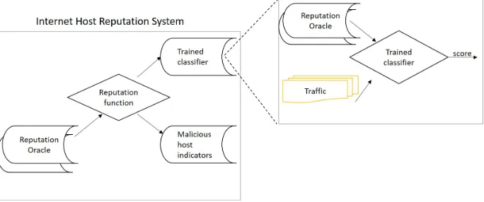
In this chapter, we review the state of the art literature that somehow uses rep-utation, hereafter as Internet Host Reputation Systems(IHRSs), for malicious detection. Internet host reputation systems output the reputation of a host based on its historical activities. The historical malicious activities, in practice, are mainly found in public blacklists based on IP or DNS address. We use the term reputation oracle for any medium that the state of the art refers to for the malicious activities of connected nodes to the Internet, hereafter as Internet hosts, in past. The data from the reputation oracle is the input to a reputa-tion funcreputa-tion in IHRSs. Different works use different reputation functions and algorithms for further processing. Eventually, the reputation output of a repu-tation system can be a trained classifier or a repurepu-tation database. The former is usually an engine that takes traffic and outputs malice based on a backend reputation oracle. The latter outputs the identifiers of malicious hosts. Differ-ent works use differDiffer-ent idDiffer-entifier metrics, hereafter as aggregation feature such as IP or DNS to identify hosts. State of the art reputation systems choose var-ious benchmarks to evaluate their results. Figure2.1shows how Internet Host Reputation Systems work in practice. This figure aims to visualize the Internet Host Reputation System’s structure and the relevance of our terminology, i.e the characteristics we use to categorize the state of the art, to these systems.

The works that we choose to review in this study are selected in a systematic way. First, we searched in google scholar based on Reputation system, Predic-tive blacklisting, Network clustering, ProacPredic-tive spam detection, Internet bad neighborhood and Internet host aggregation keywords. We removed the results older than 10 years unless the work has been a break through. Next, we selected the works that have been cited more than 10 times. Afterwards, we shortly read the papers and selected the most relevant works to our research. In the rest of this section, we compare the literature based on reputation oracle, reputation function,reputation output,aggregation feature, andBenchmarking.

20 CHAPTER 2. LITERATURE REVIEW

Figure 2.1: Internet host reputation systems

2.1

Reputation Oracle

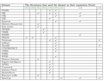
In Internet host reputation systems, the reputation is measured based on previ-ous activities of hosts. We use the term reputation oracle to refer to a database that stores the reputation of Internet hosts based on their malicious activi-ties in past. A majority of the literature use public blacklist datasets such as SURBL[20], SBL [21], CBL [22], XBL [23], Spamcop [24], Malware Domain List [25], DNS-BH [26], Zeus tracker [27], JWSDB [28], URIBL [29], SORBS [30], DSheild [31], Phishtank [32], hpHosts [33], OpenBL [34], VERIS [35], WHID [36], WPBL [37], Support Intelligence [38], UCEPROTECT[39], APWG [40], Viruswatch [41], Malware Patrol [42] and Bot Command and Control IP ad-dresses from ShadowServer Foundation [43]. A few works use Malware gener-ated traffic in a controlled environment or the traffic to a Honeypot [6][18] or Spamtrap [4][14][13] as their reputation oracle. These works record the Internet host identifier (IP, DNS name or URL) that the malicious program tries to con-nect to. Finally, a few works use the reputation computed by another product, such as IDS, to track the reputation of a host [44].

The nature of the datasets and how data is collected is different. Several datasets are providing the IP and DNS of spammers: SBL [21], CBL [22], [24], JWSDB [28] and SORBS [30]. Some other datasets identify phishing websits: SURBL[20], Phishtank [32] and APWG [40]. Datasets such as Zeus tracker [27] and Bot Command and Control IP addresses from ShadowServer Foundation [43] identify Botnet’s command and control servers. DSheild [31] provides the attackers’ addresses based on firewall and IDS logs.

2.2. REPUTATION FUNCTION 21

Dataset The literatures that used the dataset as their reputation Oracle

1 _{[45] [46] [6] [47] [15] [48] [4] [14] [13]} SURBL

SBL CBL XBL Spamcop

Malware Domain List Zeus tracker JWSDB URIBL SORBS DSheild Phishtank hpHosts OpenBL UCEPROTECT VERIS WHID WPBL Malware Domains Support Intelligence APWG Viruswatch Malware Patrol ShadowServer Honeypot traffic Spamtrap

Table 2.1: Datasets used by literature

works use. We note that few studies use the same datasets.

2.2

Reputation Function

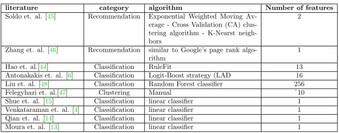
Reputation function computes the reputation of an Internet host based on some historical features of the sender. Many of the state of the art works use classifiers in order to compute the reputation based on a set of features. [5] [14] [4] [13] are simple linear classifiers that label malice based on a malicious activity threshold. The threshold is usually based on a number of historical malicious activities e.g. the number of sent spams, the number of blacklists that list an IP address or DNS, the number of IP addresses in a network that are blacklisted, or spam ratio i.e. the percentage of spams to total sent emails. Several works use sophisticated Machine Leaning (ML) classifiers and label maliciousness based on an extensive set of features [44][6][48]. [44] uses RuleFit classifier and uses 13 network and traffic related features such as message length and time of the day for classification. [6] uses Logit-Boost strategy (LAD) decision tree based on 16 domain related statistical features. These features span from number of related IP addresses and domains to the number of related malicious domains

1_{The authors of the works, in order, are Soldo et al, Zhang et al, Antonakakis et al,}

22 CHAPTER 2. LITERATURE REVIEW

literature category algorithm Number of features

Soldo et. al. [45] Recommendation Exponential Weighted Moving Av-erage - Cross Validation (CA) clus-tering algorithm - K-Nearst neigh-bors

2

Zhang et. al. [46] Recommendation similar to Google’s page rank algo-rithm

1

Hao et. al.[44] Classification RuleFit 13 Antonakakis et. al. [6] Classification Logit-Boost strategy (LAD 16 Liu et. al. [48] Classification Random Forest classifier 256 Felegyhazi et. al.[47] Clustering Manual ˜10 Shue et. al. [15] Classification linear classifier 1 Venkataraman et. al. [4] Classification linear classifier 1 Qian et. al. [14] Classification linear classifier 1 Moura et. al. [13] Classification linear classifier 1

Table 2.2: Reputation function characterization of state of the art

and lexical features of the domain name. [48] uses Random Forest classifier and a list of 258 features that are mainly related to mismanagement issues such as open resolver in the network or mis-configured HTTPS certificate.

Other works use recommendation ML algorithms to output the reputation of an Internet host [46][45]. These systems aim to build a customized blacklist for a victim. Their input is a matrix that shows which attackers attacked which

victims. They aim to find the most relevant attackers to a victim. While

[46] only searches a two-dimensional matrix to find the relevance of different attackers to a victim, [45] also takes into account the temporal behavior of the attacks and searches in a 3-dimensional space. Table2.2reports the reputation function category, the algorithm and the number of features that different works use.

2.3

Reputation output

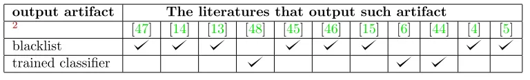
Internet Host Reputation Systems (IHRSs) usually output either of two general artifacts: blacklist; or a trained classifier. Regardless, the state of the art may use the blacklist or the classifier in a detection engine later on. For instance, [4, 14] deploy the result of reputation system they develop in SpamAssassin. Many public IHRS and state of the art works output a blacklist. Other IHRSs based on reputation usually output a trained classifier that may be used in a malicious detection engine. Detection engines that solely use blacklists usually have a less detection latency in comparison to the trained classifiers that work with multiple features because the processing would be limited to only querying the reputation of the node from the blacklist. On the other hand, the trained classifier output of an IHRS usually has a better detection performance accuracy; similar to solving a crime case by law enforcement, more evidences facilitate a better decision. In summary, detection engines based on blacklist artifact have lower detection performance accuracy while maintaining shorter detection latency in comparison to trained classifiers.

2.4. AGGREGATION FEATURE 23

output artifact The literatures that output such artifact

2 _{[47] [14] [13] [48] [45] [46] [15] [6] [44] [4] [5]}

blacklist

trained classifier

Table 2.3: Internet host reputation systems taxonomy based on output artifact

whereas a classifier is trained based on many attributes, including the Internet host address. In addition, a compiled blacklist is independent of the final im-plementation and it can be used in numerous systems e.g. firewall, IDS etc; however, a trained classifier can hardly be used anywhere else except in the designed detection engine.

A majority of state of the art output a reputation blacklist [47, 14,13, 45,

46, 15,4,5]. [6,44, 48] train a classifier based on a reputation oracle. [6] and [44] use the trained classifier in a detection engine while [48] uses the classifier to predict future cyber incidents. In addition to the previous works, there are few researches that can not be strictly characterized in one category. Table2.3

reports the characterization of the literature based on the decision time.

2.4

Aggregation feature

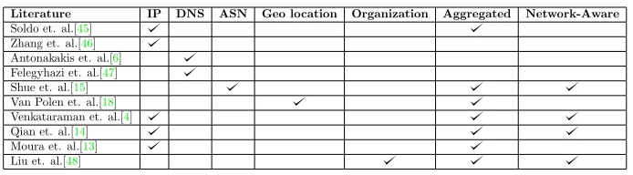
Reputation is assigned to an Internet host based on a metric by which the host can be distinguished from the others. We use the general term aggregation fea-ture to such host identifier even when there is no aggregation in practice. In such case, we consider aggregation size equal to one. Reputation is commonly as-signed to Internet hosts based onIP address[13] [45][46][4][14]. Except [46], the rest use an aggregation of IP addresses based on IP prefix. One popular alter-native to IP address isDNS address. There is usually a mapping between DNS host name and IP address through A record and vice versa through DNS PTR record. Since IP addresses are often dynamically assigned, DNS name some-times maintains more stability. [6] and [47] use DNS records. [14] uses reverse Domain authoritative reverse DNS server (rANS) and reverse DNS(rDNS) as

aggregation feature. In addition to DNS, Autonomous System Number (ASN)

can be used as an aggregation feature. The mapping between IP address and ASN is not usually intuitive; the routing BGP broadcasts need to be examined for the mapping. [15] and [49] use ASN number as aggregation feature. Finally, some works use Geo location of an Internet host such as country or city to assign reputation [50, 18].

Aggregation metric may represent an individual host or a group. IP address, and DNS A records represent an individual host while the rest of the indicators represent a group of hosts and the assigned reputation applies to all the group’s

2_{The authors of the works, in order, are Soldo et al, Felegyhazi et al, Qian et al, Moura et}

24 CHAPTER 2. LITERATURE REVIEW

Literature IP DNS ASN Geo location Organization Aggregated Network-Aware

Soldo et. al.[45] Zhang et. al.[46] Antonakakis et. al.[6] Felegyhazi et. al.[47] Shue et. al.[15] Van Polen et. al.[18] Venkataraman et. al.[4] Qian et. al.[14] Moura et. al.[13] Liu et. al.[48]

Table 2.4: IHRSs taxonomy based on aggregation feature

members. Aggregating the Internet nodes based on a metric may be carried out in different ways. For instance, IP prefix is a common method to aggregate

Internet nodes. That said, the IP prefix based on an IP addresses can be

calculated either statically and based on a fixed prefix or dynamically and based on BGP prefix. The latter is called a network aware cluster because it represents a network in real world. Several studies suggest that network aware clusters have a fine granularity, and hence the precision derived from these clusters is acceptable [4,14,51]. On the other hand, granularity increases the entries’ size that need to be stored, and hence the detection latency may increase.

Table2.4reports the result of categorizing the state of the art based on their aggregation feature. We note that systems which output a trained classifier are not mentioned in the table. The reason is that these works, as already mentioned, are taking a holistic approach; they don’t use only one metric to track the reputation. For instance, [6] uses both the IP address prefix and the Domain name of a host for training the classifier.

2.5

Benchmarking

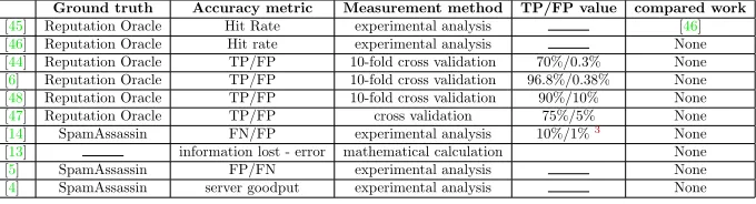
2.6. SUMMARY 25

Ground truth Accuracy metric Measurement method TP/FP value compared work

[45] Reputation Oracle Hit Rate experimental analysis [46] [46] Reputation Oracle Hit rate experimental analysis None [44] Reputation Oracle TP/FP 10-fold cross validation 70%/0.3% None [6] Reputation Oracle TP/FP 10-fold cross validation 96.8%/0.38% None [48] Reputation Oracle TP/FP 10-fold cross validation 90%/10% None [47] Reputation Oracle TP/FP cross validation 75%/5% None [14] SpamAssassin FN/FP experimental analysis 10%/1%3 _None

[13] information lost - error mathematical calculation None [5] SpamAssassin FP/FN experimental analysis None [4] SpamAssassin server goodput experimental analysis None

Table 2.5: Benchmarking of the state of the art

aggregation method improves the false positive rate of SpamAssassin by 50%. Venkataraman et. al. report the percentage of the Spams that were detected when the server was overloaded. Such measurements are not comprehensive enough to compare the malicious detection performance of their underlying reputation systems. The third category, Recommendation-based solutions, do not report based on FP and NP; they concentrate on hit count [45][46]. Hit count is calculated based on the number of blacklist entries that are seen in the actual traffic. The reason to choose this measurement is the goal of such works i.e. optimizing the size and effectiveness of the public blacklists. Table

6.1reports the characterization of the literature based on their benchmarking.

2.6

Summary

State of the art’s findings show intrusion detection based on reputation of In-ternet hosts is effective. Statistical analysis of attackers’ IP addresses show that attacks are likely to happen from the same malicious networks. Hence, clustering Internet hosts based on an aggregation features leads to detecting more attacks i.e. reducing False Negative rate and reducing the size of black-list. That said, aggregation increases False Positive(FP) while reducing False Negative(FN) based on the level of granularity.

Various aggregation features have different levels of granularity i.e. different members and group sizes. IP prefix aggregation can be based on either a fixed size or announced IP BGP prefixes, and these two have different granularities. The difference in granularity results in different detection performance (in terms of FN/FP) and detection latency. Although we can hypothesize about either detection performance or detection latency advantage of one aggregation feature solely, we can not speculate about the tradeoff of these two metrics and to extent which that granularity affects these metrics.

State of the art lack a comprehensive comparison of the different aggregation features in intrusion detection in terms of detection performance and latency. According to Tab.6.1, few works use standard accuracy metrics in their work. 3_{The reported accuracy in this work differs based on threshold and the aggregation feature.}

26 CHAPTER 2. LITERATURE REVIEW

Moreover, each work reports the measurement for one specific aggregation fea-ture; an exception is [14] that investigates the difference in granularity of IP BGP prefix aggregation vs. DNS in Spam detection. Furthermore, the state of art rarely considers also the detection latency effect of an aggregation feature. Finally, the benchmarking in various works is different, making it harder for comparing one to another.

Chapter 3

Problem Formulation and

Definitions

In the previous chapters, we explained that generalizing the reputation of the IP addresses within an BGP prefix is a common approach. Such generaliza-tion is based on the way that BGP prefixes are managed; it is expected that nodes within a BGP prefix are managed similarly, and they together form a uniform behavior. That said, BGP prefixes have different lengths and hence the granularity of the assigned reputation will be different. Decrease in the level of granularity, attributing reputation to a larger number of nodes, will affect false positive, false negative and the implementation (or processing) per-formance of the reputation aggregation. The finest granularity of a BGP prefix is for the longest length that is 24. Henceforth, aggregation based on fixed 24 length to achieve high granularity is an alternative to BGP aggregation. Yet, the advantage in doing so, in terms of measurable detection and implementation performance metrics is unclear.

The objective of this chapter is to define some formal metrics that allow the comparison of BGP and /24 fixed prefix aggregation. In chapter 1, we explain that Redsocks Security, and possibly other similar vendors, is concerned about False Positive (FP), False Negative(FN) and Performance Penalty effect of a chosen aggregation feature. However, measuring FP and FN of an aggregation feature highly depends on the ground truth and the observed traffic. That said, both ground truth and traffic are rare commodities in the Network Security domain. Abt et al extensively discuss the lack of ground truth for security researches in [19].

The main problem to obtain traffic and hence ground truth is the concern about privacy. The author of the current work and the supervisors spend months of negotiation with several Dutch organizations to access network traffic and use an IDS to assign labels. Although such method would have its own limitations, it could have been a starting point in constructing a ground truth. The author and the supervisors even proposed a technical solution to the privacy concern

28 CHAPTER 3. PROBLEM FORMULATION AND DEFINITIONS

of the correspondents. Yet, no party gave us access to the network traffic data. Henceforth, we are not able to compare FP and FN of the aggregation features, and in the rest of section, we define metrics that we can employ using our available data.

In this chapter, we formally formulate the terms and the metrics that we will use for our comparison analysis in chapter6. These metrics arePrecision, Detection Rate,Granularity Delta andLookup Performance. We measure these metrics based on Likelihood (see section 3.1) metric that we define. In section

3.2, we define the basic terms that we will use in the rest of this paper. In section

3.3, with recourse to the basic definitions, we formally define above metrics that allow us compare the two aggregation features and answer the research questions we earlier presented.

3.1

Likelihood

Measuring the malicious activity of a network is a subjective task. In case of spamming, spam ratio measurement is a common way in the state of the art as mentioned in the previous chapter. In case of phishing, the number of malicious URLs or domains could be an effective metric. In our case, case of C&C and bot detection, the focus is the number of malicious Internet nodes. Since there is a relation between IP and Internet nodes, there may be one or multiple nodes corresponding to one IP address, we base our measurement on the number of malicious IP addresses in a network. That said, the number itself is not representative considering the variable size of BGP prefixes. For instance, 16 malicious hosts in a prefix of length 24 does not represent the same amount of malicious activity comparing to a prefix of length 22. Henceforth, we define likelihood of malicious activity that takes into consideration the size of a prefix.

3.2. BASIC DEFINITIONS 29

3.2

Basic definitions

In this section, we first present the basic definitions. In the end of this section, we further clarify the definitions via an example. We start our definitions from the aggregation feature labels. We define two constantsBGP and F ixedthat will be used as labels and indexes to successively reference to aggregation based on BGP and fixed prefixes. We define a set of IP indicators of compromise as:

Is,t={i1, i2, i3, ..., in}

srepresents the start date of collecting indicators and trepresents the number of days that the collection lasted. I, in simple terms, represents our dataset of indicators of compromise. We define an aggregation feature value domain Df as the the set of all the values that aggregation based on a feature, F(x) can have. We define|.|operator that outputs the size of a set. Formally speaking:

Df ={a1, a2, a3, ..., an}, f ∈ {BGP, F ixed}, |D|=n

F(x)∈Df

We define the set of all the prefixes derived from an indicator set byAf_s,t:

ai∈Afs,t only if ∃x∈Is,t such that F(x) =ai

A prefixai represents a group of IP addresses. We name this setUai. The size ofUai,|Uai|, depends on the length of prefix. For Fixed prefix, the prefix length is always 24, however, for BGP the length can be anything greater or equal to 8 and less than or equal to 24. Given a prefix sizel for prefixa:

|Ua|= 232−l Similarly, we define setMai:

x∈Mai only if x∈I and F(x) =ai

We define the likelihood of having malicious activity from an IP address xby

P(x). This likelihood can be different in different times t since Internet hosts may be infected and cleaned. Henceforth:

P(x)≈σ(x, t)

σ(x, t) is a function that is unknown to us. By aggregation, we generalize the reputation of few hosts in a group to th whole group. Formally speaking, we are modeling σ(x, t):

P(x)≈Ps,t(a)such that F(x) =a

Ps,t(a) is the probability that an IP address from a prefixais malicious based on our training data collected fromsup totdays. For the sake of simplicity, we refer toPs,t(a) by simply usingP(a) notation unless we strictly say otherwise. We define score of prefixaasSawhich is simply|Ma|, and we defineP(a) based onSa:

30 CHAPTER 3. PROBLEM FORMULATION AND DEFINITIONS

3.2.1

Example

In order to clarify the notations, we give an example using all the notations. We assume our dataset has the following entries and it has been collected from 2017-Mar-18 for 7 days:

I2017−M ar−18,10={15.14.13.10,15.14.13.11,37.3.0.1,156.147.2.1}

DF ixed _{in this case is all the following entries:}

DF ixed={0.0.0.0/24,0.0.1.0/24, ...,255.255.255.0/24} |DF ixed|= 16777216

DBGP_{, however, depends on the BGP announcements between 2017-Mar-18}

and 2017-Mar-25. An interesting reader can refer to [52] in order to download the appropriate dataset to generate DBGP_{. F(x) in case of fixed aggregation} is a simple masking with 0xffffff00 value. In case of BGP,F(x) should be implemented by checking the routing snapshots of the given period. Below is the result of aggregation:

AF ixed_{2017−M ar−18,10}={15.14.13.0/24,37.3.0.0/24,156.147.2.0/24}

ABGP_{2017−M ar−18,10}={15.0.0.0/8,37.2.0.0/15,156.147.0.0/16}

M15.14.13.0/24=M15.0.0.0/8={15.14.13.10,15.14.13.11}

M37.3.0.0/24=M37.2.0.0/15={37.3.0.1}

M156.147.2.0/24=M156.147.0.0/16={156.147.2.1}

Based on the above data,P(15.14.13.0/24) is ₂₅₆2 . This probability means that

if we observe traffic from any IP address that its masking with 0xffffff00

is 15.14.13.0/24 there is 2

256 chance that this traffic is malicious. In contrast,

with BGP aggregation, the probability of having malicious activity from any equivalent IP address is 2

65536. The reader should notice that our example is

not representative of the real world since we are only considering a dataset of only 4 IP addresses; we only gave this example to clarify the definitions and not to compare Fixed with BGP aggregation.

3.3

Metrics definition

In the following paragraphs, we define four metrics that aim to answer the first four research questions.

3.3.1

Granularity Delta

3.3. METRICS DEFINITION 31

words, we have more likelihood records in our database and this can give us a more granular view of the Internet host reputations. Formally speaking:

|ABGP_t,s |<=|AF ixed_t,s |

The above relation exists because all advertised prefixes in wild are less than or equal to 24, and all the prefixes in the Fixed approach are exactly 24. Although the fixed aggregation is more granular than BGP, the probabilities distribution in BGP can still neutralize the effect if:

P_s,tF ixed(a) =P_s,tBGP(a)∀a∈AF ixed_t,s

However there is not guarantee that all prefixes aexist inABGP

t,s . As a matter of fact, we first ensure this is not the case; otherwise, comparison of BGP and fixed prefix is meaningless sinceAF ixed

t,s =ABGPt,s .

Nevertheless, P_s,tBGP(a) can still be derived from ana0 that encompass the IP addresses thataencompass. This is because, by definition, we generalize the reputation ofMato∀x∈Ua. Sincea0encompassesa,Ua ⊂Ua0. Henceforth, the reputation ofUa members is represented by the reputationa0 andP(x)x∈Ua is represented by P(a0_).

In order to clarify the concept, assume that we want to lookup the reputation of 9.50.10.1 based on aggregation. In fixed approach, we need to lookup the maliciousness probability of 9.50.10.0/24 in our database. Assume that based on the routing snapshots 9.50.10.1 belongs to 9.50.10.0/23 prefix. In the BGP approach, in order to lookup the probability of 9.50.10.1 we need to look for 9.50.10.0/23 entry. IfPF ixed_{(9.50.10.0/24) =P}BGP_{(9.50.10.0/23), there hasn’t} been indeed any granularity loss. This can happen if the adjacent \24 prefixes that comprise a BGP prefix have almost the same probability of maliciousness. For instance, in the former example, if 9.50.10.0/24 and 9.50.11.0/24 both have probability y, thenPBGP_{(9.50.10.0/23) would also have the probability ofy.}

In order to compare the granularity of BGP and fixed aggregation, and answer RQ 1 we investigate if the above phenomenon exists i.e. the adjacent

/24 prefixes based on the BGP view have the same probabilities. To perform such analysis, we define ∆(a), read asgranularity Delta of prefix a:

Delta(a) =PF ixed(a)−PBGP(a)

We compute PBGP_{(a) in the same manner that we explained in the above}

paragraphs. We then analyze the distribution ofDeltaand analyze its statistical characters.

3.3.2

Detection Rate

In order to answer RQ 2, we define detection rate metric. We define the hits as the number of records inAfs,tthat also appear inA

f

s0_,t. Based on this definition:

J =Afs,t

\

Af_s0_,t0 Hit(A

f s,t, A

f s0_,t0) =

|J|

X

i=1

32 CHAPTER 3. PROBLEM FORMULATION AND DEFINITIONS

Similarly, we defineDetection Rate:

Detection Rate= Hit(A f s,t)

|Af_s0_,t0|

In simple words, this metric shows the ability of our prefix set based on an aggregation to detect the malicious IP addresses. Of course this metric does not say anything about the confidence of the prediction; detection, here, simply means that we can have an estimation on the probability of having malicious traffic from a prefix. In order to better understand the nature ot the detection that a prefix set may have we define Cumulative Distribution Function(CDF) of Hits based on the malice probabilityx:

CDF(x) = n

X

i=1

|M_a0| ∀a s.t. P(a)<=x

CDF graph gives us an insight about the probabilities that we report for the hits and our confidence about the malice chance. This insight will help the designer of a malicious detection solution to better understand how to employ the aggregated reputation and what to expect from the reputation.

By the detection rate metric, we aim to see the potential of each aggregation feature to identify the entire malicious IP addresses. In this regard, it is expected that BGP identifies more malicious IP addresses since:

∀a∈DF ixed ,∀b∈DBGP, Ua⊂Ub

The above relation holds because the derived BGP prefixes from our IP indica-tors set are either of size 24 or larger size that encompass the/24 prefix. Since the IP space that a BGP aggregated reputation database covers is always bigger than its Fixed /24 counterpart, the Detection Rate of BGP is always equal to or greater than/24 Fixed aggregation. Larger IP space coverage, however, has a downside; the chance of having higher false positives increases by an IP space coverage growth. That said, it is the tradeoff between the Detection Rate and the space growth that can justify the usage of BGP. If the Detection Rate of BGP is meaningfully different, we can use our probability metric to signify a chance of malicious activity and expect other malicious detection features to distinguish false positives from the true positives. Otherwise, the Fixed aggre-gation is preferred since it will have smaller false positive rate.

3.3.3

Lookup performance

3.4. SUMMARY 33

of prefixes derived from each aggregation is different,O(x) that is dependent on the number of records can be different. For instance, if the lookup algorithm hasO(n) the performance would be two times more ifnbecomes n₂.

Secondly, we compare theFootprintof each aggregation feature. Again, foot-print depends on the implementation of the lookup algorithm and the underlying data structure; we take this into consideration and base our measurement on the two algorithms that we present in the chapter4. We report the footprint based on the number of records and the size of the lookup algorithm data structure in Bytes on disk and in memory.

3.3.4

Precision

In order to answer RQ 4, we define precision metric that measures the capability of the prefixes likelihood metric in predicting malice of a network. In order to measure precision of BGP and fixed aggregation, we split our datasets to two subsets: training; and testing. Our training set spans from datesto s+t and our testing set spans froms0tos0+t0such thats0> s+t. We, then, measure the likelihood of malice for the observed prefixes in the training set and the testing sets. Afterwards, we extract (P_s,tf (a), P_sf0_,t0(a)), f ∈ {BGP, F ixed}points from

the prefixes a∈J:

J =Afs,t

\

Af_s0_,t0 f ∈ {F ixed, BGP}

P_s,tf (a), hereafter asP(a) unless stated otherwise, measures the probability that an IP address from prefixasends malicious traffic based on our training dataset.

P_sf0_,t0(a), hereafter as P0(a) unless stated otherwise, measures the probability

that an IP address from prefix a sends malicious traffic based on our testing dataset. In simple words, P(a) is our predicted probability and P0(a) is our observed probability. After constructing J, we plot it to examine the relation between P and P0. We then investigate if there is any correlation through regression modeling. We compare the precision of BGP and Fixed aggregation based on the standard error.

3.4

Summary

Aggregation based on /24 fixed prefixes lead to a subset of BGP aggregated prefixes. This inevitably leads to a more granularity of fixed aggregation in comparison to BGP prefix aggregation. On the other hand, since BGP prefix aggregation covers a larger portion of IP space the false negative rate of BGP is equal or less than /24 fixed aggregation. That said, we can not directly measure false negative or false positive rate because our efforts to obtain a reliable ground truth and traffic were impeded by privacy concerns.

34 CHAPTER 3. PROBLEM FORMULATION AND DEFINITIONS

Chapter 4

Aggregated Reputation

Lookup Implementation

In the previous chapter, we explained that implementation performance compar-ison of the two aggregation features depends on the reputation lookup algorithm. In this chapter, we present two algorithms that are independent of the repu-tation aggregation method; they only depend on the size of prefixes database. After compiling the reputation of a group of IP addresses, aggregated based on a Fixed or BGP size, the database will be used for reputation lookup of single IP addresses.

Our implementations in this chapter are independent of the aggregation feature that we use to build the reputation database. In other words, we assume that the reputation lookup algorithm is unaware of the reputation compilation algorithm. In order to achieve this, we abstractly assume that the database keeps the reputations in aN etID, P ref ixLength, P robabilitytuple format. For instance, 2.16.196.0/23 prefix with a malice probability of 79% is stored as 34653184,23,0.79. Therefore, in the Fixed aggregation all the entries in our

database have length /24 while for BGP the length can be anything between

8 and 24. The difference in the length of prefixes leads to a difference in the number of stored records. We explain in this chapter that there is a tradeoff between the lookup performance and the footprint of the lookup implementation based on the number of stored records.

In the rest of this chapter, in Section4.1, we present an algorithm that can do the lookup inO(1) regardless of the aggregation compilation feature. In Section

4.2, we present another lookup algorithm that can do the search in O(log(n)) but is significantly more efficient from footprint perspective. We assert that the algorithms and the data structures that we introduce here are based on the standard algorithms in computer science and hence not novel. That said, in order to apply those algorithms and data structures, a few adjustments and preprocessing are required.

36CHAPTER 4. AGGREGATED REPUTATION LOOKUP IMPLEMENTATION

4.1

Indexing Search Algorithm (ISA)

The IP reputation lookup can be implemented in a fast manner via indexing. Since IP space can be presented as a finite series, 232 _{members, we can exploit}

this feature for indexing. We may use the IP address integer value as an offset to a memory location. This memory location would store the reputation of the IP addresses. As prefixes also can be represented by integer, we can split the IP space to the prefixes of same length. Given a prefix length of l, the IP space would be split to 2l _{chunks. We assign a reputation to each of these} chunks and then later we can query the reputation of an IP address by finding its corresponding chunk. This approach is to implement an ideal hash table. Following the hash table concept, the chunks are indeed the defined buckets in a Hash table and the hash function is a simple division of the IP by 232−lvalue; the reader shall note that this is an ideal hashing and each prefix is assigned to a unique bucket.

4.1.1

Data Structure

As mentioned in the previous section, our data structure is an ideal hash table.

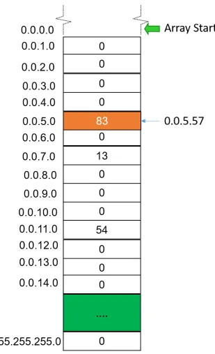
We simply use an array to implement the hash table (see Figure 4.1); such

simple choice of data structure would allow the implementation of the algorithm regardless of the programming language. This array has 224 _{entries. We split}

the IP space to buckets of length 256, or prefixes of size 24. Each element stores the reputation of a corresponding/24 Net block. The corresponding element of a Net block can be retrieved by adding an index to the the start of the array address. The index is the result of dividing IP address with0xff. For instance, the reputation of 0.0.5.57 IP is stored in the 6 element of the array. For the /24 entries that we haven’t recorded any malicious activity, we store 0. This value is logically correct since based on historical records, there is 0 chance that an IP from this space exposes malicious activity.

4.1.2

Initialization

In order to materialize the Indexing Search algorithm, we first need to initialize a byte array of size 224_{with the corresponding probabilities of the/24 prefixes.}

Since the reputation database may contain shorter net block entries than/24,

4.1. INDEXING SEARCH ALGORITHM (ISA) 37

38CHAPTER 4. AGGREGATED REPUTATION LOOKUP IMPLEMENTATION

the footprint, however, increases as a result.

Algorithm 1: Covert a reputation database with entries’ prefix larger than 24 to 24

Data: Three arrays of NetIDs, Lengths and Probabilities

Result: Two derived lists of Fixed NetIDs and Fixed Probabilities Fixed NetIDs:=List();

Fixed Probabilities:=List();

fori:=1 to len(NetIDs) do

start NetID = NetID[i];

Num Of Prefixes = 224−Lengths[i] ;

forj:=1 to Num Of Prefixes do

m:= (j-1) * 256;

Fixed NetID := start NetID + m; Fixed NetIDs.append(Fixed NetID); Fixed Probabilities.append(Probabilities[i]);

end end

Algorithm 2:Initialize the Indexing Array with the corresponding prob-abilities

Data: Two lists of Fixed NetIDs and Fixed Probabilities

Result: Array Indexed NetIDs with corresponding probabilities Indexed NetIDs := Byte[224_];

fori:=1 to len(Indexed NetIDs) do

Indexed NetIDs := 0;

end

forj:=1 to len(Fixed NetIDs) do

PrefixID := Fixed NetID.ElementAt(j); Index := PrefixID/256;

Indexed NetIDs[Index] := Fixed Probabilities.ElementAt(j);

end

4.1.3

Searching

Using the Indexed array, the reputation of any IP address can be easily fetched by converting it to an index to its reputation. The reputation searching is illustrated in Algorithm3.

Algorithm 3:Initialize the Indexing Array with the corresponding prob-abilities

Data: Indexed NetIDs and IP

Result: Reputation Index := IP / 256 ;

4.2. BINARY SEARCH ALGORITHM 39

4.2

Binary Search Algorithm

For the second algorithm, we employ the classic Binary Search algorithm with a small adjustment. In order to employ Binary Search, we initialize an array with the start and the end addresses of every net block. The difference with the classic Binary Search Algorithm is that we don’t store a value but abstractly a range start and end address in the array. Then, in order to find a reputation, we find the array index of the corresponding prefix starting address of an input IP, and use it as an index to the probabilities array.

4.2.1

Data structure

Our data structure for this algorithm is a sorted array. This sorted array con-tains the initial and end addresses of every net block for which we have a reputa-tion. Our goal in the binary search implementation is not to find a value in the array but to find the relevant range for an IP address. For instance, given a set of{1.1.1.0/24,1.1.24.0/24,2.16.196.0/20}, our data structure to start the search is an array of [16843008,16843520,16848896,16849152,34653184,34654208]

4.2.2

Initialization

To build our data structure, we need to load all the initial and end addresses of a net block in a sorted array. To achieve this, we read each NetID and the corresponding lengths from a sorted array, and according to its prefix size, we compute the end address of the prefix. We store the initial addresses at Odd indexes and the end addresses at even indexes of the array. It goes unsaid that this array is as twice as the initial NetID array. Algorithm 4 illustrates the process to construct our data structure.

Algorithm 4:Initializing range array data structure for the binary search

Data: Sorted NetIDs and NetID Lengths

Result: Sorted range array R NetIDs R NetIDs size := 2 * len(NetIDs) ; R NetIDs = Byte[R NetIDs size] ;

fori:=1 to len(NetIDs)do

odd := NetIDs[i];

even := odd + 232−N etID Lengths[i] _;

R NetIDs[2i-1] := odd; R NetIDs[2i] := even;

end

4.2.3

Searching

40CHAPTER 4. AGGREGATED REPUTATION LOOKUP IMPLEMENTATION

of the IP address in our database, then the IP address value falls between an odd (lower band) and an even (higher band) value in our data structure. Otherwise, the IP address value falls between an even (lower band) and an odd (higher band) value. Following the example we presented in the begin-ning of this section, the result for searching 1.1.25.53 must return 0. Looking at [16843008,16843520,16848896,16849152,34653184,34654208], we learn that 16849205, integer value of 1.1.25.53, falls between element 4 and 5 of the array. Since the lower band, 4, is even we return 0. Algorithm5illustrates our binary search algorithm.

Algorithm 5: Binary search algorithm based on our data structure

Data: R NetIDs, Probabilities and IP

Result: Reputation low := 1 ;

high = len(R NetIDs) ;

while low + 1<high do

middle :=dlow+₂highe;

if R NetIDs[middle]>=IP then

high := m;

else

low := m;

end end

if low%=1 then

index :=blow

2 c+ 1 ;

Reputation := R NetIDs[index];

else

Reputation := 0;

end

4.3

Summary

Chapter 5

Data Collection

Methodology

In this chapter, we explain what dataset we use for our analysis. Our data comes from Redsocks company that is a cyber security solution provider in the Netherlands. The data that they shared with us contains Indicator of Com-promise used for malicious detection from network traffic. A majority of the data identifies command and control servers and also bots. We process the raw data that we receive and build a dataset of IP prefixes with an assigned score showing the number of malicious IP addresses within that prefix. In the rest of this chapter, in Section 5.1, we explain in detail what our raw dataset from Redsocks Security (RS) contains. In Section5.2, we discuss the structure of the prefix dataset we would generate from raw data. In Section5.3, we present our preprocessing steps on the raw data to construct the prefix dataset we will use later for experimental analysis. In section5.4, we give some statistics about our prepared prefix dataset.

5.1

Redsocks Raw Dataset

Redsocks Security(RS) collects Indicators Of Compromise (IOC) on a daily basis. These IOCs are used for behavioral detection of malicious activity. RS gave us access to this database for a period of 1 month starting from 2017-04-18. Since they store IOCs with a timestamp, we fetch only the IOCs that are collected within the aforementioned period. The number of indicators for four weeks of data collection that we have are reported in Table 5.1. These values report the indicators from all types e.g. file hash, URL etc. In Section5.3, we explain how we process these indicators and extract the data we need.