A New Branch and Bound Method for Solving
Sum of Linear Ratios Problem
Chun-Feng Wang, and Xin-Yue Chu
Abstract—For globally solving sum of linear ratios problem (SLRP), this paper presents a new branch-and-bound method. In this method, a new linear relaxation technique is proposed firstly; then, the initial problem SLRP is solved by a sequence of linear programming problems. Meanwhile, to improve the convergence speed of our algorithm, two accelerating techniques are presented. The proposed algorithm is proved to be conver-gent, and some experiments are provided to show its feasibility and efficiency.
Index Terms—Linear relaxation; Global optimization; Sum of linear ratios; Accelerating technique; Branch and bound.
I. INTRODUCTION
T
HIS paper considers the following sum of linear ratios problem (SLRP):SLRP
v= min Φ(x) = p
∑
i=1
δi(x)
θi(x)
s.t. Ax≤b,
where p ≥ 2, A ∈ Rm×n, b ∈ Rm are arbitrary real numbers, δi(x) =
n
∑
j=1
cijxj +di, θi(x) = n
∑
j=1
eijxj+fi
are affine functions, D ={x∈ Rn | Ax≤b} is bounded
withintD̸=∅, and for ∀x∈D,δi(x)≥0, θi(x)̸= 0, i= 1,· · ·, p. In fact, if we use the method of [1] to preprocess problem SLRP, we also only requestθi(x)̸= 0, i= 1,· · ·, p. Among fractional programming, the problem SLRP is a special class of optimization problems. Since its initial development, it has attracted the interest of practitioners and researchers for many years. There are two main reasons. One reason is that it frequently appears in a wide variety of applications, such as financial optimization [2], portfolio op-timization [3,4], microeconomics [5], plant layout design [6], transportation problems [7], layered manufacturing problems [8,9], and so on. Another reason is that, it is well-known the problem SLRP is NP-hard [10,11], that is, it generally posses multiple local optima, many of which fail to be globally optimal.
During the past years, many algorithms have been devel-oped to solve special cases of problem SLRP. For example, for x∈D, under the assumption thatδi(x)≥0, θi(x)>0, by using variable transformation, Charnes and Cooper [12]
Manuscript received Feb. 26, 2017. This paper is supported by the Na-tional Natural Science Foundation of China (U1404105), the Key Scientific and Technological Project of Henan Province(142102210058); the Youth Science Foundation of Henan Normal University(2013qk02); Henan Normal University National Research Project to Cultivate the Funded Projects (01016400105).
Chun-Feng Wang is with College of Mathematics and Information Science, Henan Normal University,Xinxiang, 453007, PR China; Henan Engineering Laboratory for Big Data Statistical Analysis and Optimal Control, School of Mathematics and Information Sciences, Henan Normal University e-mail:[email protected].
Xin-Yue Chu is with College of Mathematics and Information Science, Henan Normal University, Xinxiang, 453007, PR China.
put forward an efficient elementary simplex method with
p = 1. Based on the work of [12], Konno et al. [13] proposed a similar parametric elementary simplex method withp= 2, which can be used to solve large scale problem. When p = 3, Konno and Abe [14] developed a heuristic algorithm. When p ≥ 3, by using the characteristics of exponential and logarithmic functions, Wang et al. [15] presented a double linearization technique. By using an equivalent transformation and a linearization technique, Shen and Wang [16] proposed a branch and bound algorithm for solving a sum of linear ratios problem with coefficients. Through solving an equivalent concave minimum problem of the original problem, Benson [17] put forward a new branch and bound algorithm. Depetrini and Locatelli [18] proposed a fully polynomial time approximate scheme (FPTAS) for the case wherepis fixed. Through using suitable transformation, Benson [19] proposed a method, which has a potential to solve SLRP by some well known techniques. By using the theory of monotonic optimization, Hoaiphuong and Tuy [20] presented a unified method to solve a wider class of fractional programming problems. Under the assumption that δi(x) ≥ 0, θi(x) ̸= 0, Ji et al. [21] developed a branch and bound algorithm. Under the assumption that
θi(x)>0, Carlsson and Shi [22] proposed a linear relaxation
algorithm for solving the sum-of-linear-ratios problem with lower dimension. Under the assumption thatθi(x)̸= 0, three
global optimization algorithms were developed [1,23,24]. In the case thatδi(x)andθi(x)are nonlinear functions, several
algorithms have been proposed [25-27].
The purpose of this paper is to develop a reliable and effective method for globally solving problem SLRP with lower dimension. In this method, firstly, by utilizing the char-acteristic of the problem SLRP, we present a new lineariza-tion technique, which can be embedded within a branch-and-bound algorithm. After that, two accelerating techniques are presented, which can be used to improve the convergence speed of our algorithm. Finally, numerical experiments show that the proposed algorithm is feasible and effective, and the computational advantages are demonstrated. Compared with [15,17,22], the model considered in this paper has a more general form; compared with [1,24], our algorithm is easier to implement, and does not need to add new variables and constraints.
This paper is organized as follows. In Section 2, the new linear relaxation technique is presented, which can be used to obtain the relaxed linear program (RLP) for problem SLRP. In order to improve the convergence speed of our algorithm, two accelerating techniques are presented in Section 3. In Section 4, the global optimization algorithm is described, and the convergence of this algorithm is established. Numerical results are reported to show the feasibility and efficiency of our algorithm in Section 5.
IAENG International Journal of Applied Mathematics, 47:3, IJAM_47_3_06
II. RELAXED LINEAR PROGRAM(RLP)
In problem SLRP, for ∀x∈ D, sinceθi(x) ̸= 0, by the intermediate value theorem, we haveθi(x)>0orθi(x)<0. For convenience in expression, let
I+={i|θi(x)>0, i= 1,· · ·, p},
I−={i|θi(x)<0, i= 1,· · ·, p}.
To solve problem SLRP, the principal task is the con-struction of lower bound for this problem and its partitioned subproblems. A lower bound of problem SLRP and its partitioned subproblems can be obtained by solving a relaxed linear program (RLP). For generating the problem RLP, the strategy proposed by this paper is to underestimate the objective function Φ(x)with a linear function.
Towards this end, we first solve 2n linear programming problems l0
j = min
x∈Dxj, u
0
j = max
x∈Dxj(j = 1,· · ·, n), and
construct a rectangle H0 ={x∈Rn |l0
j ≤xj ≤u0j, j= 1,· · ·, n}. Then, the problem SLRP can be rewritten as the following form:
SLRP
v= min Φ(x) = p
∑
i=1
δi(x)
θi(x)
s.t. Ax≤b, x∈H0.
Let H = {x | l ≤ x ≤ u} be the initial box H0 or
modified box as defined for some partitioned subproblem in a branch and bound scheme. Now, we demonstrate how to derive the problem RLP for problem SLRP overH.
Compute ξi = n
∑
j=1
min{cijlj, cijuj} + di, ξi = n
∑
j=1
max{cijlj, cijuj} +di, ηi = n
∑
j=1
min{eijlj, eijuj}+
fi, ηi = n
∑
j=1
max{eijlj, eijuj}+fi, obviously, we have
ξ
i ≤δi(x)≤ξi, ηi≤θi(x)≤ηi, i= 1,· · ·, p.
To derive the problem RLP of problem SLRP overH, we first consider the term δi(x)
θi(x), i= 1,· · ·, p.
Fori∈I+, sinceηini(x)−ξiθi(x)≥0, θi(x)−ηi≤0,
we have
(ηini(x)−ξiθi(x))(θi(x)−ηi)≤0,
that is
ηini(x)θi(x)−η2iδi(x)−ξ
id
2
i(x) +ξiηidi(x)≤0.
Furthermore, we have
η2iδi(x)≥ηini(x)θi(x)−ξid2i(x) +ξiηidi(x). (1)
Sinceηiη
idi(x)>0, dividing inequality (1) byηiηθi(x), we
have
δi(x)
θi(x) ≥
δi(x)
ηi − ξ
i
η2
i
θi(x) +ξi
ηi. (2)
In addition, since ηini(x)−ξiθi(x)≥ 0, θi(x)−ηi ≥ 0,
we have
(ηini(x)−ξiθi(x))(θi(x)−ηi)≥0,
that is
ηini(x)θi(x)−ηiη
ini(x)−ξid
2
i(x) +ξiηidi(x)≥0. (3)
Dividing inequality (3) byηiη
idi(x), we can obtain
δi(x)
θi(x)
≤δi(x) η
i
− ξi
ηiη
i
θi(x) +ξi
ηi. (4)
Fori∈I−, sinceη
ini(x)−ξiθi(x)≤0, θi(x)−ηi≤0,
we have
(η
ini(x)−ξiθi(x))(θi(x)−ηi)≥0,
that is
ηini(x)θi(x)−ηiηini(x)−ξid2i(x) +ξiηidi(x)≥0. (5)
Since ηiη
idi(x) <0, dividing inequality (5) by ηiηidi(x),
we have
δi(x)
θi(x) ≥
δi(x)
ηi
− ξi
ηiηi
θi(x) +
ξ
i
ηi. (6)
Meanwhile, sinceη
ini(x)−ξiθi(x)≤0, θi(x)−ηi≥0,
we can derive
(η
ini(x)−ξiθi(x))(θi(x)−ηi)≤0,
Furthermore, we get
η
ini(x)θi(x)−η
2
iδi(x)−ξid
2
i(x) +ξiηidi(x)≤0. (7)
Dividing inequality (7) byηiη
idi(x), we have
δi(x)
θi(x)
≤ δi(x) η
i
− ξi
η2
i
θi(x) +ξi
η
i
. (8)
From (2),(4),(6) and (8), we have the following relations:
Φ(x) = p
∑
i=1
δi(x)
θi(x)= ∑
i∈I+
δi(x)
θi(x)+ ∑
i∈I−
δi(x)
θi(x)
≥ ∑
i∈I+
[δi(x)
ηi − ξ
i
η2 i
θi(x) +ξi
ηi]
+ ∑
i∈I− [δi(x)
ηi − ξ
i
ηiη
i
θi(x) +ξi
η
i
] = Φl(x),
Φ(x) = p
∑
i=1
δi(x)
θi(x) = ∑
i∈I+
δi(x)
θi(x)+ ∑
i∈I−
δi(x)
θi(x)
≤ ∑
i∈I+
[δi(x)
η
i − ξi
ηiη
i
θi(x) +ξi
ηi]
+ ∑
i∈I− [δi(x)
η
i −
ξ
i
η2 i
θi(x) +ξi
η
i
] = Φu(x),
From the above discussion, the following relaxed linear program (RLP) can be established as follows:
RLP
min Φl(x) s.t. Ax≤b,
x∈H.
This problem provides a lower bound for the optimal value of problem SLRP overH.
Theorem 1 For all x ∈ H, let ∆x = u−l, consid-er the functions Φl(x), Φ(x) and Φu(x). Then, we have
lim
∆x→0(Φ(x)−Φ
l(x)) = lim
∆x→0(Φ
u(x)−Φ(x))→0.
IAENG International Journal of Applied Mathematics, 47:3, IJAM_47_3_06
Proof We first prove lim
∆x→0(Φ(x)−Φ
l(x))→0. By the
definitions Φ(x)andΦl(x), we have
|Φ(x)−Φl(x)| =| ∑
i∈I+
[(δi(x)
θi(x)−(
δi(x)
ηi − ξ
i
η2 i
θi(x) + ξ
i
ηi)]
+ ∑
i∈I−
[δi(x)
θi(x)−(
δi(x)
ηi −
ξ
i
ηiηiθi(x) +
ξ i η i )]| ≤| ∑
i∈I+
[(δi(x)
θi(x)−(
δi(x)
ηi − ξ
i
η2 i
θi(x) + ξ
i
ηi)]|
+| ∑
i∈I− [δi(x)
θi(x)−(
δi(x)
ηi − ξ
i
ηiη
i
θi(x) +ξi
η
i
)]|
≤ ∑
i∈I+
[|δi(x)(θ1
i(x)−
1
ηi)|+| ξ
i
ηi( θi(x)
ηi −1)|]
+ ∑
i∈I−
[|δi(x)(θ1
i(x)−
1
ηi)|+| ξ
i
η
i
(θi(x)
ηi −1)|]
= ∑
i∈I+
[|δi(x) ηi−θi(x)
ηidi(x) |+|
ξ
i
ηi
θi(x)−ηi
ηi |]
+ ∑
i∈I−
[|δi(x) ηi−θi(x)
ηidi(x) |+|
ξ
i
η
i
θi(x)−ηi
ηi |]
≤ ∑
i∈I+
[ξiηi−ηi
ηiη
i
+ξi
ηi ηi−η
i
ηi ] +
∑
i∈I−
[ξiηi−ηi
ηiη
i
+ ξi
|η
i|
ηi−η
i
|ηi| ]
= ∑
i∈I+
[ξiηi−ηi
ηiη
i
+ξi
ηi ηi−η
i
ηi ] +
∑
i∈I− [ξiηi−ηi
ηiη
i
+ ξi
|η
i|
ηi−η
i
|ηi| ].
By the definitions of η
i and ηi, we know that, ∆s =
ηi−η
i→0as∆x→0. From the above inequality, we have lim
∆x→0(Φ(x)−Φ
l(x)) = 0.
Similarly, we can prove lim
∆x→0(Φ
u(x)−Φ(x)) = 0, and
the proof is complete.
From Theorem 1, it follows that Φl(x) and Φu(x) will
approximate the function Φ(x)as ∆x→0.
III. ACCELERATING TECHNIQUES
As is well known, accelerating techniques are important for improving the convergence speed of an algorithm [26]. So, this section presents two accelerating techniques, which can be used to eliminate the region in which the global optimal solution of problem SLRP does not exist.
The accelerating techniques are derived as in the following theorems.
Theorem 2 Assume thatU Bis the current known upper bound of the optimal value v of the problem SLRP over
H ⊆H0. If there exists some indexk∈ {1,2,· · ·, n}such that αk > 0, then there is no globally optimal solution of
problem SLRP over H1; if α
k <0 for somek, then there
is no globally optimal solution of problem SLRP over H2,
where
H1= (Hj1)n×1⊆H, with Hj1=
{
Hj, j̸=k, (γk
αk, uk] ∩
Hk, j=k,
H2= (Hj2)n×1⊆H, with Hj2=
{
Hj, j̸=k,
[lk,αγkk) ∩
Hk, j=k,
αk =
∑
i∈I+
(cik
ηi − ξ
i
η2 i
eik) + ∑ i∈I−
(cik
ηi − ξ
i
ηiη
i eik),
Λ1=
∑
i∈I+
(di
ηi + ξ
i
ηi − ξ
i
η2 i
fi) + ∑ i∈I−
(di
ηi + ξ i η i − ξ i
ηiη
i fi),
γk=U B− n
∑
j=1,j̸=k
min{αjlj, αjuj} −Λ1.
proof Consider the kth component xk ofx. Fromxk∈ (γk
αk, uk], it follows that γk
αk
< xk ≤uk.
Sinceαk >0, we haveγk < αkxk. For allx∈H1, by the
above inequality and the definition ofγk, it implies that
U B−
n
∑
j=1,j̸=k
min{αjlj, αjuj} −Λ1< αkxk,
that is
U B <
n
∑
j=1,j̸=k
min{αjlj, αjuj}+αkxk+ Λ1
≤ ∑n
j=1
αjxj+ Λ1= Φl(x).
Thus, for allx∈H1, we haveΦ(x)≥Φl(x)> U B ≥v,
i.e. for allx∈H1,Φ(x)is always greater than the optimal
valuevof the problem SLRP. Therefore, there can not exist globally optimal solution of problem SLRP overH1.
For allx∈H2, if there exists somek such that αk <0,
from arguments similar to the above, it can be derived that there is no globally optimal solution of problem SLRP over
H2
Theorem 3 Assume thatLBis the current known lower bound of the optimal value v of the problem SLRP over
H ⊆H0. If there exists some index k∈ {1,2,· · ·, n} such
that βk > 0, then there is no globally optimal solution of
problem SLRP over H3; if βk <0, for somek, then there
is no globally optimal solution of problem SLRP overH4, where
H3= (Hj3)n×1⊆H, with Hj3=
{
Hj, j̸=k,
[lk,ρβkk)
∩
Hk, j=k,
H4= (Hj4)n×1⊆H, with Hj4=
{
Hj, j̸=k, (ρk
βk, uk] ∩
Hk, j=k,
βk=
∑
i∈I+
(cik
η
i −
ξ
i
ηiη
i
eik) + ∑ i∈I−
(cik
η i − ξ i η2 i
eik),
Λ2=
∑
i∈I+
(di
η
i
+ ξi
ηi − ξ
i
ηiη
i fi) +
∑
i∈I− (di
η
i
+ ξi
η i − ξ i η2 i
fi),
ρk =LB− n
∑
j=1,j̸=k
max{βjlj, βjuj} −Λ2.
proof Consider the kth component xk of x. By the
assumption and the definitions ofβk andρk, we have
lk ≤xk <
ρk
βk
.
Note thatβk >0, we have ρk > βkxk. For all x∈H3, by
the above inequality and the definition ofρk, it implies that
LB >
n
∑
j=1,j̸=k
max{βjlj, βjuj}+βkxk+ Λ2
≥ ∑n
j=1
βjxj+ Λ2= Φu(x)≥Φ(x).
Thus, for allx∈H3, we havev≥LB >Φ(x). Therefore,
there can not exist globally optimal solution of problem SLRP overH3.
For allx∈H4, if there exists some k such thatβk <0,
from arguments similar to the above, it can be derived that there is no globally optimal solution of problem SLRP over
H4
IAENG International Journal of Applied Mathematics, 47:3, IJAM_47_3_06
IV. ALGORITHM AND ITS CONVERGENCE
In this section, based on the former results, we present the branch and bound algorithm to solve problem SLRP. In order to find a global optimal solution, this method needs to solve a sequence of relaxed linear programming problems over partitioned subsets of H0.
A. Branching rule
During each iteration of the algorithm, the branching process is a critical element in guaranteeing convergence, which can be used to create a more refined partition that cannot yet be excluded from further consideration in search-ing for a global optimal solution for problem SLRP. This paper chooses a simple and standard bisection rule, which is sufficient to ensure convergence since it drives the intervals shrinking to a singleton for all the variables along any infinite branch of the branch and bound tree.
Consider any node subproblem identified by rectangle
H = {x ∈ Rn | l
j ≤ xj ≤ uj, j = 1,· · ·, n} ⊆ H0.
The branching rule is as follows:
(i) let k=argmax{uj−lj |j= 1,· · ·, n};
(ii) let πk = (lk+uk)/2;
(iii) let
H1={x∈Rn|l
j ≤xj≤uj, j̸=k, lk ≤xk ≤πk},
H2={x∈Rn|l
j ≤xj≤uj, j̸=k, πk ≤xk ≤uk}.
Through using this branching rule, the rectangle H is partitioned into two subrectangles H1 andH2.
B. Branch and bound algorithm
Based upon the results and operations given above, this subsection summarizes the basic steps of the proposed algo-rithm.
Let LB(Hk) be the optimal function value of RLP over the subrectangle H =Hk, andxk =x(Hk)be an element of the corresponding argmin.
Algorithm statement
Step 1. Choose ϵ ≥ 0. Find an optimal solution x0 =
x(H0)and the optimal valueLB(H0)for problem RLP with
H = H0. Set LB
0 = LB(H0), and U B0 = Φ(x0). If
U B0−LB0≤ϵ, then stop:x0 is an ϵ-optimal solutions of
problem SLRP. Otherwise, set Q0={H0}, F =∅, k= 1,
and go to Step 2.
Step 2. Set U Bk = U Bk−1. Subdivide Hk−1 into two
subrectangles Hk,1, Hk,2 via the branching rule. Set F =
F∪{Hk−1}.
Step 3. Set t=t+ 1. Ift >2, go to Step 5. Otherwise, continue.
Step 4. If LB(Hk,t)> U Bk, set F =F
∪
{Hk,t}, and go to Step 3. Otherwise, letU Bk = min{U Bk,Φ(xk,t)}. If
U Bk = Φ(xk,t), setxk =xk,t, go to Step 3.
Step 5.Set
F =F∪{H ∈Qk−1|U Bk≤LB(H)},
Qk={H|H∈(Qk−1
∪
{Hk,1, Hk,2}), H /∈F}.
Step 6. Set LBk = min{LB(H) | H ∈ Qk}. Let Hk
be the subrectangle which satisfies thatLBk=LB(Hk). If
U Bk−LBk≤ϵ, then stop:xk is a globalϵ-optimal solution
of problem SLRP. Otherwise, setk=k+ 1, and go to Step 2.
C. Convergence analysis
In this subsection, we give the global convergence prop-erties of the above algorithm.
Theorem 4 The above algorithm either terminates finite-ly with a globalfinite-lyϵ-optimal solution, or generates an infinite sequence{xk}of iteration such that any accumulation point is a globally optimal solution of problem SLRP.
Proof If the algorithm terminates finitely, then it ter-minates at some step k ≥ 0. Upon termination, by the algorithm, it follows that
U Bk−LBk≤ϵ. (9)
Furthermore, from Step 4 and (9), the following relation holds
Φ(xk)−LBk≤ϵ. (10)
By Section 2, we have
LBk≤v. (11)
Meanwhile, sincexkis a feasible solution of problem SLRP,
Φ(xk)≥v. (12)
From (10)-(12), it implies that
v≤Φ(xk)≤LBk+ϵ≤v+ϵ.
So,xk is a global ϵ-optimal solution of the problem SLRP overH0 in the sense that
v≤Φ(xk)≤v+ϵ.
If the algorithm terminates infinitely, then an infinite sequence{xk} will be generated. Since the feasible region
of SLRP is bounded, there exists a convergence subsequence in{xk}. Without loss of generality, this subsequence is still represented by{xk}and set lim
k→∞x
k =x∗. By the algorithm,
we have
lim
k→∞LBk ≤v. (13)
Sincex∗ is a feasible solution of problem SLRP,
v≤Φ(x∗). (14)
From (13) and (14), we have
lim
k→∞LBk ≤v≤Φ(x
∗). (15)
On the other hand, by the algorithm and the continuity of
Φl(x), we have lim
k→∞LBk= limk→∞Φ
l(xk) = Φl(x∗). (16)
By Theorem 1, we have
Φ(x∗) = Φl(x∗). (17)
Therefore, from (16) and (17), we havev = Φ(x∗), that is
x∗ is a global optimal solution of problem SLRP.
IAENG International Journal of Applied Mathematics, 47:3, IJAM_47_3_06
V. NUMERICAL EXPERIMENTS
To validate the performance of the proposed algorith-m, some examples taken from the optimization literatures [1,15,16,23,29,30] were solved. Numerical results are re-ported, and compared with that of these references. The algorithm is implemented in Matlab 7.1, and all test problems are carried out on a Pentium IV (3.06 GHZ) microcomputer. The linear relaxation programming problems are solved by using simplex method.
The results of problems 1-7 are summarized in Table I, where the following notations have been used in row headers:
[image:5.595.307.542.69.332.2]ϵ: convergence error; Iter: number of algorithm iterations. For Examples 1-7, we also used two algorithms to solve them, which are the algorithm (named Algorithm 1) proposed by this paper and the algorithm proposed by this paper but without using pruning techniques(named Algorithm 2), respectively. The comparison results are given in Table II. In Table II, T ime denotes execution time in seconds. For this test, ϵis set to1e−5.
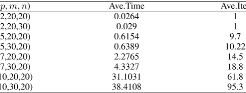
Table III summarizes our computational results of Exam-ple 8. For this test problem, ϵ is set to 1e−2. In Table II, Ave.Iter represents the average number of iterations;
Ave.Timestands for the average CPU time of the algorithm in seconds, which are obtained by randomly running our algorithm for 10 test problems.
Example 1[1]
max 0.9×−x1+ 2x2+ 2 3x1−4x2+ 5
+ (−0.1)× 4x1−3x2+ 4
−2x1+x2+ 3
s.t. x1+x2≤1.5,
x1−x2≤0,
0≤x1≤1, 0≤x2≤1.
Example 2[1,15,30]
max 4x1+ 3x2+ 3x3+ 50 3x2+ 3x3+ 50
+ 3x1+ 4x3+ 50 4x1+ 4x2+ 5x3+ 50
+x1+ 2x2+ 5x3+ 50
x1+ 5x2+ 5x3+ 50
+x1+ 2x2+ 4x3+ 50 5x2+ 4x3+ 50
s.t. 2x1+x2+ 5x3≤10,
x1+ 6x2+ 3x3≤10,
5x1+ 9x2+ 2x3≤10,
9x1+ 7x2+ 3x3≤10,
x1≥0, x2≥0, x3≥0, x4≥0.
Example 3[30]
min −x1+ 2x2+ 2 3x1−4x2+ 5
+ 4x1−3x2+ 4
−2x1+x2+ 3
s.t. x1+x2≤1.5,
x1−x2≤0,
0≤x1≤1, 0≤x2≤1.
Example 4[29,30]
max 3x1+ 5x2+ 3x3+ 50 3x1+ 4x2+ 5x3+ 50
+ 3x1+ 4x2+ 50 4x1+ 3x2+ 2x3+ 50
+4x1+ 2x2+ 4x3+ 50 5x1+ 4x2+ 3x3+ 50
s.t. 6x1+ 3x2+ 3x3≤10,
10x1+ 3x2+ 8x3≤10,
x1≥0, x2≥0, x3≥0.
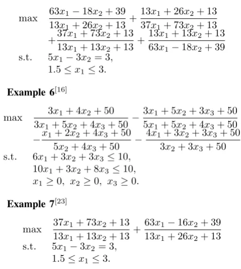
Example 5[16]
max 63x1−18x2+ 39 13x1+ 26x2+ 13
+13x1+ 26x2+ 13 37x1+ 73x2+ 13
+37x1+ 73x2+ 13 13x1+ 13x2+ 13
+13x1+ 13x2+ 13 63x1−18x2+ 39
s.t. 5x1−3x2= 3,
1.5≤x1≤3.
Example 6[16]
max 3x1+ 4x2+ 50 3x1+ 5x2+ 4x3+ 50
−3x1+ 5x2+ 3x3+ 50
5x1+ 5x2+ 4x3+ 50
−x1+ 2x2+ 4x3+ 50
5x2+ 4x3+ 50
−4x1+ 3x2+ 3x3+ 50
3x2+ 3x3+ 50
s.t. 6x1+ 3x2+ 3x3≤10,
10x1+ 3x2+ 8x3≤10,
x1≥0, x2≥0, x3≥0.
Example 7[23]
max 37x1+ 73x2+ 13 13x1+ 13x2+ 13
+63x1−16x2+ 39 13x1+ 26x2+ 13
s.t. 5x1−3x2= 3,
1.5≤x1≤3.
TABLE I: Computational results of Examples 1-7
Example ϵ Methods Optimal solution Optimal value Iter
1 1e-9 [1] (0.0, 1.0) 3.575 1
1e-9 ours (0.0, 1.0) 3.575 1
2 1e-9 [1] (1.1111, 0.0, 0.0) 4.0907 1289 1e-6 [15] (1.1111, 1.365e-5, 1.351e-5) 4.081481 39 1e-5 [30] (0.0013, 0.0, 0.0) 4.087412 1640 1e-9 ours (1.1111, 0.0, 0.0) 4.0907 18 3 1e-8 [30] (0.0, 0.283935547) 1.623183358 71 1e-8 ours (0.0, 0.283935547) 1.623183358 47 4 1e-5 [29] (0.0, 1.6725, 0.0) 3.0009 1033
1e-8 [30] (0.0, 3.3333, 0.0) 3.00292 119 1e-8 ours (0.0, 3.3333, 0.0) 3.00292 50
5 1e-6 [16] (3.0, 4.0) 3.2917 9
1e-6 ours (3.0, 4.0) 3.2917 8
6 1e-6 [16] (-1.838e-16, 3.3333, 0.0) 1.9 8 1e-6 ours (0.0, 3.3333, 0.0) 1.9 6
7 1e-4 [23] (3.0, 4.0) 5.0 32
[image:5.595.308.557.373.521.2]1e-4 ours (3.0, 4.0) 5.0 17
TABLE II: Computational results of Algorithm 1 and Algo-rithm 2 for Examples 1-7
Example Methods Optimal solution Optimal value Iter T ime
1 Algorithm 1 (0.0, 1.0) 3.575 1 0.016 Algorithm 2 (0.0, 1.0) 3.575 1 0.016 2 Algorithm 1 (1.1111, 0.0, 0.0) 4.0907 9 0.281 Algorithm 2 (1.1111, 0.0, 0.0) 4.081481 20 0.672 3 Algorithm 1 (0.0, 0.283935547) 1.623183358 31 1.0
Algorithm 2 (0.0, 0.283935547) 1.623183358 50 1.719 4 Algorithm 1 (0.0, 3.3333, 0.0) 3.0009 40 1.328 Algorithm 2 (0.0, 3.3333, 0.0) 3.00292 77 2.562 5 Algorithm 1 (3.0, 4.0) 3.2917 8 0.187 Algorithm 2 (3.0, 4.0) 3.2917 10 0.203 6 Algorithm 1 (0, 3.3333, 0.0) 1.9 5 0.172 Algorithm 2 (0.0, 3.3333, 0.0) 1.9 28 0.922
7 Algorithm 1 (3.0, 4.0) 5.0 19 0.568
Algorithm 2 (3.0, 4.0) 5.0 35 1.253
From Table I, it can be seen that, for Examples 1-7, our algorithm can determine the global optimal solution effectively than that of the references [1,15,16,23,29,30].
The comparison results of Table 2 show that the pruning techniques are very good at improving the convergence speed of our algorithm.
IAENG International Journal of Applied Mathematics, 47:3, IJAM_47_3_06
[image:5.595.50.286.380.805.2]Example 8
min p
∑
i=1
n
∑
j=1
cijxj+di
n
∑
j=1
eijxj+fi
s.t. x∈D={x∈Rn|Ax≤b},
where the elements of the matrixA∈Rm×n, c
ij, ei,j∈R
are randomly generated in the interval [0,1]. All constant terms of denominators and numerators are the same number, which randomly generated in [50,100]. The elements ofb∈ Rmare equal to 1. This agrees with the way random numbers are generated in [22].
From Table III, the computational results show that our algorithm performs well on the test problems, and can solve them in a reasonable amount of time.
[image:6.595.52.294.284.376.2]The results in Tables I-III show that our algorithm is both feasible and efficient.
TABLE III: Computational results of Example 8
(p, m, n) Ave.Time Ave.Iter
(2,20,20) 0.0264 1
(2,20,30) 0.029 1
(5,20,20) 0.6154 9.7
(5,30,20) 0.6389 10.22
(7,20,20) 2.2765 14.5
(7,30,20) 4.3327 18.8
(10,20,20) 31.1031 61.8
(10,30,20) 38.4108 95.3
REFERENCES
[1] H.W. Jiao , S.Y. Liu, ”A practicable branchand bound algorithm forsum of linear ratios problem,”European Journal of Operational Research, vol. 243, no. 3, pp 723-730, 2015.
[2] C.D. Maranas, I.P. Androulakis, C.A. Floudas, A.J. Berger, J.M. Mulvey, ”Solving long-term financial planning problems via global optimization,”Journal of Economic Dynamics and Control, vol. 21, no. 8-9, pp 1405-1425, 1997.
[3] H.M. Markowitz, Portfolio Selection, 2nd edition,Basil Blackwell Inc., Oxford,1991.
[4] T. Hasuike, H. Katagiri, ”Sensitivity analysis for random fuzzy portfolio selection model with investor′s subjectivity,” IAENG International Journal of Applied Mathematics, vol. 40, no. 3, pp 185-189, 2010. [5] J.M. Henderson, R.E. Quandt, Microeconomic Theory, 2n dedition, Mc
Graw-Hill, New York, 1971.
[6] I. Quesada, I.E. Grossmann, Alternative bounding approximations for the global optimization of various engineering design problems, in: Global Optimization in Engineering Design, Nonconvex Optimization and Its Applications, vol. 9, Kluwer AcademicPublishers, Norwell, MA, 1996.
[7] Y. Almogy, O. Levin, Parametric analysis of a multi-stage stochastic shipping problem, in: Lawrenle, J.(ed) Operational Research ’69, Tavi-stock Publications, London, 1970.
[8] J. Majihi, R. Janardan, et al, ”On some geometric optimization problems in layered manufacturing,”Computational Geometry, vol. 12, no. 3-4, pp 219-239, 1999.
[9] X.J. Wang, S.H. Choi, ”Optimisation of Stochastic Multi-item Manu-facturing for Shareholder Wealth Maximisation,”Engineering Letters, vol. 21, no. 3, pp 127-136, 2013.
[10] R.W. Freund, F. Jarre, ”Solving the sum-of-ratios problem by an interior-point method,”Journal of Global Optimization, vol. 19, no. 1, pp 83-102, 2001.
[11] T. Matsui, ”NP-hardness of linear multiplicative programming and related problems,”Journal of Global Optimization, vol. 9, no.2 pp 113-119, 1996.
[12] A. Charnes, W.W. Cooper, ”Programming with linear fractional func-tionals,”Naval Research Logistick Quarterly, vol. 9, no. 3-4, pp 181-186, 1962.
[13] H. Konno, Y. Yajima, T. Maktkui, ”Parametric simples algorithms for solving a special class of nonconvex minimization problems,”Journal of Global Optimization, vol. 1, no. 1, pp 65-81, 1991.
[14] H. Konno, N. Abe, ”Minimization of the sum of three linear fractional functions,”Journal of Global Optimization, vol. 15, no. 4, pp 419-432, 1999.
[15] Y.J. Wang, P.P. Shen, Z.A. Liang, ”A branch-and-bound algorithm to globally solve the sum of several linear ratios,”Applied Mathematics and Computation, vol. 168. no. 1, pp 89-101, 2005.
[16] P.P. Shen, C.F. Wang, ”Global optimization for sum of linear ratios problem with coeicients,”Applied Mathematics and Computation, vol. 176, no. 1, pp 219-229, 2006.
[17] H.P. Benson, ”Solving sum of ratios fractional programs via concave minimization,” Journal of Optimization Theory and Application, vol. 135, no. 1, pp 1-17, 2007.
[18] D. Depetrini, M. Locatelli, ”Approximation of linear fractional-multiplicative problems,”Mathematical Programming, vol. 128, no. 1, pp 437-443, 2011.
[19] H.P. Benson, ”On the global optimization of sums of linear fractional functions over a convex set,” Journal of Optimization Theory and Application, vol. 121, no. 1, pp 19-39, 2004.
[20] N.T. Hoaiphuong, H. Tuy, ”A unified monotonic approach to gener-alized linear fractional programming,”Journal of Global Optimization, vol. 26, no. 3, pp 229-259, 2003.
[21] Y. Ji, K.C. Zhang, S.J. Qu, ”A deterministic global optimization algorithm,” Applied Mathematics and Computation, vol. 185, no. 1, pp 382-387, 2007.
[22] J.G. Carlsson, J.M. Shi, ”A linear relaxation algorithm for solving the sum-of-linear-ratios problem with lower dimension,” Operations Research Letter, vol. 41, no. 4, pp 381-389, 2013.
[23] C.F. Wang, P.P. Shen, ”A global optimization algorithm for linear fractional programming,”Applied Mathematics and Computation, vol. 204, no. 1, pp 281-287, 2008.
[24] H.P. Benson, ”A simplicial branch and bound duality-bounds algorithm for the linear sum-of-ratios problem,”European Journal of Operational Research, vol. 182, no. 2, pp 597-611, 2007.
[25] L. Gao, S.K. Mishra, J. Shi. ”An extension of branch-and-bound algorithm for solving sum-of-nonlinear-ratios problem,” Optimization Letters, vol. 6, no. 2, pp 221-230, 2012.
[26] H.W. Jiao, Z. Wang, Y.Q. Chen, ”Global optimization algorithm for sum of generalized polynomial ratios problem,”Applied Mathematical Modelling, vol. 37, no. 1-2, pp 187-197, 2013.
[27] M. Jaberipour, E. Khorram, ”Solving the sum-of-ratios problems by a harmony search algorithm,”Journal of Computational and Applied Mathematics, vol. 234, no. 3, pp 733-742, 2010.
[28] C.F. Wang, S.Y. Liu, ”A new linearization method for generalized lin-ear multiplicative programming,”Computers and Operations Research, vol. 38, no. 7, pp 1008-1013, 2011.
[29] Y.G. Pei, D.T. Zhu, ”Global optimization method for maximizing the sum of difference of convex functions ratios over nonconvex region,”
Journal of Applied Mathematics and Computing, vol. 41, no. 1, pp 153-169, 2013.
[30] H.W. Jiao, ”A branch and bound algorithm for globally solving a class of nonconvex programming problems,” Nonlinear Analysis: Theory, Methods and Applications, vol. 70, no. 2, pp 1113-1123, 2009.