Estimating the Undercoverage of a Sampling Frame due to Reporting Delays

Abstract

One of the imperfections of a sampling frame is miscoverage caused by delays in recording real- life events that change the eligibility of population units. For example, new units generally appear on the frame some time after they came into existence and units that have ceased to exist are not removed from the frame immediately. We provide methodology for predicting the undercoverage due to delays in reporting new units. The approach presented here is novel in a business survey context, and is equally applicable to overcoverage due to delays in reporting the closure of units. As a special case, we also predict the number of new-born units per month. The methodology is applied to the principal business register in the UK, maintained by the Office for National Statistics.

SSRC Methodology Working Paper M03/08

Estimating the Undercove rage of a Sampling

Frame due to Reporting

Delays

Estimating the Undercoverage of a Sampling Frame

due to Reporting Delays

Dan Hedlin1_{, Trevor Fenton}2_{, John W. McDonald}1_{, Mark Pont}2_{, and Suojin Wang}3

Abstract

One of the imperfections of a sampling frame is miscoverage caused by delays in recording

real- life events that change the eligibility of population units. For example, new units

generally appear on the frame some time after they came into existence and units that have

ceased to exist are not removed from the frame immediately. We provide methodology for

predicting the undercoverage due to delays in reporting new units. The approach presented

here is novel in a business survey context, and is equally applicable to overcoverage due to

delays in reporting the closure of units. As a special case, we also predict the number of

new-born units per month. The methodology is applied to the principal business register in

the UK, maintained by the Office for National Statistics.

Keywords: Frame quality, births and deaths, birth lags, right-truncated data.

Acknowledgements: This work was partly supported by funding from Eurostat, the

Statistical Office of the European Communities. Wang’s research was also supported by the

U.S. National Cancer Institute (CA 57030).

1. Introduction

Most sample surveys draw their samples from a frame. More often than not, part of the

target population is not accessible from the frame; the survey will suffer from

undercoverage. A reporting delay or, using an equivalent term, a birth lag is defined as the

time from birth (for a frame of businesses, the date when the business began to trade) to

frame introduction (the date when the business came onto the sampling frame). Conversely,

1

University of Southampton, Department of Social Statistics, Southampton SO17 1BJ, UK. e-mail addresses :

[email protected] and [email protected]

2 _{Office for National Statistics, Cardiff Road, Newport N10 8XG, UK, e -mail addresses:}

[email protected] and [email protected]

3

the death lag, causing overcoverage, is the time between cessation of activity (death) and the

business being removed from the frame. It is believed that for the business surveys run by

the Office for National Statistics (ONS) in the UK, reporting delays are the most important

source of undercoverage.

Most information on births and deaths is updated as soon as it is received in the ONS.

However, some information relating to births and deaths is held back pending further

information or investigation. When the size information indicates that the new unit has a

workforce numbering twenty or more, and the unit cannot be matched against existing frame

units, the recording of the unit is further delayed pending proving of the information about

the unit. On average this adds about two months to the reporting delay these businesses

would have otherwise. The lengths of birth lags form a highly skewed distribution. Some

businesses report to the relevant authority in the UK as soon as they are set up, resulting in

short lags. Others may have been operating for years below the level of annual turnover

above which registration is compulsory, i.e. before their growth necessitates their

registration. In these cases the lag may be very long indeed. Some businesses report to an

administrative body in advance of their launch, sometimes resulting in a negative birth lag.

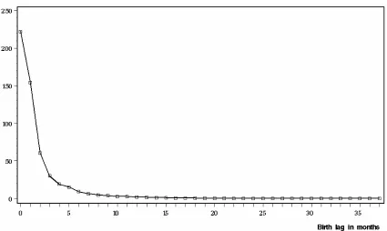
Figure 1 shows the distribution of births over non- negative birth lags. The vast majority of

new businesses (85%) have been registered on the ONS frame within four months of their

birth. About 10% have birth lags longer than five months.

The aim of the paper is to devise a method for estimating the undercoverage that is caused

by birth lags. The approach is to fit a generalised linear model to historical frame records for

which both birth dates and reporting delays have been recorded. The model will then be

used for predicting forthcoming numbers and lags. While we could accommodate economic

cycles that have been observed in historical data, we have not attempted to do so as the

available usable data relate only to the period January 1995 – March 1998. Businesses that

never come onto the frame, for example, very small businesses or businesses operating

entirely on the black market, are ignored, as are businesses that die before they appear on the

Figure 1. Number of observed births (in thousands) against birth lag (months).

In general at the ONS it is not possible to tell whether a dead business has been closed

because of a genuine death or because it has been part of a merger, takeover etc. Information

that precedes the start of a business in legal terms is not recorded. The net number of births

may therefore be more interesting than the gross total. Deaths are reported through the same

administrative bodies and the resulting reporting delays will be similar to birth lags,

although they tend to be longer. The net number of births can be estimated as the difference

between the predicted gross numbers of births and deaths. While we focus on birth lags, the

same methods could be applied to death lags.

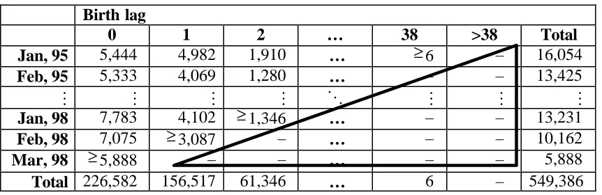
Table 1 indicates the birth lag distribution for businesses born between 1 January 1995 and

22 March 1998. The rows of the table represent the numbers of businesses that were born in

each month. We refer to the month a business started operating as its birth month. The

columns are birth lags measured in mo nths calculated as the number of complete months

(successive periods of 30.4 days) between birth and frame introduction.

The business registers of the ONS and the former Employment Department were merged in

1993 to create the Inter-Departmental Business Register (IDBR). Before 1995 the IDBR was

in a state of considerable flux as data from the two previous registers were being matched

The administrative sources that the IDBR is built upon are two government departments:

HM Customs and Excise and Inland Revenue. HM Customs and Excise provides

information relating to Value Added Tax (VAT)-registered legal units daily (weekly up to

1999). These indicate new registrations, and any traders that have deregistered. Inland

Revenue provides a file of all Pay As You Earn (PAYE) employer records each quarter. In

the PAYE scheme employers pay the employees’ income tax and national insurance

contributions. From these notifications, new registrations and deregistrations can be detected

by comparison with the file from the previous quarter.

Because the ONS is not notified continuously, frame introductions tend to be clustered in

time. The total number of businesses on the IDBR in 1998 was about 1.8 million (in

addition to the data analysed here there was a large number of businesses that went

unchanged through a period starting in 1995 and ending in February 1998).

With the observation window spanning the period January 1995 – March 1998 the longest

observable birth lag is 38 months. The count of the rightmost cell in the first row of Table 1

is unobservable (unless we gain access to data that go beyond the final date in the data

currently available). Adhering to common terminology, cells with unknown counts are

referred to as structural zeroes (see e.g. Agresti 1990); their unknown counts are represented

in Table 1 with dashes. The term structural zero is conventional but in this case

‘unobservable counts’ might have been more telling. With structural zeroes, the table is an

incomplete contingency table. The rightmost diagonal of the upper triangle containing

observed counts is partially unobservable.

Another way of expressing the fact that we cannot observe new businesses that have not yet

been introduced on the sampling frame is to say that the data are right-truncated. The

problem of estimating the undercoverage due to birth lags is equivalent to estimating the

number of businesses that have been subjected to right-truncation.

On 31 March 1998, the undercoverage is the sum of the unknown counts in the lower

triangle of Table 1. As a special case, the row totals can be predicted; they correspond to the

number of births per month. Note that it is the column sums of Table 1, excluding partially

Table 1.Number of observed births per lag (in months) and birth month. Partially

unobservable cell counts are indicated with a ≥ symbol, totally unobserved cell counts

with a dash.

Birth lag

0 1 2 … 38 >38 Total

Jan, 95 5,444 4,982 1,910 … ≥6 – 16,054

Feb, 95 5,333 4,069 1,280 … – – 13,425

M M M M O M M M

Jan, 98 7,783 4,102 ≥1,346 … – – 13,231

Feb, 98 7,075 ≥3,087 – … – – 10,162

Mar, 98 ≥5,888 – – … – – 5,888

Total 226,582 156,517 61,346 … 6 – 549,386

There is surprisingly little literature on reporting-delay induced undercoverage of a frame

used for sample surveys, considering the importance of the problem and the fact that there is

research on similar issues in other areas. The approach presented here to estimate the

number of unobservable businesses is akin to and was inspired by estimation of the

incidence of cases of AIDS in the presence of reporting delays, see Wang (1992), Sellero et

al. (1996) and references therein. Our application is different; we have a very large dataset

and a large contingency table. There is also a structure to our data that makes assumptions

that are common in AIDS research less appealing.

An extension to the problem of predicting the population size is to predict the population

total of some variable. Most businesses in transition between start and frame introduction

are part of the target population and hence their absence from the sampling frame will result

in a negative bias in estimated totals if these are based solely on samples from the frame. We

propose a method of estimating this bias. A similar estimation problem is addressed in

actuarial science. Insurance companies need to estimate the net sum of claims that have yet

to be settled; see, e.g., Haberman and Renshaw (1996).

Section 2 explores the data behind the incomplete contingenc y table and the table itself. In

Sections 3 and 4 Poisson regression models are fitted to the upper triangle of Table 1 to

predict the unobservable cell counts in the lower triangle. In Section 5 the precision of each

model is assessed by a cross-validatio n type of study. Section 6 addresses the problem of

bias in estimates of the total in the presence of reporting delays. The paper concludes with a

2. Exploring the data

It is useful to start with an in-depth data exploration. In addition to measuring the overall

length of birth lags, we have also examined lags by industry classified by the Standard

Industrial Classification 1992 (SIC92) and by region. There is little to choose between most

of the different industries. However, it is clear that Health and Social Work has longer birth

lags than any other industry. This is likely to be because registration in this sector is more

dependent on the less frequent PAYE system. Most regions have very similar average lags

except for Northern Ireland, which stands out as having greater than average lags. We do not

take differential reporting delays in industries and regions into account in this paper.

As we focus on undercoverage due to birth lags, the businesses of interest are those which

came on to the frame after they were born. In addition to this stipulation we selected for

further analysis only those businesses with birth between 1 January 1995, and 28 February

1998, to exclude the rightmost partly truncated diagonal in Table 1.

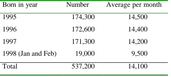
Table 2.Number of observed births per year and monthly average.

Born in year Number Average per month

1995 174,300 14,500

1996 172,600 14,400

1997 171,300 14,200

1998 (Jan and Feb) 19,000 9,500

Total 537,200 14,100

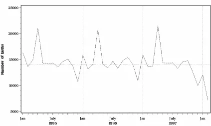
Table 2 and Figure 2 show some aggregates of births and the distribution of births. Except

for the truncation effect clearly visible from November 1997 in Figure 2, the curve is

astonishingly regular over time. Note that this curve represents the row sums of Table 1

apart from partially truncated cells. Note also that the scales of Figures 1 and 2 are very

different: there is far more variability in counts between lags, especially short lags, than

between birth months.

The longest birth lag we can fully observe is 37 months. Longer lags are entirely negligible

as only 15 out of the 16,000 businesses that were born in January 1995 have 37 months birth

lag; only 48 out of 30,000 businesses born in either January or February 1995 have 36

Figure 2. Number of observed births per birth month.

Figure 3. Percent of observed births per day of the month.

Figure 3 displays number of births by day for births in 1995 – 1997. The two panels contrast

businesses started trading on the first of the month, in other months the proportion was even

higher. The eye-catching peak at April 6 in Figure 3 is due to this day being the start of the

taxation year in the UK. In practice, owing to differing interpretation of what constitutes the

start of a business, it is frequently hard to fix on one day as the actual birthday for a

business. The first of the month is often perceived as a convenient date for administrative

purposes, both for the business managers and for the administrative bodies. Also, there is

some heaping visible in Figure 3 in that most of the bars for dates like 10, 15 and so forth

are slightly taller than most other bars. Therefore, month seems to be the smallest viable unit

in the classification of number of births; it does not seem meaningful to split months into

smaller units.

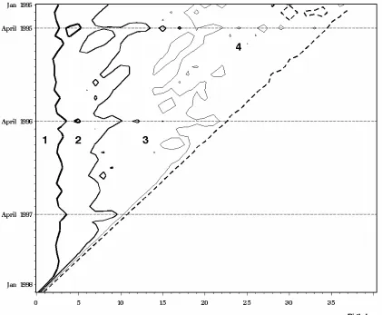
Figure 4 gives a contour plot of Table 1 with partly truncated cells excluded. The area with

the largest counts is to the far left, and then the counts fall as we proceed to the right. The

contour levels are 1096, 148, 21, and 3 (equal distances on a log scale), so area 1 consists of

cells with counts greater than or equal to 1096. A couple of the ‘islands’ in area 4 are counts

smaller than 3. The scarcity of islands in all areas indicates a large degree of homogeneity.

The dashed horizontal lines mark Aprils. Areas 2 and 3, in particular, jut out along the

dotted lines indicating areas with relatively large counts that are stretched to the right. This

is partly due to the fact that there are more births in the month of April, partly due to a more

skewed lag distribution for businesses born in April (the average birth lag is 2.5 months for

businesses born in April and 1.6 months for businesses born in other months). There is also

a diagonal pattern emerging in areas 2 and 3 above the horizontal line that indicates April

1996.

The diagonals correspond approximately to frame introduction months; that is, businesses

that came onto the frame in the same month are located along one or two diagonals running

from right to left in the contingency table. It appears likely that what produces these

diagonal ridges visible in Figure 4 is the reporting of births from Inland Revenue. Since this

is done in a roughly quarterly basis, the notifications of new businesses come in sizable

Figure 4. A contour plot of the contingency table, Table 1. Levels for number of frame

introductions.

3. Models

The number of businesses in transition between birth and frame introduction can be viewed

as a stochastic process over time. The process is not stationary since Figure 4 indicates

among other things that birth lags tend to be longer for businesses born in April than for

businesses born in any other time of year.

In this section we fit models to the upper triangle of the contingency Table 1, excluding

partially truncated cells. It is convenient to confine the class of models to generalised linear

models (e.g. McCullagh and Nelder 1989). A generalised linear model has a random

component, which identifies the probability structure of a response variable Y, a link

function which specifies the relationship between the expected value µ of the response and

the systematic component, which in turn defines a linear function of the explanatory

variables. The systematic component can rather easily accommodate the seasonality and the

Another advantage is that generalised linear models are useful even if the parametric

assumption underlying the model is ill- fitting, since the ML estimation of parameters uses

only the link function, choice of covariates and the variance function V

( )

( )

( )

V = and φ is known as the overdispersion parameter (Davison and Hinkley 1997,

Ch. 7). Thus our approach is essentially semi-parametric.

Let r be the number of rows in the table and let mij be the expected number of businesses

that were born in month i, i = 1, 2, …, r, and that were introduced on the frame in month

1 − + =i j

d , that is with a birth lag j, j = 1, … c, where c is the maximum birth lag we can

observe. For convenience, we renumber the index j tostart at 1 rather than at 0.

We have seen that the birth rate is higher in some months, such as Aprils, than in other

months. It seems plausible that a higher (or lower) birth rate for certain months should give

roughly proportionally larger (or smaller) counts of new businesses for all birth lags. Hence

it seems more plausible that birth months, birth lags and other effects that potentially could

be part of the systematic component are multiplicative rather than additive. This leads us to

the following type of log- linear model:

( )

log , ( 1 )

for i = 1, 2, …, r, j = 1, 2, …, c – i + 1, where u is an intercept and u_{( )}ij is a parameter for

cell i and j in the fully observed triangle in Table 1, with total number of rows r and columns

c = r, here r = 38. Hence the link function is the logarithmic function, which conveniently

converts multiplicative effects on the original scale to additive effects on the log scale. The

variance function V

( )

between the variance of the response and the variance function.

One of the most parsimonious models (i.e. with fewest parameters) that we may be

interested in is a log- linear model with just birth lag effects with u_{( )ij} =u_{lag( )j} , where u_{lag( )j}

is a parameter associated with birth lag j only. Considering Figures 1 and 2, the lag effect

should be far more important than a birth month effect. The latter effect may perhaps even

be dropped altogether. Although this may be an oversimplification, the model with a lag

effect only is interesting as a reference model. Under this model all cells in a column have

Another log- linear model arises from the assumption that the expected cell counts are

separable into quasi- independent row effects and column effects with

( )ij ubirthmonth( )i ulag( )j

u = + . See McDonald (1998) for a definition of quasi- independence and

ML estimation for incomplete tables. Since the underlying stochastic process is not

stationary, there is in fact an interaction between birth months and lags, which the

quasi-independence model fails to capture.

A third model is one with a seasonal effect and a lag effect. The underlying assumption is

that some of the rows of the contingency table show a repetitive pattern in that their effects

are the same and do not depend on year. Figure 2 suggests that all Januaries are similar, and

so forth. It seems reasonable to examine a model with twelve ‘season’ parameters, as

opposed to 38 birth month parameters. The model is:

( )

log = + + , ( 2 )

i = 1, 2, …, 38, j = 1, 2, …, 38−i+1, k=i

(

)

When this model is fitted to the fully observed counts in Table 1, the residuals show a clear

diagonal pattern, a pattern that is visible in Table 1 itself. A diagonal effect can be added to

the model to obtain a better fit. Further, an ‘April effect’ can accommodate part of the

observed longer lags for businesses with births in April:

( )

(

)

log mij =u+useasonk +ulag j +udiagd +αjI k = , ( 3 )

with i, j and k defined as for the model in ( 2 ), d =i+ j−1, a is a parameter and I

( )

The models above were fitted to the fully observed upper triangle of Table 1 using ML

estimation. The usual likelihood ratio test statistic (the ‘G2 statistic’) and the Pearson chi-squared test statistic gave very similar results. The estimation of parameters was done with

Proc Genmod in the SAS System® version 8.02 for Windows, see Zelterman (2002). To

ensure that the Genmod procedure gives correct results, it was run on some well-known

datasets with structural zeroes. To check the numerical stability for the very large table

analysed, the order of columns was changed, likewise the order of the rows for the model

( )ij ubirthmonth( )i ulag( )j

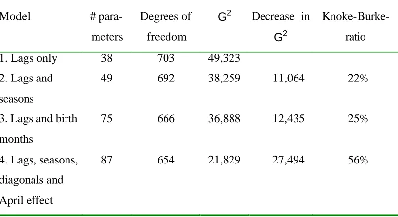
Table 3 gives the values of test statistics for four models. The p- values are not given in the

table below; all are miniscule. The G2- values in Table 3 are extremely large due to the very large cell counts and the large number of cells. It is not meaningful in this application to use

G2-values for significance tests since any useful model would be rejected. We can, however, use G2-values for the comparison of models without formal tests. Another general strategy for dealing with large counts in a contingency table is to look for non-random patterns

among residuals for different models. We will also study how well the models predict future

observations.

Table 3. Goodness of fit for Models 1 – 4.

Model #

para-meters

Degrees of

freedom

G2 Decrease in

G2

Knoke-Burke-ratio

1. Lags only 38 703 49,323

2. Lags and

seasons

49 692 38,259 11,064 22%

3. Lags and birth

months

75 666 36,888 12,435 25%

4. Lags, seasons,

diagonals and

April effect

87 654 21,829 27,494 56%

The Knoke-Burke ratio (Knoke and Burke 1980) is 1−G_alt2 G_ref2 , where G_ref2 is the value of the test statistic under a reference model (here Model 1, lag effect only) and G_alt2 under an alternative model that includes the reference model as a special case. Note that if the

alternative model is the saturated model then the Knoke-Burke ratio attains its maximum,

100%. Knoke and Burke (1980) suggest that this ratio may be used for very large datasets; a

large value indicates that the alternative model is satisfactory. We refer to the models using

the order number in Table 3. Clearly, Model 4 gives the best fit. It is the addition of the

diagonal effect that accounts for the major part of the reduction in G2. Adjusted residuals from Model 4 are large but show no clear pattern.

There are other modelling approaches in the AIDS diagnoses literature. Harris (1990) and

size of the population. Generalised additive models is a class of models that includes

generalised linear models (Hastie and Tibshirani 1986). The link function in these models is

a sum of nonparametric curve components. Davison and Hinkley (1997, examples 7.4 and

7.12) contrast what here is termed Model 3 with a generalised additive model which gives

smoother predictions of unobservable counts in a register of English and Welsh AIDS

patients. In our problem we could take log

( )

( )

( )

Figure 1 suggests that the flat part of the curve may not need a different parameter for each

birth lag, as they have in Models 1 - 4. We leave these ideas for future research.

4. Predicting undercoverage and number of births per month

The models fitted to the upper triangle of the contingency table in Table 1 are now used for

predicting counts in the lower triangle. To fix notation we first give a brief general account

of Poisson log- linear models with ‘matrix notation’. The contingency table has r rows, c

columns and rc=a cells. A general log- linear model is

( )

log , ( 4 )

where m=

(

)

specifies the model. The quantity µ is a parameter and 1 is a vector of ones with the

dimension given by the context. In the presence of structural zeroes the cells in ( 4 ) that

correspond to them would not be included in the model. What remains of m and X after

omission of rows that correspond to structural zeroes is denoted by m* and X*.

For example, consider a two-waytable with r = c = 2 and without structural zeroes. Then a

model with a row factor and a column factor and no interaction would have

            = 1 0 1 0 0 1 1 0 1 0 0 1 0 1 0 1 X .

If the fourth cell is a structural zero

and

( )

log , ( 5 )

with =

(

)

3 * 2 * 1 * , ,

,m m

m K

m .

Let o be the number of cells that are not structural zeroes (o for ‘observed’, a for ‘all’). Let

the set of the fully observed cells be denoted by O and the set of all cells by A. The

difference between A and O is denoted by S, which includes both partially observed cells

and cells with structural zeroes. Like above, we distinguish quantities that are defined for O

only by a star. In general, we have m* =nop*, where

(

)

′ = p1, p2, , po

* _K

p is the vector of

true probabilities under the Poisson distribution and no is the sum of the cell counts in O.

Note that for a model pertaining to O only, *

p is not defined outside O. Thus

(

)

p* =exp * + o

n . ( 6 )

Since the elements of p* add up to unity, we obtain an estimator of p* by summing over the columns of each side of ( 6 ) and replacing the parameter vector ß with, e.g., maximum

likelihood estimates:

( )

[

( )

]

pˆ* =exp *ˆ ′exp *ˆ

. ( 7 )

The estimator µ is

( )

[

( )

]

log

ˆ = − ′ *

o

n

µ . ( 8 )

Let T =To +Ts, where To and Ts are the sum of observable and unobservable cell counts,

respectively. Then it is natural to predict T by Tˆ =T_o +Tˆ_s, where Tˆ_s is a predictor for Ts.

Under the natural assumption that ( 5 ) can for Models 1-3 be extended to model ( 4 ) by

replacing X* with X we have for cell i

(

)

= X_iß

i

m exp , ( 9 )

where and X′i is the ith row of X. Thus X′i corresponds to the ith cell in the contingency

table. The parameters β and µ, which in ( 5 ) are defined for O only, will for Models 1-3

remain the same for A, with the predicted sum over the cells in S

=

s

Tˆ

∑

∑

(

)

∈

∈S = i S ′i +

i mi µˆ

ˆ exp

For Model 4 it is assumed that the diagonal pattern observed for the last 12 months can be

extrapolated periodically; that is, to predict cells along a diagonal d′ in the part of the lower-right triangle where c+1≤d′<c+12, the parameter associated with diagonal

12

− ′

d in the upper- left triangle is used. To predict cells along a diagonal in the next band

of twelve consecutive diagonals, c+13≤d′′<c+24, the parameter associated with diagonal d′′−24 is used, and so on. Thus, only the rightmost band of 12 diagonals in the observed triangle is used for prediction. While this may seem to underutilize the

information, there does not seem to exist a periodic model for the diagonal effects that uses

all observed diagonals and gives smaller prediction errors than the model just described that

only uses the last 12 observed diagonals.

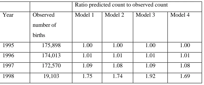
Table 4 gives the number of births aggregated to year levels. As seen in the table the

observed count in 1997 is about 8-9% less than the predicted count. The difference between

the sum of the predicted counts under Model 4 and the observed count is 570,000 – 542,000

= 28,000. Hence, in terms of number of businesses the undercoverage due to reporting

delays is about 1.6% (28,000 on 1.8 million).

Table 4. Observed number of births per year and the predicted to observed ratio.

Ratio predicted count to observed count

Year Observed

number of

births

Model 1 Model 2 Model 3 Model 4

1995 175,898 1.00 1.00 1.00 1.00

1996 174,013 1.01 1.01 1.01 1.01

1997 172,570 1.09 1.08 1.09 1.08

1998 19,103 1.75 1.74 1.92 1.69

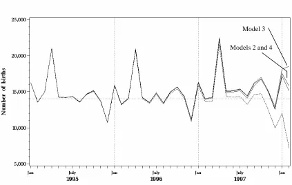
Figure 5 shows the observed and predicted number of births per month for Models 2 - 4.

The dashed curve in Figure 5 is the same one as in Figure 2. Judging from Figure 5 there is

little to choose between the prediction methods with only Model 3 being somewhat

separated from the others. There is a 1% truncation effect as early as September 1995 that

Figure 5. Predicted number of births per month under Models 2-4. The observed

counts are graphed with a dashed line.

5. Prediction error

To assess the prediction error, we can turn the clock back, for example to the end of May

1995, and pretend that all observed businesses born afterwards are unknown. Hence there

will be a 5x5 square subtable with observed counts in the upper- left triangle and ‘missing’

counts in the lower-right triangle. A natural estimate of the error is obtained by estimating

parameters for the upper triangular subtable and basing the prediction error on the difference

between the observed and predicted counts in the lower-right triangle.

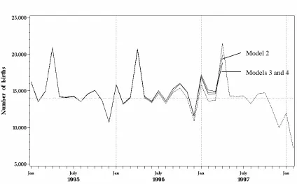
Using this approach, Figure 6 shows the number of births per month for data cut off at the

end of April 1997. The dashed curve is the number of births per month obtained from the

full original table (that is, it is the same curve as in Figure 2). Models 3 and 4 are

indistinguishable while Model 2 predicts the rise in births in April rather better than the

other models.

Thus the ends of the solid curves in Figure 6 show the predicted number of births for the

month that corresponds to the last row of the particular triangular subtable which has been

obtained by cutting the full table off at the end of April 1997.

Model 3

Figure 6. Predicted number of births based on data up to 30 April 1997: Models 2 - 4

and observed counts as at 28 February 1998 (dashed line).

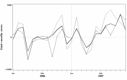
Figures 7 and 8 show the prediction errors for a series of subtables, from the one obtained by

cutting off at the end of December 1995 to the one where data after December 1997 were

discarded. In Figure 7 the final- month errors are shown, defined as the difference between

the predicted number of births in the last month of the subtable and the observed number of

births in the same month in the part of the original table covered by the subtable.

The part of Figure 7 to the right of July 1997 is clearly influenced by the bias resulting from

truncation of the original series. In the beginning of the series the error is, as expected, large

due to the fact that in the beginning of the series there is less data for the estimation of

parameters. It seems reasonable to forego the prediction errors before July 1996 and after

July 1997.

As seen in Figure 7, Model 2 gives smaller final- month errors than Model 3 for each month

in this interval. This may seem paradoxical since Model 3 has more parameters and gave a

better fit to the upper triangle of the contingency table (see Table 3). However, the models

play two roles here. One is to fit counts in the upper triangle of the contingency table. The

other is to be a tool for prediction. Good performance in one of these roles does not

necessarily imply good performance in the other. Model 3 does not draw on the seasonal

Model 2

pattern. Stated somewhat loosely, Model 2 borrows strength from similar months in

previous years. With Model 3, the predictions depend completely on single rows of the table

and are much more variable. Model 2 has the additional advantage over model 3 that it

allows prediction beyond February 1998. Model 4 often gives smaller errors than Model 2,

but certainly not always.

Figure 7. Difference between predicted and observed number of births for the final

month in successive subtables. Three models: Model 2 (thick line ), Model 3 (dashed

line ), and Model 4 (thin line ).

The largest prediction error in absolute terms for Model 2 in the interval July 1996 – July

1997 is about 1800, which occurs in November 1996. Thus the ratio of the prediction error

to the average number of births per month, 14,000, is about 17%. Cross-validating in the

same way for the second last row gives 2000 as the estimated prediction error. The

estimated error for the third last row is 1700. The sum of all rows is about 10,000. Thus, a

conservative estimate of the error of the estimated undercoverage is 10,000.

The difference between the sum of monthly predictions and observations is a measure of

error more directly connected to the estimation of the undercount. These differences for a

sequence of subtables are displayed in Figure 8. In the beginning of the series the difference

is negative because the predictions for 1995 are too low. The difference becomes positive

Figure 8 makes it clear that Model 4 is better than Model 2. As seen in Figure 8, the largest

prediction error in absolute terms for Model 2 in the interval July 1996 – July 1997 is less

than 10,000. For Model 4 the largest error is less than 6,000.

Figure 8. Difference (in thousands) between the sum of predicted number of births and

observed number of births in successive subtables. Three models: Model 2 (thick line ),

Model 3 (dashed line ), and Model 4 (thin line ).

6. Bias resulting from reporting delays

The undercoverage will lead to a negative bias in an estimate of the total or mean. Suppose

the aim is to estimate the total =

∑

U k

y y

t of a study variable y′=

(

)

{

}

month i and reporting delay j. The total of the unseen part of the population, tUs, is the sum

of =

∑

Uij k yij y

t over the not fully observed cells (i, j) in Table 1, each of which holds the

population Uij.

We draw on actuarial science to find a method for predicting tUs, which is in that context

interpreted as, for example, the sum of incurred but not reported (IBNR) losses for which

the clients are insured. The chain ladder method is widely used in insurance practice. For

and let

∑

= j xi ij t C

1

ι ι

be the cumulative totals of the auxiliary variable for businesses with

birth month i and birth lag not longer than j. Introduce the development factors

1 1 1 1 , 1 1 ˆ − + − = − + − =        

=

∑

∑

j C C

λ ,

where j≤r and r = c is the total number of rows (columns) in the table. The development factors are applied to the largest observed cumulative total in row i, that is Ci,r-i+1 to give an

estimate of the cumulative total for the subsequent columns in row i:

2 1 , 2 , ˆ ˆ + − + − +

−i = ir i r i r

i C

C λ ,

3 2 1 , 3

, ˆ ˆ

ˆ + − + − + − +

−i = ir i r i r i r

i C

C λ λ ,

and so on. Hence the assumption, for simplicity expressed here for unobservable cell (2,c)

only, is that

c c c c C C C C 2 1 1 , 2 1 , 1 ₌ − − .

Mack (1991) and Renshaw and Verrall (1998) show that the chain ladder technique

necessarily gives the same cell predictions as the quasi- independence model, which is

labelled Model 3 in this chapter. An extension of the chain ladder technique is thus to apply

Models 2 and 4 to observed totals of some frame variable to predict non-observed cell totals

of this variable.

There are other approaches in actuarial science. In the often used Bornhuetter-Ferguson

technique (Bornhuetter-Ferguson 1972), the Cic are taken as known constants as though they

were available in external sources and the only free parameters are the lag parameters. Using

an argument from credibility theory, Mack (2000) discusses the approach where the final

predictions are linear combinations of the Bornhuetter-Ferguson predicted values and the

predictions obtained through the chain- ladder method. Overviews of the IBNR prediction

problem are given by England and Verrall (2002) and De Vylder (1996, Ch. 7). It is usual to

assume stationarity for IBNR prediction.

Alternatively, one can fit a model to the frame variable to obtain an estimate of the expected

value in each cell and multiply this by the predicted number of units in that cell. Klugman,

separately has some advantages in the IBNR losses context. In the situation in this paper, it

is useful to compare the distribution of the study variable for different birth lags with that of

the counts. Also, to investigate the impact of legal and procedural changes (for exa mple if

the VAT threshold for mandatory reporting to the relevant UK authority changes or if new

proving processes are introduced at the ONS) it is helpful to model the distribution of the

counts and the study variable separately to avoid confounding. We do not pursue this

approach here.

Figure 9. Average turnover in £000 at frame introduction against birth lag.

The variable turnover at frame introduction was stored for the businesses whose counts are

reported in Table 1. Figure 9 shows that businesses that are very large when they come onto

the frame tend to have long birth lags. It is believed that few of these large businesses are

genuinely new; rather they are the result of mergers and other types of restructuring. To

avoid duplication large businesses that are reported as new are subjected to an often lengthy

proving process which can not usually be done without the help of the business itself.

However, there is little information stored on the frame on the history of a business.

Figures 10 and 11 show the distribution of total turnover at frame introduction against birth

lag and birth month. The similarity of these to Figures 1 and 4 suggests that the cell totals of

Figure 10. Total turnover at frame introduction in £bn against birth lag (months).

Figure 11. A contour plot of levels for total turnover at frame introduction. The levels

Figure 12. Difference in £bn between predicted and observed number of births for the

final month in successive subtables. Three models: Model 2 (thick line), Model 3

(dashed line), and Model 4 (thin line).

Cross-validation errors that parallel those of Figure 7 are displayed in Figure 12. The

estimated total undercoverage is £2.400bn. Unfortunately, the errors displayed in Figure 12

are of similar size as the point estimate. The large businesses with long lags, clearly visible

in the contour plot but also in Figure 10, make prediction intrinsically difficult. They enter

the frame irregularly and produce large variation in total turnover per birth month.

7. Discussion

Undercoverage is arguably the most important type of frame imperfection. We believe that

the work initiated here provides a useful measure of frame quality. A time series of the

undercoverage as estimated each month in terms of number of businesses is a useful tool for

monitoring frame quality. For example, a long-term increase will spur questions about what

developments in the processes cause the changes in the reporting delay distribution.

We have predicted gross totals with a log-linear model. The prediction error was estimated

1998 the undercount was 28,000 businesses, or 1.6% of all registered businesses. The error

of this estimate was predicted to be less than 6,000.

The sum of the turnover of the unobservable businesses was not possible to predict with any

accuracy due to a heavy tail in the reporting delay distribution. The heavy tail is due to the

fact that many businesses that are very large when they enter the frame are not genuinely

new businesses. Since the history of businesses is currently not stored on the business

register of the ONS, it has been proposed to create a new life status variable that will store

more complete information about changes to businesses. This will be a log of events that

have occurred in the life of the business and will allow the separation of genuinely new

businesses from businesses that are new only in a legal sense. Being able to predict

accurately the bias of a frame variable enables estimation of the bias of survey variables

through models of the association between the frame variable and each survey variable.

8. References

Agresti, A. (1990). Categorical Data Analysis. New York: Wiley.

Bornhuetter, R.L. and Ferguson, R.E. (1972). The Actuary and IBNR. Proceedings of the

Casualty Actuarial Society, LIX, 181-195.

Davison, A.C. and Hinkley, D.V. (1997). Bootstrap Methods and their Application.

Cambridge University Press.

De Vylder, F.E. (1996). Advanced Risk Theory. Brussels: Editions de l'Universite de

Bruxelles.

England, P.D. and Verrall, R.J. (2002). Stochastic Claims Reserving in General Insurance.

Paper presented to the Institute of Actuaries, London, UK, 28 Jan 2002.

Haberman, S. and Renshaw, A.E. (1996). Generalized Linear Models and Actuarial Science.

The Statistician, 45, 407-436.

Harris, J.E. (1990). Reporting Delays and the Incidence of AIDS. Journal of the American

Statistical Association, 85, 915-924.

Hastie, T. and Tibshirani, R. (1986). Generalized Additive Models. Statistical Science, 1,

297-310.

Klugman, S.A., Panjer, H.H., and Willmot, G.E. (1998). Loss Models: From Data to

Knoke, D. and Burke, P (1980). Log-Linear Models. Sage University Paper Series on

Quantitative Applications in the Social Sciences (07-020). Beverly Hills and London:

Sage Publications.

Mack, T. (1991). A Simple Parametric Model for Rating Automobile Insurance or

Estimating IBNR Claims Reserves. ASTIN Bulletin, 21, 9-109.

Mack, T. (2000). Credible Claims Reserves: The Benktander Method. ASTIN Bulletin, 30,

333-347.

McCullagh, P. and Nelder, J.A. (1989). Generalized Linear Models, 2nd ed. London:

Chapman & Hall.

McDonald, J.W. (1998). Quasi- Independence. In Encyclopedia of Biostatistics, eds. P.

Armitage and T. Colton. New York: Wiley, 3637-3639.

Renshaw, A.E. and Verrall, R.J. (1998). A Stochastic Model Underlying the Chain- Ladder

Technique. British Actuarial Journal, 4, 903-923.

Sellero, C.S., Fernández, E.V., Manteiga, W.G., Otero, X.L., Hervada, X., Fernández, E.,

and Taboada, X.A. (1996). Reporting Delay: a Review with a Simulation Study and

Application to Spanish AIDS Data. Statistics in Medicine, 15, 305-321.

Wang, M.-C. (1992). The Analysis of Retrospectively Ascertained Data in the Presence of

Reporting Delays. Journal of the American Statistical Association, 87, 397-406.