ISSN Online: 2327-4379 ISSN Print: 2327-4352
DOI: 10.4236/jamp.2018.68138 Aug. 9, 2018 1625 Journal of Applied Mathematics and Physics
Improving Wilson-
θ
and Newmark-
β
Methods
for Quasi-Periodic Solutions of Nonlinear
Dynamical Systems
G. Liu, Z. R. Lv, Y. M. Chen
*Department of Applied Mechanics and Engineering, School of Aeronautics and Astronautics, Sun Yat-sen University, Guangzhou, China
Abstract
Quasi-periodic responses can appear in a wide variety of nonlinear dynamical systems. To the best of our knowledge, it has been a tough job for years to solve quasi-periodic solutions, even by numerical algorithms. Here in this paper, we will present effective and accurate algorithms for quasi-periodic solutions by improving Wilson-θ and Newmark-β methods, respectively. In both the two methods, routinely, the considered equations are re-arranged in the form of incremental equilibrium equations with the coefficient matrixes being updated in each time step. In this study, the two methods are improved via a predictor-corrector algorithm without updating the coefficient matrixes, in which the predicted solution at one time point can be corrected to the true one at the next. Numerical examples show that, both the improved Wilson-θ
and Newmark-β methods can provide much more accurate quasi-periodic solutions with a smaller amount of computational resources. With a simple way to adjust the convergence of the iterations, the improved methods can even solve some quasi-periodic systems effectively, for which the original methods cease to be valid.
Keywords
Wilson-θ Method, Newmark-β Method, Quasi-Periodic Solution, Predictor-Corrector Algorithm
1. Introduction
Both Wilson-θ and Newmark-β methods are generally used approaches for solving numerical solutions of dynamical systems [1]-[6]. As we know, a funda-mental assumption of the Wilson-θ method lies in that, the acceleration changes
How to cite this paper: Liu, G., Lv, Z.R. and Chen, Y.M. (2018) Improving Wil-son-θ and Newmark-β Methods for Qua-si-Periodic Solutions of Nonlinear Dynam-ical Systems. Journal of Applied Mathe-matics and Physics, 6, 1625-1635. https://doi.org/10.4236/jamp.2018.68138
DOI: 10.4236/***.2018.***** 1626 Journal of Applied Mathematics and Physics linearly in a single time step [7]. For this reason, the Wilson-θ is considered to be one of linear acceleration methods. One of the best merits of this method is that its result is unconditionally stable when the internal parameter θ is chosen to be larger than 1.37 [8]. The Newmark-β method is in essence an extension of linear acceleration method [9]. When solving linear problems, both the two me-thods can provide accurate results by adjusting the internal parameters.
For some nonlinear problems, sometimes the two methods would provide false results, especially when there are quasi-periodic or chaotic responses [10]. Even worse, the methods may even cease to be valid for some cases, for instance leading to numerical divergence as shown later. Fu et al. [11] proposed an ap-proximate method to linearize a quasi-periodic nonlinear equation, and suggested a gradual integration process based on the Wilson-θ method. To the best of our knowledge, it is tough to make such a linearization to complex quasi-periodic sys-tems especially when strongly nonlinearities are taken into account. Even though the linearization is done successfully, it will pose restriction to the computational accuracy [12] [13].
In this paper, both the Wilson-θ and Newmark-β methods will be improved with the help of a predictor-corrector algorithm. This algorithm is based on the incremental process which makes Wilson-θ and Newmark-β methods free of repeated linearizations of the nonlinear terms. The initial solution is predicted at the previous time point and corrected recursively to be the true one at the next point. Numerical solutions have been successfully obtained for quasi-periodic responses of both autonomous and non-autonomous nonlinear dynamical sys-tems. Interestingly, the results show that the iterative correction of the predicted solution can converge within two iterations, which ensures the improved thods with high computational efficiency. Most importantly, the improved me-thods can directly deal with a variety of quasi-periodic dynamical systems with even strong nonlinearities, as there is no requirement of linearizing the consi-dered equations.
2. Classical Wilson-
θ
and Newmark-
β
Methods
2.1. Linearization
The nonlinear dynamical system is expressed as the following form
( ) ( ) ( )
, ,( )
P x t x t x t =Q t (1) where x t x t x t
( ) ( ) ( )
, , represent the generalized acceleration, velocity and dis-placement, respectively. After a step length ∆t, the following equation will be obtained as(
) (
,) (
,)
(
)
DOI: 10.4236/***.2018.***** 1627 Journal of Applied Mathematics and Physics
(
, ,)
(
, ,)
(
, ,)
(
)
( )
t t t
P x x x P x x x P x x x
x x x Q t t Q t
x x x
∂ ∂ ∂ ∆ + ∆ + ∆ = + ∆ − ∂ ∂ ∂ (3)
which can be expressed in matrix form as
M x C x K x∆ + ∆ + ∆ = ∆ Q (4) with coefficient matrixes as
(
, ,)
(
, ,)
(
, ,)
(
)
( )
, , ,
t t t
P x x x P x x x P x x x
M C K P Q t t Q t
x x x
∂ ∂ ∂ = = = ∆ = + ∆ − ∂ ∂ ∂
At the beginning of each time step, one should calculate the coefficient ma-trixes. One possible way is to substitute into Equation (4) the velocity, accelera-tion and displacement of the previous time step, i.e., x x t x t ,
( ) ( )
, . It is worth noting that, however, this treatment will bring serious numerical errors as the higher-order terms are all removed from the Taylor expansion. On the other hand, Equation (1) will be unbalanced if we substitute(
) (
,) (
,)
x t+ ∆t x t+ ∆t x t+ ∆t
into the coefficient matrixes. Denote the unba-lanced term as
(
) (
,) (
,)
(
)
R P x t= + ∆t x t + ∆t x t+ ∆t −Q t+ ∆t
(5) where R is also the truncation error for each calculation. The precision of the computing result can be controlled by adjusting R to a relatively low magnitude [14].
2.2. Solving Incremental Equation
A basic assumption of the Wilson-θ method is that the acceleration varies li-nearly between time
[
t t, + ∆θ t]
, so that the velocity and displacement can be expressed as(
) ( )
(
) ( )
(
) ( )
( ) ( )
2(
)
( )
22 6
t
x t t x t x t t x t
t
x t t x t tx t x t t x t
θ θ θ θ ∆ + ∆ = + + ∆ + ∆ + ∆ = + ∆ + + ∆ + (6)
Rewrite Equation (6) equivalently in the incremental form and substitute it into (4), we can deduce the incremental displacement equation at
[
t t, + ∆θ t]
K x∆ θt = ∆Q (7)
in which
( )
( )
( )
( )
( )
2
3 6 ,
6
3 3
2
K K C M
t t
t
Q Q x t x t C x t x t M
t θ θ θ θ = + + ∆ ∆ ∆ ∆ = ∆ + + + + ∆
(8)
DOI: 10.4236/***.2018.***** 1628 Journal of Applied Mathematics and Physics
0 1 2
3 4 5
6 7 8
t
t
t
x a x a x a x
x a x a x a x
x a x a x a x
θ θ θ ∆ = ∆ + + ∆ = ∆ + + ∆ = ∆ + + (9)
where the coefficients a ii, =0,1, ,8 are all listed in Appendix. And, the sys-tem response at time t+ ∆t could be finally obtained as
(
)
( )
(
)
( )
(
)
( )
x t t x t x
x t t x t x
x t t x t x
+ ∆ = + ∆ + ∆ = + ∆ + ∆ = + ∆ (10)
Similar to Equation (6), when the Newmark-β method is employed we can obtain
(
)
(
) ( )
( )
( )
(
) ( ) (
) ( )
(
)
2
1 1 1 1
2 1
x t t x t t x t x t x t
t t
x t t x t tx t tx t t
α α α δ δ + ∆ = + ∆ − − + − ∆ ∆ + ∆ = + − ∆ + ∆ + ∆ (11)
with α and δ are priorly given parameters. Also, rewrite Equation (11) in the incremental form and substitute it into (4), then we can obtain
0 1 2
3 4 5
x b x b x b x x b x b x b x ∆ = ∆ + + ∆ = ∆ + +
(12)
with the expressions of b ii, =0,1, ,5 in Appendix. Substituting Equation (12) into (10) yields the response at time t+ ∆t.
3. Improving Wilson-
θ
and Newmark-
β
Methods
To elucidate the improved methods, we consider the following dynamic equa-tion
( )
( )
( ) ( )
(
, ,)
Mx t +Cx t +K x x t =F x x t (13)
If Equation (13) is linear such that F x x t
(
, ,)
is independent upon either dis-placement x or velocity x, the Wilson-θ method can also be straightforwardly implemented by carrying out the following proceduresStep 1a: Given any initial conditions (x x 0, 0 and x0), time step ∆t as well as θ≥1.37, calculate the integral constants c0~c8 shown in Appendix.
Step 2a: Compute the payload, Ft+ ∆θt, at time t+ ∆t
(
)
(
)
(
1 3)
0 22 2
t t t t t t t t t
t t t
F F F F M c x c x x
C c x x c x
θ θ
+ ∆ = + +∆ − + + +
+ + +
(14)
Step 3a: Solve the displacement at time t+ ∆θ t according to the following
equation
*
t t t t
K x+ ∆θ =F+ ∆θ
(15) where *
0 1
K =K c M c C+ + .
Step 4a: Finally, calculate the displacement, velocity and acceleration at time
DOI: 10.4236/***.2018.***** 1629 Journal of Applied Mathematics and Physics
(
)
(
) ( )
( )
( )
(
) ( )
(
) ( )
(
) ( )
( )
(
)
( )
4 5 6
7
8 2
x t t c x t t x t c x t c x t
x t t x t c x t t x t
x t t x t tx t c x t t x t
θ
+ ∆ = + ∆ − + +
+ ∆ = + + ∆ +
+ ∆ = + ∆ + + ∆ +
(16)
Then go to Step 1a to calculate the responses at the next time step.
Also, the Newmark-β method is capable of solving Equation (13) as long as it is linear, by employing the following procedures
Step 1b: Given any initial conditions (x x 0, 0 and x0), time step ∆t as well as δ≥0.50,
α
≥0.25 0.5(
+δ
)
2, compute the constants d0~d7 as shown in Appendix.Step 2b: Compute the payload, Ft+ ∆θt, at time t+ ∆t
(
0 2 3)
(
1 4 5)
t t t t t t t t t t
F+∆ =F+∆ +M d x d x d x+ + +C d x d x d x+ + (17) Step 3b: Solve the displacement at time t+ ∆t according to the following equation
*
t t t t
K x+∆ =F+∆ (18)
where *
0 1
K =K d M d C+ + .
Step 4b: Finally, calculate the displacement, velocity and acceleration at time
t+ ∆t according to the rules
(
)
(
) ( )
( )
( )
(
) ( )
( )
(
)
(
)
0 2 3
6 7
* / t t
x t t d x t t x t d x t d x t
x t t x t d x t d x t t
x t t F+∆ K
+ ∆ = + ∆ − − −
+ ∆ = + ⋅ + ⋅ + ∆
+ ∆ =
(19)
Then go to Step 1b to calculate the responses at the next time step.
Note that, the above two methods are designed to solve linear systems. For nonlinear systems such as a cubic stiffness being included [15], the payload cannot be directly determined using either Step 2a or Step 2b, because the term
t t
F+∆ in both Equations (14) and (17) is a function of the responses (i.e.,
, , t t t t t t x+∆ x+∆ x+∆
), which are to be determined at the next time step. For this rea-son, Fu et al. [11] suggested an approximate method by transforming the nonli-near problem into linonli-near one during one time step. As will be shown in the nu-merical examples, this method requires a large amount of computational re-sources. Even worse, it ceases to be valid in some cases possibly because of large errors accumulation in the procedure of linearization.
The key procedure of the improved methods is to calculate the responses by a predictor-corrector algorithm, without transforming the nonlinearities into li-near ones.
Denote the state responses of the system at time t as
{ }
u t ={
x t x t x t( ) ( ) ( )
, ,}
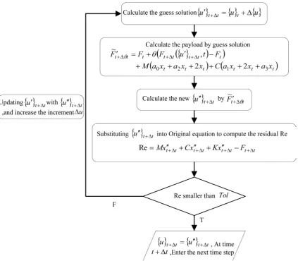
(20) After the time ∆t, the state responses are rewritten asDOI: 10.4236/***.2018.***** 1630 Journal of Applied Mathematics and Physics second steps (Step 2a and Step 2b) which aim at calculating the payload are re-placed by the following predictor-corrector algorithm
Step A: Predict the solution
{ }
u′ t+∆t at t+ ∆t according to priorly givenresponses
{ }
u t with a small increment ∆u.Step B: Compute the payload Ft+ ∆′θt by applying the predicted solution
{ }
u′ t+∆t to Equation (14) or (17).Step C: Obtain a new solution
{ }
u′′ t+∆t at t+ ∆t by applying Ft+ ∆′θt to Eqs.(15-16) or (18-19);
Step D: Correct
{ }
u′′ t+∆t by proceeding Steps B-C-D if necessary, until theresidual Re |=Mx t
( )
+Cx t( )
+K x x t( ) ( )
−F x x t(
, , |)
is smaller than a given tolerance Tol.For more details, Step 2a and Step 2b will be realized by the procedures dis-played in Figure 1.
In real practice, there are two key variables to be elaborately chosen such as the initial increment ∆u and the tolerance Tol. In principle, a small value of
u
[image:6.595.117.541.319.689.2]∆ is helpful to the convergence of the predictor-corrector algorithm. In our
DOI: 10.4236/***.2018.***** 1631 Journal of Applied Mathematics and Physics numerical study, ∆u is chosen randomly chosen to be at the order of 10-6. Differently, the value of Tol should be chosen to be relatively large to guaran-tee the convergence. In this paper, Tol is chosen as Tol O t= (∆2) because
both the Wilson-θ and Newmark-β methods generally have a precision of the second order.
4. Numerical Examples
In this section, a nonlinear dynamical system will be presented as numerical examples to validate the presented methods for solving quasi-periodic solutions.
It should be pointed out that, both the classical Wilson-θ and Newmark-β
methods are incapable of solving nonlinear dynamical systems. As mentioned above, Fu et al. [11] suggested an approximate approach to enable Wilson-θ be capable of doing a nonlinear problem. The Wilson-θ modified by Fu et al. [11] will also be employed in all the following numerical studies, for the purpose of comparing the effectiveness and precision of the presented improved methods.
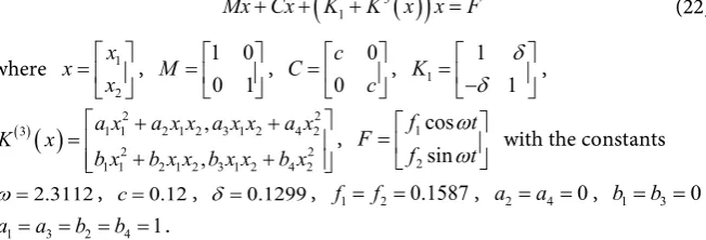
Considering the forced system is subjected to external excitations varying over time domain such as [16]
( )
(
3)
1
Mx Cx K K x x F+ + + =
(22)
where 1
2 x x x = ,
1 0 0 1 M =
, 0 0 c C c = , 1
1 1 K = δ δ
−
,
( )3
( )
1 12 2 1 2 3 1 2 4 222 2
1 1 2 1 2 3 1 2 4 2
, ,
a x a x x a x x a x
K x
b x b x x b x x b x
+ + = + + , 1 2 cos sin f t F f t ω ω =
with the constants 2.3112
ω= , c=0.12, δ =0.1299, f1= f2=0.1587, a2=a4=0, b b1= 3=0, 1 3 2 4 1
a a b b= = = = .
Also, the time step is chosen as ∆ =t 0.01 in this example. Figure 2 shows the comparisons of the displacement obtained by RK and the Wilson-θ methods, respectively. There is a slight discrepancy even at the early stage of the solution domain. As t increases further, the errors accumulate gradually resulting into noticeable differences. For quasi-periodic solutions, the coefficient matrix of the incremental balance equation should be corrected at every iteration step during calculation [17], which is possibly responsible for the rapid growing errors. The quasi-periodic solutions obtained by the improved methods are shown in Figure 3, also compared with the RK results. Nice agreement between the obtained sol-tuions domenstrate that both the improved Wilson-θ and Newmark-β methods can provide much more accurate quasi-periodic solutions.
To further check the computaion accuracy, the error curves provided by the obtained results are shown in Figure 4. The error of the classical Wilson-θ is nearly of the same magnitue of the quasi-periodic responses, whereas the errors of the improved methods are at a much lower level.
[image:7.595.210.536.338.449.2]DOI: 10.4236/***.2018.***** 1632 Journal of Applied Mathematics and Physics Figure 2. Displacement of Equation (23) obtained by RK and classical Wilson-θ methods [11], respectively.
Figure 3. Displacement of Equation (23) obtained by RK, improved Wilson-θ and im-proved Newmark-β methods, respectively.
[image:8.595.209.537.373.622.2]DOI: 10.4236/***.2018.***** 1633 Journal of Applied Mathematics and Physics Figure 4. Error curves of the obtained results for Equation (23) with RK results as the references.
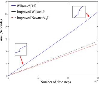
Figure 5. CPU running time versus the number of time steps for the classical Wilson-θ, improved Wilson-θ and improved Newmark-β methods, respectively.
5. Conclusions
Two improved methods have been proposed based on Wilson-θ and Newmark-β
[image:9.595.208.539.351.636.2]dynam-DOI: 10.4236/***.2018.***** 1634 Journal of Applied Mathematics and Physics ical systems. In order to avoid the same linearization procedure of Wilson-θ and Newmark-β methods, an improved fast algorithm is proposed in this paper, which enables both the two methods be capable of solving the quasi-periodic responses of nonlinear dynamical systems. In this algorithm, the solution at the next time step is first predicted according to the known one at the present time. And the predicted solution is corrected by iterative manner, which together pro-vides us with a predictor-corrector algorithm.
Numerical examples have showed that, compared with the classical method, the improved methods can provide much more accurate quasi-periodic res-ponses with less computational resources. Moreover, the improved methods are sometimes valid for systems for which the classical method is not. In addition, the convergence criterion is simple and effective for the presented methods, which guarantees both the computation accuracy and efficiency.
Acknowledgements
This work is supported by the National Natural Science Foundation of China (11572356, 11672337).
Conflicts of Interest
The authors declare no conflicts of interest regarding the publication of this paper.
References
[1] Fang, D.P. and Wang, Q.F. (2010) Accuracy Analysis of Wilson-θ Method with Modified Acceleration. J. Vib. Shock, 29, 216-218.
[2] Dai, H.L., Dai, T. and Yan, X. (2015) Thermoelastic Analysis for Rotating Circular HSLA Steel Plates with Variable Thickness. Appl. Math. Comput., 268, 1095-1109. https://doi.org/10.1016/j.amc.2015.07.017
[3] Zupan, E., Saje, M. and Zupan, D. (2013) Dynamics of Spatial Beams in Quaternion Description Based on the Newmark Integration Scheme. Comput. Mech., 51, 47-64. https://doi.org/10.1007/s00466-012-0703-0
[4] Dabaghi, F., Petrov, A., Pousin, J., et al. (2016) A Robust Finite Element Redistribu-tion Approach for Elastodynamic Contact Problems. Appl. Numer. Math., 103, 48-71. https://doi.org/10.1016/j.apnum.2015.12.004
[5] Krause, R. and Walloth, M. (2012) Presentation and Comparison of Selected Algo-rithms for Dynamic Contact Based on the Newmark Scheme. Appl. Numer. Math., 62, 1393-1410. https://doi.org/10.1016/j.apnum.2012.06.014
[6] An, C. and Su, J. (2011) Dynamic Response of Clamped Axially Moving Beams: Integral Transform Solution. Appl. Math. Comput., 218, 249-259.
https://doi.org/10.1016/j.amc.2011.05.035
[7] Wilson, E.A. and Parsons, B. (1970) Finite Element Analysis of Elastic Contact Problems Using Differential Displacements. Int. J. Numer. Method Eng., 2, 387-395. https://doi.org/10.1002/nme.1620020307
[8] Liu, J.B. and Du, X.L. (2005) Structural Dynamics. China Machine Press, Beijing. [9] Cho, I.H. and Porter, K. (2015) Three-Stage Multiscale Nonlinear Dynamic Analysis
DOI: 10.4236/***.2018.***** 1635 Journal of Applied Mathematics and Physics [10]Janin, O. and Lamarque, C.H. (2001) Comparison of Several Numerical Methods for
Mechanical Systems with Impacts. Int. J. Numer. Method Eng., 51, 1101-1132. https://doi.org/10.1002/nme.206
[11]Fu, Z.G. and Ren, F.C. (2001) A Linearization and an Integral Method Step by Step for the General Strong Non-Linear Vibration Differential Equation. J. Nonlinear Dyn. Sci. Tech., 8, 359-364.
[12]Mirzaee, A., Shayanfar, M. and Abbasnia, R. (2014) Damage Detection of Bridges Using Vibration Data by Adjoint Variable Method. Shock Vib., 2014, 1-17. https://doi.org/10.1155/2014/698658
[13]Grammont, L., Vasconcelos, P.B. and Ahues, M. (2016) A Modified Iterated Projec-tion Method Adapted to a Nonlinear Integral EquaProjec-tion. Appl. Math. Comput., 276, 432-441. https://doi.org/10.1016/j.amc.2015.12.019
[14]Ferziger, J.H. and Peric, M. (2012) Computational Methods for Fluid Dynamics. Springer Science & Business Media.
[15]Chen, Y.M., Liu, Q.X. and Liu, J.K. (2014) Limit Cycle Analysis of Nonsmooth Aeroelastic System of an Airfoil by Extended Variational Iteration Method, Acta Mech, 225, 1-9. https://doi.org/10.1007/s00707-013-1026-8
[16]Kirrou, I. and Belhaq, M. (2016) On the Quasi-Periodic Response in the Delayed Forced Duffing Oscillator, Nonlinear Dyn, 84, 2069-2078.
https://doi.org/10.1007/s11071-016-2629-0
[17] Ren, F.C. (1997) Research on the Shafting Bending Torsional Coupling Vibration in Big Turbogenerator Unit. Ph.D. Dissertation, North China Electric Power University.
Appendix
Coefficients for Wilson-θ method based on the incremental equation
0 3 2
6 a
t θ =
∆ , 1 2
6 a
t θ = −
∆ , a2= −θ3, 3 2 3 a
t θ =
∆ , 4 2
3 a
θ
= − , a5= −1 23
θ
∆t ,
6 3
1 a
θ
= , 7 2
3 1 a t
θ
= − ∆ , 2 8 12 1 1 a = −θ
∆t
Coefficients for Newmark-β method based on the incremental equation
0 2 1 b t α =
∆ , b1= −α1∆t, b2= −21α , b3 t δ α =
∆ , b4 δ α
= − , b5 1 2
δ α = +
Integral constants in classical Wilson-θ method
( )
0 2 6 c t θ =∆ , 1 3 c
t θ =
∆ , c2= ⋅2 c1, 3 2 t
c =∆ ⋅θ, 0
4 c c
θ
= , 2
5 c
c θ
= − , c6= −1 θ3,
7 2t
c =∆ , 8 2
6 t
c =∆
Integral constants in classical Newmark-β method
0 2 1 d t α =
∆ , d1=αδ∆t, d2=α1∆t, d3=21 1α− , d4=δα−1, d5 2t 2
![Figure 2. Displacement of Equation (23) obtained by RK and classical Wilson-θ methods [11], respectively](https://thumb-us.123doks.com/thumbv2/123dok_us/9275054.419523/8.595.209.537.373.622/figure-displacement-equation-obtained-classical-wilson-methods-respectively.webp)