Unsupervised Anomaly Detection in Network Intrusion Detection
Using Clusters
Kingsly Leung
Christopher Leckie
†
†NICTA Victoria Laboratory
Department of Computer Science and Software Engineering The University of Melbourne
Parkville, Victoria 3010 Australia Email:[email protected]
Abstract
Most current network intrusion detection systems em-ploy signature-based methods or data mining-based methods which rely on labelled training data. This training data is typically expensive to produce. More-over, these methods have difficulty in detecting new types of attack. Using unsupervised anomaly detec-tion techniques, however, the system can be trained with unlabelled data and is capable of detecting pre-viously “unseen” attacks. In this paper, we present a new density-based and grid-based clustering algo-rithm that is suitable for unsupervised anomaly de-tection. We evaluated our methods using the 1999 KDD Cup data set. Our evaluation shows that the accuracy of our approach is close to that of existing techniques reported in the literature, and has several advantages in terms of computational complexity. 1 Introduction
With the increased usage of computer networks, se-curity becomes a critical issue. A network intrusion by malicious or unauthorised users can cause severe disruption to networks. Therefore the development of a robust and reliable network intrusion detection system (IDS) is increasingly important.
Traditionally, signature based automatic detection methods have been widely used in intrusion detection systems. When an attack is discovered, the associated traffic pattern is recorded and coded as a signature by human experts, and then used to detect malicious traffic. However, signature based methods suffer from their inability to detect new types of attack. Further-more the database of the signatures is growing as new types of attack are being detected, which may affect the efficiency of the detection.
Other methods have been proposed using machine learning algorithms to train on labelled network data, i.e., with instances preclassified as being an attack or not (Lee & Stolfo 1998). These methods can be classified into two categories: misuse detection and anomaly detection. In the misuse detection approach, the machine learning algorithm is trained over the set of labelled data and automatically builds detec-tion models. Thus, the detecdetec-tion models are simi-lar to the signatures described before. Nonetheless these detection methods have the same weakness as the signature based methods in that they are vulner-able against new types of attack.
Copyright c2005, Australian Computer Society, Inc. This pa-per appeared at the 28th Australasian Computer Science Con-ference, The University of Newcastle, Australia, January 2005. Conferences in Research and Practice in Information Technol-ogy, Vol. 38. V. Estivill-Castro, Ed. Reproduction for aca-demic, not-for profit purposes permitted provided this text is included.
In contrast, anomaly detection approaches build models of normal data and then attempt to detect deviations from the normal model in observed data. Consequently these algorithms can detect new types of intrusions because these new intrusions, by as-sumption, will deviate from normal network usage (Javitz & Vadles 1993, Denning 1987). Nevertheless these algorithms require a set of purely normal data from which they train their model. If the training data contains traces of intrusions, the algorithm may not detect future instances of these attack because it will assume that they are normal.
In most circumstances, labelled data or purely nor-mal data is not readily available since it is time con-suming and expensive to manually classify it. Purely normal data is also very hard to obtain in practice, since it is very hard to guarantee that there are no intrusions when we are collecting network traffic.
To address these problems, we used a new type of intrusion detection algorithm called unsupervised anomaly detection. It makes two assumptions about the data.
Assumption 1 The majority of the network connec-tions are normal traffic. Only X% of traffic are ma-licious. (Portnoy, Eskin & Stolfo 2001)
Assumption 2 The attack traffic is statistically dif-ferent from normal traffic. (Javitz & Vadles 1993, Denning 1987)
The algorithm takes as input a set of unlabelled data and attempts to find intrusions buried within the data. After these intrusions are detected, we can train a misuse detection algorithm or a traditional anomaly detection algorithm using the data.
If any of the assumptions fail, the performance of the algorithm will deteriorate. For example, it will have difficulties in detecting a bandwidth DoS attack. The reason is that often under such attacks there are so many instances of the intrusion that it occurs in a similar number to normal instances.
We took a similar approach to that presented in (Oldmeadow, Ravinutala & Leckie 2004) and (Eskin, Arnold, Prerau, Portnoy & Stolfo 2002) to the prob-lem, and employed a clustering method for the un-supervised anomaly detection. In our approach we chose a clustering method that is designed for deal-ing with high dimensional data in large data sets. We evaluated our algorithm over real network data. Both the training and testing was done using the KDD Cup 1999 data (KDD 1999), which is a very popular and widely used intrusion attack data set. Our results show that the accuracy of our algorithm approaches that of the previous works. Furthermore, the compu-tational complexity of the algorithm makes this ap-proach promising. Finally, we are able to infer from our results some of the requirements of a good intru-sion detection system.
The paper is structured as follows. In Section 2, we give a general survey of the field of anomaly detec-tion in network intrusion detecdetec-tion. In Secdetec-tion 3, we describe our clustering algorithm fpMAFIA in detail and illustrate the algorithm with a running example. We also analyse the average case and worst case com-plexity of our algorithm. In Section 4, we describe the details of our experiment and present the results graphically. In Section 5, we discuss the results and its possible implications. In Section 6, we suggest some possible future directions of the investigation.
2 Related Work
2.1 Unsupervised and Supervised Anomaly Detection
Applying unsupervised anomaly detection in network intrusion detection is a new research area that have already drawn interest in the academic community. Eskin, et al. (Eskin et al. 2002) investigated the ef-fectiveness of three algorithms in intrusion detection: the fixed-width clustering algorithm, an optimised version of thek-nearest neighbour algorithm, and the one class support vector machine algorithm. Old-meadow, et al. (Oldmeadow et al. 2004) carried out further research based on the clustering method in (Eskin et al. 2002) and showed improvements in ac-curacy when the clusters are adaptive to changing traffic patterns. A different approach using a quarter-sphere support vector machine is proposed in (Laskov, Schafer & Kotenko 2004), with moderate success. In (Eskin 2000), a mixture model for explaining the pres-ence of anomalies is presented, and machine learning techniques are used to estimate the probability dis-tributions of the mixture to detect anomalies. In (Zanero & Savaresi 2004), a novel two-tier IDS is proposed. The first tier uses unsupervised cluster-ing to classify the packets and compresses the infor-mation within the payload, and the second tier used an anomaly detection algorithm and the information from the first tier for intrusion detection. Lane and Brodley (Lane & Brodley 1997) evaluated unlabelled data by looking at user profiles and comparing the ac-tivity during an intrusion to the acac-tivity during nor-mal use.
Supervised anomaly detection in network intru-sion detection, which uses purely normal instances as training data, has been studied extensively in the academic community. A comprehensive survey of var-ious techniques is given in (Lazarevic, Ertoz, Kumar, Ozgur & Srivastava 2003). An approach for mod-elling normal traffic using self-organising maps is pre-sented in (Gonzalez & Dasgupta 2002), while another one uses principal component classifiers to obtain the model (Shyu, Chen, Sarinnapakorn & Chang 2003). One approach uses graphs for modelling the nor-mal data and detect the irregularities in the graph for anomalies (Noble & Cook 2003). Another ap-proach uses the normal data to generate abnormal data and uses it as input for a classification algorithm (Gonzalez & Dasgupta 2003).
2.2 Clustering
Clustering is a well known and studied problem. There exist a large number of clustering algorithms in the literature. These methods can be categorised as: partitioning methods, hierarchical methods, density-based methods and grid-density-based methods. We shall concentrate on algorithms that closely related to our investigation.
2.2.1 Partitioning Methods
Given a database ofnobjects, a partitioning method constructsk partitions of data where each partition represents a cluster.
One partitioning method that is of interest to our study is the fixed width clustering algorithm. It is one of the algorithms used in the studies by Stolfo, et al. (Eskin et al. 2002) and Oldmeadow, et al. (Oldmeadow et al. 2004) which we compare our re-sults against.
The main advantage of the fixed width algorithm is that it scales linearly with the number of objects in the data set and the number of attributes of the objects. Nevertheless the quality of the clusters is sensitive to the definition of the width of clusterw. Often the user needs several repetitions of the algo-rithm to choose the best value ofwin any particular application.
2.2.2 Density-based Methods
Density-based methods are based on a simple assump-tion: clusters are dense regions in the data space that are separated by regions of lower density. Their general idea is to continue growing the given clus-ter as long as the density in the neighbourhood ex-ceeds some threshold. In other words, for each data point within a given cluster, the neighbourhood of a given radius has to contain at least a minimum number of points. These methods are good at filter-ing out outliers and discoverfilter-ing clusters of arbitrary shapes. Some examples of density-based methods are DBSCAN (Ester, Kriegel, Sander & Xu 1996) and OPTICS (Ankerst, Breunig, Kriegel & Sander 1999). 2.2.3 Grid-based Methods
Grid-based methods divide the object space into a finite number of cells that form a grid structure. All of the clustering operations are performed on the grid structure. The main advantage of this ap-proach is its fast processing time, which is typically dependent mainly on the number of cells in each dimension in the quantised space. Some examples of grid-based methods are STING (Wang, Yang & Muntz 1997), WaveCluster (Sheikholeslami, Chat-terjee & Zhang 1998), CLIQUE (Agrawal, Gehrke, Gunopulos & Raghavan 1998) and pMAFIA (Nagesh, Goil & Choudhary 2000).
Our work builds upon the CLIQUE and pMAFIA algorithms. CLIQUE (CLustering In QUEst) (Agrawal et al. 1998) is a hybrid clustering method that combines the idea of both grid-based and density-based approaches. CLIQUE first partitions the n-dimensional data space into non-overlapping rectangular units. It attempts to discover the over-all distribution patterns of the data set by identifying the sparse and dense units in the space. The identi-fication of the candidate search space is based on the followingmonotonicity principle: if ak-dimensional unit is dense, then so are its projections in (k−1) dimensional space.
pMAFIA (Nagesh et al. 2000) is an optimised and improved version of CLIQUE. There are two main differences between them. First, pMAFIA used the adaptive grid algorithm to reduce the total number of potential dense units by merging small 1-dimensional partitions that have similar densities. Second, it par-allelised the operation of the generation and popula-tion of the candidate dense units using a computer cluster. However, they both scale exponentially to the dimension of the cluster of the highest dimension in the data set.
2.3 Mining Frequent Itemsets
Although we focus primarily on clustering techniques, mining frequent itemsets is one of the intermedi-ate steps in our algorithm. We shall briefly men-tion two well known methods, Apriori (Agrawal & Srikant 1994) and FP-growth (Han, Pei & Yin 2000), in the following section.
The Apriori algorithm is a well known method for mining frequent itemsets. It employs an iterative ap-proach known as a level-wise search. The finding of each level of itemsets requires one full scan of the database. To reduce the search space, candidate k -itemsets are generated only if all of their (k− 1)-subsets are frequent. Although this approach guar-antees to find all of the frequent itemsets, the com-putational complexity is exponential to the number of maximally frequent itemsets1. It may also need
to repeatedly scan the database and check the large set of candidate itemsets by pattern matching. This is infeasible for large databases containing millions of records with long patterns.
Frequent-pattern growth (FP-growth) is an effi-cient method for mining frequent itemsets. It avoids the cost of generating a huge set of candidate itemsets by building a compact prefix-tree data structure, the frequent-pattern tree (FP-Tree). First, the algorithm scans the database and derives the set of frequent items and their support counts. The set is sorted in the order of descending support count. Let Ldenote the resulting set. To construct the FP-Tree, the algo-rithm scans the database and processes the items in each record in L order (i.e., sorted according to de-scending support count). The processed itemset rep-resents a branch in the tree, with each frequent item represented by a node. Add the branch to the tree if it does not exist. If any prefix of the branch already exists in the tree, then increment the count of each node along the common prefix by one and extend the branch. The algorithm mines the frequent itemsets from the FP-Tree from nodes deep inside the tree. As shown in (Hipp, G¨untzer & Nakhaeizadeh 2000), the FP-growth algorithm is about an order of magnitude faster than Apriori in large databases.
3 Methodology
Our aim is to discover the characteristics of the ma-jority of connections from records of network traffic and use the result to classify future connections. This requires data preprocessing procedures to transform the log records from a network trace program into a well formatted set of records for data mining. The preprocessing step is made easier by using a data set prepared by the MIT Lincoln Labs for the KDD Cup competition in 1999 (KDD 1999). It is widely used and accepted in the academic community and we shall give a brief description of the data set in Section 4.1. With the simplification, we reduce our problem to clustering high dimensional data in a large data set. 3.1 Our Clustering Algorithm: fpMAFIA Our aim is to discover a set of clusters from the large volume of high dimensional input data. There are four main challenges: (1) how to efficiently process the data so that the run time of the algorithm scales well to the number of records, (2) how to work with the high dimensionality of the data, (3) how to ac-curately determine the boundary of the clusters, and (3) how to ensure that the set of clusters produced by the algorithm can cover over 95% of the data set.
1A maximally frequent itemset
Xis a frequent itemset that no superset ofX is also frequent.
3.1.1 Overview
We have developed a grid and density based clustering algorithm fpMAFIA2 that is similar to pMAFIA for
our application. It is an optimised version of the orig-inal pMAFIA algorithm, with the modification that we use the Frequency-Pattern Tree (FP-Tree) in the intermediate step. Our implementation of fpMAFIA is able to run with a large data set of 1 million records on a single PC and terminates in under 11 minutes.
The general structure of our algorithm is as fol-lows:
1. Find all the frequent baskets using the modified Adaptive Grid Algorithm.
2. Transform the data instances into a sequence of frequent baskets and use them to build up the FP-Tree.
3. Recover the set of candidate clusters using the count back method.
4. Examine the set of clusters and remove duplicate clusters.
Once we obtain the set of clusters, we expect that they cover most but not all of the data set. Therefore any point that falls inside the clusters will be labelled as normal. The small percentage of points that do not belong to any clusters are labelled as abnormal.
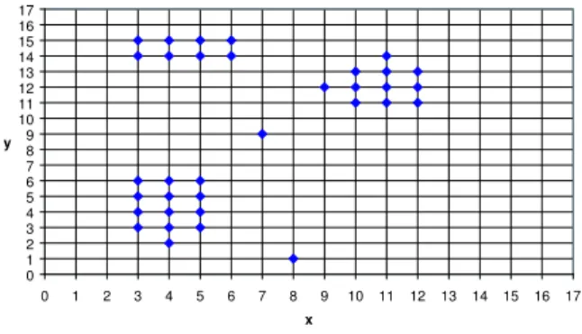
We shall illustrate fpMAFIA with the following set of data points in a two-dimensional space S in Figure 1. Both dimensions are continuous and range from 0 to 17 inclusive. For simplicity, the data points are assumed to have only integer values. There are 34 points in total and each of the points are represented by a diamond in Figure 1. 0 1 2 3 4 5 6 7 8 9 10 11 12 13 14 15 16 17 0 1 2 3 4 5 6 7 8 9 10 11 12 13 14 15 16 17 x y
Figure 1: Sample data setS in 2-D feature space
3.1.2 Adaptive Grid
The Adaptive Grid Algorithm is adopted from pMAFIA, and includes some modifications to suit our application. The goal of the algorithm is to divide each dimension into unequal partitions based on the data distribution. These adaptive intervals are the basis of the frequent baskets, and determine the for-mation and the boundary of the clusters. In our adop-tion of pMAFIA, all parameters and constants are chosen to be the same set of values used in pMAFIA unless stated otherwise.
Let D ={d1, d2, d3, ...} denote the set of
dimen-sions in the feature space. For each dimension di where i denotes the ith dimension, it is divided up into small equi-length partitions calledfine bins(bi,j), where j denotes the jth bin in the dimension. Let
vi,mindenote the minimum value in dimensiondiand vi,max denote the maximum value in dimension di, then the number of fine bins in dimensiondi is given in Formula 1.
|bi|=max(1000, vi,max−vi,min) (1) The algorithm repeats the process for every dimen-sion in the feature space. After the process is finished, the algorithm reads the data once and increments the frequency of a fine bin if a data point falls in the range of the fine bin. Starting form the first fine bin, a set of five consecutive fine bins then from awindow w:
wi,j:bi,j∪bi,j+1∪bi,j+2∪bi,j+3∪bi,j+4,j <|bi| ∧5|j The largest histogram value among the fine bins is taken to represent the value of the window:
v(wi,j) = max(histogram value(bi,k)), k≤j < k+ 4 The algorithm then examines adjacent windows and merges the windows if the values of the windows differ by less than a percentage β. In pMAFIA, β is chosen to be 20%. Let wi,jm denote a merged
win-dow, and let v(wi,j) denote the value of windowwi,j, expressing the idea mathematically:
wi,mj :wi,j∪wi,j+1,if 1−β < v(wi,j+1)/v(wi,j)<1+β
The value of the merged window is the average of all the combined windows. The process is repeated until the algorithm examines all the windows in all the dimensions. The windows then become the adaptive grid bins g.
If the data in any particular dimension is uniformly distributed, then most likely the algorithm returns only one adaptive grid that consisted of the whole dimension. We need to examine such a dimension further to make sure that it does not contribute to any potential clusters. We split the dimension into five equi-length partitions.
We need to determine whether the adaptive grids are worth investigating. Hence we calculate a thresh-old t for each adaptive grid bin to distinguish the dense adaptive grid bins from the sparse ones. For dense bins, we expect them to contain more data points with respect to their sizes. The threshold is defined as in Formula 2.
ti,j = αai,jN
Di
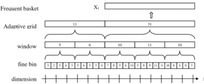
(2) where ai,j is the range of the bin,Di is the range of the dimension that the bin belongs to and N is the total number of points in the data set. The density factor α quantifies the density of the bin, and the value is chosen be 1.5 in pMAFIA. For the uniformly distributed dimensions mentioned earlier, their den-sity factor is lowered toα= 0.9 in our adoption of the algorithm for further examination. If the frequency of the adaptive grid bins exceeds the threshold, the algorithm reports them asfrequent baskets f. The hi-erarchy of the entities in the algorithm is illustrated in Figure 2.
As mentioned before, we adopted the Adaptive Grid Algorithm from pMAFIA but it has certain lim-itations and inherent ambiguity. For example, it does not specifically deal with dimensions that have only a limited set of discrete and unrelated values and im-plicitly assumes that all continuous dimensions have fractional values. Hence we make the following exten-sions to the algorithm in order to make it work with such types of data sets.
x 5 4 6 10 11 10 3 2 5 31 11 6 5 3 5 3 4 7 8 5 6 10 5 8 9 114 10 8 4 9 3 X1 Frequent basket Adaptive grid window fine bin dimension
Figure 2: Hierarchy of Entities
For binary and discrete attributes, we map the val-ues to integers and treat them as continuous dimen-sions. The range of the dimension is equal to the number of discrete values in the attribute. Therefore the number of bins for these dimensions is also equal to the range of the dimension, and the bins become the adaptive grid bins directly without any merging. After some initial analysis on the data set, we char-acterise the numeric attributes into two categories:
1. attributes that represent a percentage (which only ranges from 0% to 100%), or attributes with integer values and range in the hundreds 2. attributes with integer values and ranges in the
millions.
Following the original algorithm to process these two categories of the attributes is inefficient and makes little sense. For the first type of attribute, it is mean-ingless to split the dimensions into 1000 fine bins since the fine bins between the significant values contain no data points. In other words, for the attributes of per-centage type there are only 101 possible significant values (from 0% to 100% inclusive). The majority of the fine bins will have a zero frequency count and defeat the purpose of the adaptive grid bins. Instead of dividing into fine bins, we allocate enough bins for all the significant values in the dimension. The bins then turn into windows directly and these windows may merge to form adaptive grid bins.
For the second type of attributes, it is memory-intensive to allocate the number of fine bins required, and the possible number of frequent baskets reported is large. Therefore if the size of the dimension exceeds a predefined large value , we transform all the old valuesvold on a logarithmic scale using Formula 3.
vnew= ln(vold+ 1) (3)
The new values can be mapped into a continuous dimension that the algorithm can process more effi-ciently. We set = 10,000 in our algorithm. Both modifications are illustrated in Figure 3.
ln(y+1) 5 9 7 6 2 0 8 fine bin window 5 9 7 6 2 0 8 dimension x 1 2 3 4 5 6 7 0 0 y 1,000,000 13.82
1. attributes range in hundreds 2. attributes range in millions
Figure 3: Modification of the Adaptive Grid Algo-rithm
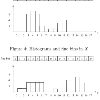
It is best to illustrate the algorithm using the sam-ple data spaceSearlier to see how it works. Since we are working with a small set of data, we increase the value ofβfrom 20% to 50% to better illustrate the al-gorithm. The range of the both dimensions is [0,17], the algorithm allocates 18 fine bins and these fine bins
6 1 2 3 4 5 6 7 8 9 10 11 12 13 14 15 16 17 0 x 4 2 0 0 6 7 6 2 1 1 1 3 4 3 0 0 0 0 0 fine bin 0
Figure 4: Histograms and fine bins inX
6 1 2 3 4 5 6 7 8 9 10 11 12 13 14 15 16 17 0 y 4 2 0 1 1 3 3 3 3 0 0 1 0 3 4 3 5 4 0 fine bin 0
Figure 5: Histogram and fine bins inY
with their frequency counts are illustrated in Figure 4 and Figure 5.
Since the ranges of both dimensions is small, the fine bins are turned into windows directly. Starting fromX, the first three windows are merged since they have the same count of zero points. The fourth win-dow is merged with the fifth winwin-dow because the dif-ference in value is 25% and is within the thresholdβ. The sixth window is merged in a similar fashion. The seventh window is not merged since the difference is larger than the threshold. The process continues for the remaining windows and also for dimensionY. The resulting adaptive grid bins are illustrated in Figure 6 and Figure 7. 0 0 6 7 6 2 1 1 1 3 4 3 0 0 0 0 window 0 0 19 2 3 10 0 adaptive grid 0
Figure 6: Adaptive grid bins inX
Using the formula 3, we calculate the threshold for the adaptive grid bins. For example, the threshold for the second adaptive grid bin is equal to 1.5×3×34
17 = 9.
Since the frequency of this bin is 19, it is reported as a frequent baskets. Repeating the procedure for all the adaptive grid bins, we find in total five adaptive grid bins that are dense and we report them as the frequent baskets. We shall name the first frequent basket found in dimensionX asx1and other baskets
in similar fashion. Therefore the complete set of fre-quent baskets with their frequency count isF = [x1:
19, x2: 10,y1: 12,y2: 10,y3: 9 ].
3.1.3 Frequent-Pattern Tree
As mentioned in Section 2.2.3, the approach proposed in both CLIQUE and pMAFIA is similar to the Apri-ori algApri-orithm (Agrawal & Srikant 1994) used in min-ing association rules. Hence both algorithms have a time complexity of O(ck) where k is the highest di-mensionality of the clusters and c is some constant. To overcome this problem, we need a different ap-proach. FP-growth is a recently proposed method for mining frequent itemsets and we wish to employ the
0 1 1 3 3 3 3 0 0 1 0 3 4 3 5 4 0
window 0
0 2 12 0 1 10 9
adaptive grid 0 0
Figure 7: Adaptive grid bins in Y
fundamental idea of the FP-growth algorithm in our clustering algorithm.
The set of frequent baskets that we obtained ear-lier can be thought of as the equivalent of frequent items in a transaction database. Therefore if the value of a data point falls inside the range of one of the fre-quent baskets, the data point can be thought as a record that contains the frequent item. If we repeat the process for all the attributes, we are able to trans-form any data points to a set of frequent baskets.
If we transform the entire data set to a set of records with various numbers of frequent baskets, the problem of finding clusters becomes the equivalent of mining the frequent itemsets in a database of transac-tions. Ak-dimensional clusterC is thus akfrequent itemset. Using the FP-tree we can efficiently mine these frequent itemsets.
Letp= (p1, p2, p3, ...) denote a data point in the
data setSandF ={f1,1, f1,2...}be the set of frequent
baskets. If we define a functionγas:
γ(pi, fi,j) =
1 pi lies within the range offi,j
0 pi does not lay within the range offi,j Then we can define a transformation Γ onpfor all dimensions as:
Γ(p, F) =
∅ γ(pi, fi,j) = 0,∀fi,j in F fi,j γ(pi, fi,j) = 1
After the transformation Γ, we obtain the set of frequent baskets. We sort the set based on the fre-quency of the frequent basket from the most frequent to the least frequent. Apply the transformation for all the data points in S and we obtain sets of fre-quent baskets representing the entire data set. We can construct the FP-Tree accordingly.
We construct the FP-tree as described in (Han et al. 2000) with the subtle difference that we do not maintain the node-link (a pointer to the next node in the FP tree carrying the same frequent item). There are two reasons for the change:
1. Using the node-link to recover other clusters will yield many subspace projections of the set of high dimensional clusters in which we are not inter-ested.
2. One of the requirements of the clustering algo-rithm is to cover over 95% of the data set. Us-ing the original method specified in FP-growth to mine the frequent itemsets will not guarantee that we will meet this requirement.
We shall continue our discussion with the data set
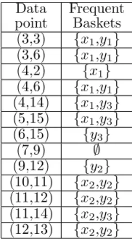
Sto illustrate the construction of the FP-Tree. After we obtain the set of frequent basketsF, we sort the set in the order of descending frequency count. Hence the new set is F0
= [ x1: 19, y1: 12, x2: 10, y2: 10,
y3: 9 ]. We transform the data points into sets of
frequent baskets and sort them inF0
order. Some of the transformations are shown in Table 1.
After the transformation, we construct the FP-Tree according to description in (Han et al. 2000). The final FP-Tree is shown in Figure 8.
Data Frequent point Baskets (3,3) {x1,y1} (3,6) {x1,y1} (4,2) {x1} (4,6) {x1,y1} (4,14) {x1,y3} (5,15) {x1,y3} (6,15) {y3} (7,9) ∅ (9,12) {y2} (10,11) {x2,y2} (11,12) {x2,y2} (11,14) {x2,y3} (12,13) {x2,y2}
Table 1: Transformation of points into frequent bas-kets root y3: 1 x2: 10 y3: 6 y1: 12 y3: 2 x2: 1 y2: 11 x1: 19
Figure 8: FP-Tree forS
3.1.4 Cluster Recovery using Count Back According to the rule of monotonicity stated in (Agrawal et al. 1998), a k-dimensional cluster C is also a cluster in any (k−1)-dimensional subspace pro-jection. Therefore it is conceivable that we will find many frequent itemsets that describe only a few dis-tinct clusters. Moreover, we need a method to recover the clusters such that the clusters cover the majority of the data set. Therefore we devise a new method to recover the clusters from our FP-Tree.
Algorithm 1 describes our method in detail: Algorithm 1 Cluster Recovery using Count Back Method
while there are nodes under root node not pro-cessed do
if current node still has unprocessed children nodes then
traverse down to next level else
if the number of points in the node> κ then label node as a potential cluster
deduct the number of points in the node from all its parent nodes
mark node as processed else
remove node from tree end if
end if end while
The pruning thresholdκ, a percentage of the data set, determines whether a node in the tree has re-ceived enough support. If it has enough support, it will be labelled as a “cluster” node. The threshold
κdirectly determines the number of data points that
are covered by the clusters and the classification of data points. If κ is large, we expect that a lot of nodes in the tree are pruned and the resulting set of clusters do not cover as much as the data set as we want. Similarly ifκis small, a lot of nodes that should be pruned away will be marked as potential clusters. We varied κbetween 0.5% to 50.0% of the data set for the purpose of evaluation which we shall describe in Section 4.3.
Once the algorithm has processed the entire FP-Tree, we can determine the clusters using a straight-forward method. First we traverse the tree from the root node to find the nodes that have been marked as a “cluster” node. The cluster is represented by the set of frequent baskets along the path from the root to the “cluster” node. When we find one of these nodes, we traverse back up the FP-Tree and report the clus-ter. Any subsequent branches under the “cluster” node are ignored since they are part of the reported cluster.
A simple method to determine a “cluster” node is to compute a threshold for every node in the tree. The threshold will be a function of the frequent bas-ket it carries and the depth of the node in the tree. If the number of points in the node exceeds the thresh-old, then it is flagged as a “cluster” node. Neverthe-less we cannot guarantee the number of points that the resulting clusters will cover. With the count back method, we have more control over the coverage of the clusters on the data set using the thresholdκ. There-fore the count back method is the better alternative under this restriction.
The rationale of the count back method is that we do not want to discriminate heavily supported nodes that are high up in the tree. The children nodes may receive enough support themselves to be classified as a “cluster” node, however we want to make sure the eventual clusters can cover enough points in the data set.
Continuing our demonstration with the FP-Tree constructed from the data set S, we set κ = 15% which is equal to 5.1 data points. The first iteration of the algorithm marks the nodes{x1,y1},{x1,y3}, and
{y2,x2}as the “cluster” nodes since their frequency
count exceeds the required percentageκ. The nodes
{x2,y3} and {y3} are under the threshold and they
are removed. Once these “cluster” nodes are marked, we deduct the number of points inside the “cluster” nodes from their parents. The resulting FP-Tree is shown in Figure 9.
root
x2: 1
y2: 1
x1: 1
Figure 9: FP-Tree after first iteration of count back method
All of the nodes left in the tree are under the threshold and hence they are pruned away. We reach the terminating condition of the “while” loop. Using the frequent baskets, the algorithm determines the range of the clusters and returns the following set of clustersC:
c1:{3≤x≤5,3≤y≤6},
c2:{3≤x≤5,14≤y≤15},
3.1.5 Duplicate Clusters Removal
Once we obtain the set of the clusters, it is possible that the set is notorthogonal, i.e., some clusters have extended in more dimensions than other clusters. Al-though the method of the recovery of clusters has eliminated most of them, they can still be reported as a result of the structure of the FP-Tree. This is because identical branches are possible at different levels of the FP-tree. If they both exceed the thresh-old κ, the algorithm reports both the branches that made up the cluster.
To eliminate the sub-clusters (reported clusters that have extended in more dimensions than other clusters), Algorithm 2 describes the steps in detail. Algorithm 2Sub-cluster Elimination
sort the set of clustersCin order of the least num-ber of dimensions first
fori= 0 to (length of set - 1) do forj=i+ 1 to (length of set)do
if cluster[j] is a sub-cluster of cluster[i] then remove cluster[j]
end if end for end for
From the set of clustersC, there are no duplicate clusters. Therefore we shall illustrate the part of the algorithm with another simple example. A FP-Tree
F0
is shown in Figure 10. The corresponding set of clusters is C2 = [{x1,y1},{x1,y2},{y2}]. Following
the elimination algorithm, we sort the clusters and obtain the set C0
2 = [{y2},{x1,y1},{x1,y2}]. Then
starting from the first cluster {y2}, we examine the
subsequent two clusters. Since the last cluster{x1,y2}
is a sub-cluster of{y2}, we remove it from the set. It
leaves us only two clusters in the set and the algorithm terminates. root y1: 6 y2: 8 y2: 6 x1: 15
Figure 10: Example of FP-TreeF0
3.2 Complexity Analysis
The time complexity of the algorithm is dependent on three stages of execution of pfMAFIA: (1) the discov-ery of frequent baskets and the transformation of data points into sets of frequent baskets, (2) the building and the mining of the clusters from the FP-Tree, and (3) the elimination of sub-clusters.
To find all the frequent baskets, fpMAFIA requires two passes of the data set. The first pass determines the range of the dimensions and the second pass de-termines the histogram count of the fine bins in the dimensions. To transform the data points into fre-quent baskets, fpMAFIA requires another pass of the data set. Thus, the time complexity of the first stage is O(N), whereN is the total number of data points in the data set.
To analyse the complexity of the second stage, we first make the following definitions. Let Nf b denote the number of frequent baskets found,Nd denote the total number of dimensions in the feature space, and
Nd(f b) denote the total number of dimensions that
contain frequent baskets. In other words, if there are
ndimensions in the feature space but frequent baskets are found only in m dimensions, then Nd(f b) = m.
ThereforeNd ≥Nd(f b). We define µ as the average
number of frequent baskets per contributing dimen-sion, henceµ= Nf b
Nd(f b) andµ≥1. We shall consider
the average case first then the worst case.
We assume that: (1) each level of the tree contains frequent baskets from only one of the dimensions in the feature space, and (2)Nd(f b)=Nd. The compu-tational complexity of any operations performed on the tree is dependent on the size of the tree. Follow-ing the assumptions above, thenth level of the tree
containsµn nodes. Since there areN
d levels in the tree, the total number of the nodes isO(µNd). 3
The worst case analysis is different to the average case. The first assumption is no longer valid, but we first consider the special case that every dimension contains only one frequent basket, hence Nf b = Nd andµ= 1. First all allowable combinations of the fre-quent baskets are presented and hence the FP-Tree is populated with many nodes and branches to fit these combinations. We shall consider the frequent basket that ranked lowest (fNf b). Given a set of n
frequent baskets, the total number of possible combi-nation withfNf bis
Nf b−1 n−1
. Therefore the total number of possible combinations withfNf bis the sum
of all combinations of the set of frequent baskets from zero to the number of frequent basketsNf b.
Nf b−1 X i=0 Nf b−1 i = 2Nf b
Therefore the number of nodes that carryfNf b is
2Nf b. Similarly, counting the possible number of
com-binations for the second lowest ranked frequent basket (without fNf b), we know that the number of nodes
that carry the frequent basket is 2Nf b−1. Extending
the arguments for other frequent baskets, we can pre-cisely compute the size of the tree which is equal to 2Nf b+1. In our special case whereNf b=Nd, the size
is also equal to 2Nd+1. The result implies that the size
of the tree is exponential to the number of dimensions in the data set.
We then consider the general case of µ >1. The number of nodes carryingfNf bincreases by some
con-stant factor as the number of possible combinations with fNf b increases. The size of the tree increases
and the size complexity becomesO(cNd+1), where c
is some constant. Therefore both the operations that involve the FP-Tree will also have a computational complexityO(cNd+1).
The time complexity of the third stage isO(n2
c), where nc denote the number of clusters discovered. Neverthelessncis usually very small compared to the number of frequent baskets found.
Therefore the worst case complexity of fpMAFIA isO(N+cNd+1+n2
c). The complexity suggests that the algorithm does not scale well with an increase in dimensions, but our empirical results demonstrate that the parameter values in practice are quite small,
3
The sum of the finite geometric series:Pn−1
i=0r
i= rn−1
e.g. c= 1.32. The time complexity for both CLIQUE and pMAFIA are O(N k0
+ck0
), wherek0
denote the maximum dimensionality of the cluster. Therefore these algorithms are more susceptible to high dimen-sional clusters. Not only do they need more passes of the data, the number of candidate dense units gen-erated also grows exponentially. Comparatively our algorithm is able to handle clusters that have high dimensions more gracefully, i.e., without any extra passes on the data and no candidate dense units are generated.
4 Evaluation
4.1 Description of the DARPA Data Set The data used for testing is the KDD Cup 1999 data mining competition data set (KDD 1999). It orig-inated from the 1998 DARPA Intrusion Detection Evaluation Program managed by MIT Lincoln Labs. Lincoln Labs simulated a military LAN and peppered it with multiple attacks over a nine week period. The training data set consists of the first seven weeks of traffic with around 4.9 million connections and the testing data consists of the last two weeks of traf-fic with around 300,000 connections. It contains new types of attack that were not present in the training data.
The entire data set was generated by collecting the binary TCP dump and converting them to a series of connection records. Each record consisted of 41 fea-tures of various types, and a class label that is either “normal” or one of the attack types. The types of attack include denial of service, unauthorized access and probing attacks.
The extracted features included the basic features of an individual TCP connection, content features within a connection suggested by domain knowledge, and traffic features computed using a two-second time window.
4.2 Experimental Setup
In our experiment, we did not use all the data from the 1999 KDD Cup data set. Since it was a super-vised learning competition, the data set contains a high percentage of attack traffic for training purposes. We need to filter out most of the attacks however to fit Assumption 1. When the filtering is done, all 24 types of attack that are presented in the original training data set are equally represented (as much as possi-ble) in the training set we used. It contains around 1 million records.
The testing data set also has a similar problem, and we perform more filtering. Upon close exam-ination, two types of DoS attacks constitute just over 71% of the testing data sets. There are smurf and neptune attacks that are easily detectable by other means (Abdelsayed, Glimsholt, Leckie, Ryan & Shami 2003) since they generate large volumes of traffic. Removing these attacks from the testing set prevents the result being heavily biased and enhances its meaning. As a result, the testing data set only contains around 80,000 records.
The parameter values used by our algorithm are shown in Table 2.
After the training phase is completed, we obtain a set of clusters. Our assumption is that only the points that fall outside of the boundary of these clusters is classified as anomalies. Therefore using the same as-sumption, we labelled the test data in the same man-ner. If the test data point falls outside of the bound-ary of any clusters, it is labelled as an anomaly.
Parameter Value
α 1.5
β 20%
10,000
κ 0.5% – 50.0%
Table 2: Various values of parameters in pfMAFIA 4.3 Results
The pruning thresholdκdetermines the resulting set of clusters that the algorithm produced. We can eval-uate the performance by varying the threshold and obtaining different unique sets of clusters. From these clusters we obtained the corresponding false positive rate and detection rate. We use the results gathered to plot the ROC graph in Figure 11.
0 10 20 30 40 50 60 70 80 90 100 0 20 40 60 80 100
False Positive Rate (%)
D et ec tio n R at e (% )
Figure 11: ROC curve of pfMAFIA
For comparison, we obtained a set of similar ROC graphs from (Eskin et al. 2002) and (Oldmeadow et al. 2004). The curves were produced using the same data sets, but with different clustering or out-lier mining techniques. In (Eskin et al. 2002), Stolfo, et al. evaluated thek-Nearest Neigbhour outlier min-ing algorithm (K-NN), fixed-width clustermin-ing algo-rithm (Cluster) and support vector machine (SVM). In (Oldmeadow et al. 2004), Oldmeadow, et al. evalu-ated the modified clustering-TV algorithm (Modified Cluster-TV). 0 10 20 30 40 50 60 70 80 90 100 0 20 40 60 80 100
False positive rate (%)
D et ec tio n ra te (% ) Modified Cluster-TV Cluster K-NN SVM
Figure 12: ROC curves from Stolfo, et al. and Old-meadow, et al.
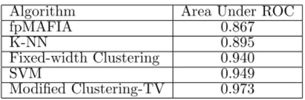
Let Area(R) denote the area under the Receiver Operator Characteristic (ROC) curve R. To more accurately compare these approaches, we calculated the performance value using the area under the ROC curves in Figure 11. We also show the area under the ROC graphs in Figure 12 and presented both sets of figures in Table 3. The conditions which the ROC
graphs are produced are slightly different, however the comparison is still meaningful.
Algorithm Area Under ROC
fpMAFIA 0.867
K-NN 0.895
Fixed-width Clustering 0.940
SVM 0.949
Modified Clustering-TV 0.973 Table 3: Comparison of Performance
It is worth mentioning the experimental setup of which the results are obtained in the studies by Stolfo, et al. (Eskin et al. 2002) and Oldmeadow, et al. (Oldmeadow et al. 2004), such that the comparisons between results from Table 3 are more meaningful. Although Stolfo, et al. did filter most of the attack from the training set to fit Assumption 1, they failed to describe how the filtering was done. Moreover, they used primarily the training data for both testing and training of the algorithm. As mentioned in Sec-tion 4.1, the testing data contains new type of attacks that are not presented in the training data. There-fore their algorithms would have “seen” all the attacks during the testing phase whereas our algorithm would have not “seen” such attacks. The testing codition of the experiments by Oldmeadow, et al. is roughly the same as ours. Nevertheless their algorithm has the added advantage that it used hand-crafted fea-ture weighting to improve its detection rates in some DoS attacks.
5 Discussion
Our results indicate that while fpMAFIA was able to achieve a high detection rate, it suffered from a high false positive rate compared to the other meth-ods. Table 3 showed that the performance value of fpMAFIA is 0.867. It is approximately 3% – 12% worse off than the other algorithms.
Further analysis reveals that pfMAFIA reports only one cluster under various values ofκ. The nature of the cluster remains the same, with the number of dimensions in the cluster varying with different values ofκ. Nevertheless there is no correlation between the two values.
Interpreting the cluster in human readable form reveals that the majority of the connections share exactly the same values in a set of features. Thise set includes a large number of content features (e.g., number of “su root” commands attempted, number of failed logins, number root shells obtained, etc.), a few basic features (number of wrong fragments, number of urgent packets, and number of connections from/to the same host/port) and a moderate number of de-rived features (percentage of connections that have “SYN” errors, percentage of connections that have same or different service, etc.). Therefore the result suggests that this set of features is important in classi-fying the nature of the TCP connections. As shown in Figure 11, the connection is more likely to be normal if it meets all the conditions described by the cluster. Providing the data set is an accurate representative of the real world, a more simple and effective intru-sion detection scheme can be designed with particular focus on these features.
Nevertheless the lack of multiple clusters is one of the possible reasons for the inaccuracy of fpMAFIA in comparison to algorithms tested in (Eskin et al. 2002) and (Oldmeadow et al. 2004). Both studies used the fixed width clustering algorithm described in Sec-tion 2.2.1 as their unsupervised anomaly detecSec-tion
algorithm. Compare to our density and grid-based clustering algorithm, the fixed width clustering algo-rithm has the added advantage that it can cluster ev-ery point in the data set. Therefore the anomalies are clustered into a set of small clusters and their identifi-cation are more straightforward. On the other hand, the density-based clustering algorithm has the inher-ent inability to cluster points that lay in sparse region of the data space. Since the anomalies only make up a small percentage of the data set, which are the most likely occupants of the sparse regions according to Assumption 2, most are ignored. The results sug-gested thatthe identification of the precise nature of anomalies is an important factor on the performance of unsupervised anomaly detection algorithm in net-work intrusion detection.
Although we obtained the ROC graphs under dif-ferent conditions compared to the experiments set up in (Eskin et al. 2002) and (Oldmeadow et al. 2004), our results compare only slightly unfavourably against them. Given the empirical run time statis-tics of pfMAFIA, we consider the algorithm has been reasonably sucessful, and is a promising subject of further research for high dimensional datasets.
6 Further Work
There are a few areas of the project that we suggest as topics for further work:
• We acquired the values of the parametersαand
β from the adaptive grid algorithm in pMAFIA. The choice of these parameters, however, may affect the accuracy of the final results. We would like to investigate the possible effects in changing the values ofαandβ independently in detail.
• We argue that the pruning threshold κ deter-mines the number of points that the resulting set of clusters will cover. Nonetheless it does not appear to be the case with this data set. There is correlation between the two values but no obvi-ous proportionality relationship. We would like to further examine the exact effects of varyingκ
and the number of points that the clusters cover.
• We would also like to improve upon the current pfMAFIA in several directions. One possible direction is substituting the mining of frequent itemsets with the mining of maximally frequent itemsets. Thus, the clusters will always have the highest dimensions possible. This may contra-dict our aim of maximum coverage but we may be able to make some modifications of the algo-rithm to achieve both aims.
7 Conclusion
We have evaluated a new approach in unsupervised anomaly detection in the application of network in-trusion detection. The new approach, fpMAFIA, is a density-based and grid-based high dimensional clus-tering algorithm for large data sets. It has the ad-vantage that it can produce clusters of any arbitrary shapes and cover over 95% of the data set with ap-propriate values of parameters. We provided a de-tailed complexity analysis and showed that it scales linearly with the number of records in the data set. We have evaluated the accuracy of the new approach and showed that it achieves a reasonable detection rate while maintaining a low positive rate. Using the results, we provided some insights to the likely requirements of a good unsupervised anomaly detec-tion scheme in the applicadetec-tion of network intrusion detection systems.
Acknowledgements
We thank the organisers of the 1999 KDD Cup for the use of their datasets. This work was supported in part by the Australian Research Council.
References
Abdelsayed, S., Glimsholt, D., Leckie, C., Ryan, S. & Shami, S. (2003), An efficient filter for denial-of-service bandwidth attacks. In Proceedings of IEEE GLOBECOM-03, pp. 1353–1357.
Agrawal, R., Gehrke, J., Gunopulos, D. & Raghavan, P. (1998), Automatic subspace clustering of high dimensional data for data mining applications. InProceedings of SIGMOD 1998, pp. 94–105. Agrawal, R. & Srikant, R. (1994), Fast algorithms for
mining association rules. In Proceedings of 20th International Conference of Very Large Data Bases (VLDB), pp. 487–499.
Ankerst, M., Breunig, M. M., Kriegel, H.-P. & Sander, J. (1999), ‘Optics: ordering points to identify the clustering structure’. In SIGMOD Rec.28(2), 49–60.
Denning, D. (1987), ‘An intrusion detection model’. In IEEE Transactions on Software Engineering 13.
Eskin, E. (2000), Anomaly detectino over noisy data using learned probability distributions. In Pro-ceedings of the International Conference on Ma-chine Learning (ICML 2000).
Eskin, E., Arnold, A., Prerau, M., Portnoy, L. & Stolfo, S. (2002), A geometric framework for un-supervised anomaly detection: Detecting intru-sions in unlabeled data. InApplications of Data Mining in Computer Security.
Ester, M., Kriegel, H.-P., Sander, J. & Xu, X. (1996), A density-based algorithm for discovering clus-ters in large spatial databases with noise. In Pro-ceedings of KDD-96, pp. 226–231.
Gonzalez, F. & Dasgupta, D. (2002), Neuro-immune and self-organizing map approaches to anomaly detection: A comparison. In Proceedings of the 1st International Conference on Artificial Im-mune Systems, pp. 203–211.
Gonzalez, F. & Dasgupta, D. (2003), Anomaly de-tection using real-valued negative selection. In Genetic Programming and Evolvable Machines, Vol. 4, pp. 383–403.
Han, J., Pei, J. & Yin, Y. (2000), Mining frequent patterns without candidate generation. In Pro-ceedings of the 2000 ACM SIGMOD Intl. Con-ference on Management of Data, ACM Press, pp. 1–12.
Hipp, J., G¨untzer, U. & Nakhaeizadeh, G. (2000), Algorithms for association rule mining – a gen-eral survey and comparison. InSIGKDD Explo-rations2(1), 58–64.
Javitz, H. S. & Vadles, A. (1993), The NIDES statis-tical component: Description and justification. Technical report, SRI International.
KDD (1999), The third international knowl-edge discovery and data mining tools
competition dataset (KDD99 Cup).
http://kdd.ics.uci.edu/databases/kddcup99.html.
Lane, T. & Brodley, C. E. (1997), Sequence matching and learning in anomaly detection for computer security. In Proceedings of the AAAI Workshop on AI Approaches to Fraud Detection and Risk Management, AAAI Press, pp. 43–49.
Laskov, P., Schafer, C. & Kotenko, I. (2004), Intru-sion detection in unlabeled data with quarter-sphere support vector machines. InDetection of Intrusions and Malware & Vulnerability Assess-ment (DIMVA), Dortmund.
Lazarevic, A., Ertoz, L., Kumar, V., Ozgur, A. & Srivastava, J. (2003), A comparative study of anomaly detection schemes in network intrusion detection. InProceedings of the Third SIAM In-ternational Conference on Data Mining.
Lee, W. & Stolfo, S. (1998), Data mining approaches for intrusion detection. In Proceedings of the 7th USENIX Security Symposium (SECURITY ’98).
Nagesh, H. S., Goil, S. & Choudhary, A. N. (2000), A scalable parallel subspace clustering algorithm for massive data sets. In Proceedgins of th In-ternational Conference on Parallel Processing, p. 477.
Noble, C. & Cook, D. (2003), Graph-based anomaly detection. InProceedings of KDD-03.
Oldmeadow, J., Ravinutala, S. & Leckie, C. (2004), Adaptive clustering for network intrusion detec-tion. In Proceedings of the Third International Pacific-Asia Conference on Knowledge Discov-ery and Data Mining (PAKDD 2004).
Portnoy, L., Eskin, E. & Stolfo, S. (2001), Intrusion detection with unlabeled data using clustering. InProceedings of ACM CSS Workshop on Data Mining Applied to Security (DMSA-2001). Sheikholeslami, G., Chatterjee, S. & Zhang, A.
(1998), WaveCluster: A multi-resolution cluster-ing approach for very large spatial databases. In Proceedings of the 24th International Conference of Very Large Data Bases (VLDB), pp. 428–439. Shyu, M.-L., Chen, S.-C., Sarinnapakorn, K. & Chang, L.-W. (2003), A novel anomaly detection scheme based on principal component classifier. InProceedings of the IEEE Foundations and New Directions of Data Mining Workshop.
Wang, W., Yang, J. & Muntz, R. R. (1997), Sting: A statistical information grid approach to spatial data mining. In Proceedings of the 23rd Inter-national Conference on Very Large Data Bases, Morgan Kaufmann, pp. 186–195.
Zanero, S. & Savaresi, S. (2004), Unsupervised learn-ing techniques for an intrusion detection system. In Proceedings of the ACM Symposium on Ap-plied Computing, ACM SAC 2004.