Large-Scale Parallel State Space Search
Utilizing Graphics Processing Units
and Solid State Disks
Dissertation
zur Erlangung des Grades eines
Doktors der Naturwissenschaften
der Technischen Universit ¨at Dortmund
an der Fakult ¨at f ¨
ur Informatik
von
Damian Sulewski
Dortmund
2011
Tag der m¨undlichen Pr¨ufung:
Dekanin: Prof. Dr. Gabriele Kern-Isberner Gutachter: Prof. Dr. Stefan Edelkamp
v
Abstract
The evolution of science is a double-track process composed of theoretical insights on the one hand and practical inventions on the other one. While in most cases new theo-retical insights motivate hardware developers to produce systems following the theory, in some cases the shown hardware solutions force theoretical research to forecast the results to expect.
Progress in computer science rely on two aspects, processing information and stor-ing it. Improvstor-ing one side without touchstor-ing the other will evidently impose new prob-lems without producing a real alternative solution to the problem. While decreasing the time to solve a challenge may provide a solution to long term problems it will fail in solving problems which require much storage. In contrast, increasing the available amount of space for information storage will definitively allow harder problems to be solved by offering enough time.
This work studies two recent developments in the hardware to utilize them in the domain of graph searching. The trend to discontinue information storage on magnetic disks and use electronic media instead and the tendency to parallelize the computation to speed up information processing are analyzed.
Storing information on rotating magnetic disk has become the standard way since a couple of years and has reached a point where the storage capacity can be seen as infinite due to the possibility of adding new drives instantly with low costs. However, while the possible storage capacity increases every year, the transferring speed does not. At the beginning of this work, solid state media appeared on the market, slowly suppressing hard disks in speed demanding applications. Today, when finishing this work solid state drives are replacing magnetic disks in mobile computing, and com-puting centers use them as caching media to increase information retrieving speed. The reason is the huge advantage in random access where the speed does not drop so significantly as with magnetic drives.
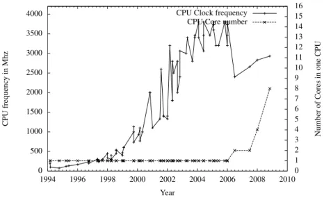
While storing and retrieving huge amounts of information is one side of the medal, the other one is the processing speed. Here the trend from increasing the clock fre-quency of single processors stagnated in2006and the manufacturers started to com-bine multiple cores in one processor. While a CPU is a general purpose processor the manufacturers of graphics processing units (GPUs) encounter the challenge to perform the same computation for a large number of image points. Here, a parallelization offers huge advantages, so modern graphics cards have evolved to highly parallel computing instances with several hundreds of cores. The challenge is to utilize these processors in other domains than graphics processing.
One of the vastly used tasks in computer science is search. Not only disciplines with an obvious search but also in software testing searching a graph is the crucial aspect. Strategies which enable to examine larger graphs, be it by reducing the number of considered nodes or by increasing the searching speed, have to be developed to battle the rising challenges. This work enhances searching in multiple scientific domains like explicit state Model Checking, Action Planning, Game Solving and Probabilistic Model Checking proposing strategies to find solutions for the search problems.
Providing an universal search strategy which can be used in all environments to utilize solid state media and graphics processing units is not possible due to the hetero-geneous aspects of the domains. Thus, this work presents a tool kit of strategies tied together in an universal three stage strategy. In the first stage the edges leaving a node are determined, in the second stage the algorithm follows the edges to generate nodes. The duplicate detection in stage three compares all newly generated nodes to existing once and avoids multiple expansions.
For each stage at least two strategies are proposed and decision hints are given to simplify the selection of the proper strategy. After describing the strategies the kit is evaluated in four domains explaining the choice for the strategy, evaluating its outcome and giving future clues on the topic.
Acknowledgments
In most cases a thesis would not exist without a Ph. D. Supervisor, but in this one the influence of Prof. Dr. Stefan Edelkamp, my supervisor, started much earlier. Being a diploma student he introduced me to the art of Model Checking. I do not know if it was because ofsomeone had to do the jobor because ofyou are the right for the job
but he always motivated me. Prof. Dr. Edelkamp trusted me, much more then I could trust myself, and now you can read the results. Thanks for the endless discussions, on-and off-topic. Thanks for your time whenever I needed it. Thanks for the possibility to find oneself on the long line.
Special thanks go to Prof. Dr. Bernhard Steffen the man with the big picture. Although he never was the one I discussed implementation details with, he was always interested in my work and pushed me in the right direction when I stood at a forking way not knowing where to go. Thanks also for the warm place for my research.
I am also grateful to the other members of the committee: Prof. Dr. Jan Vahrenhold and Dr. Ingo Battenfeld for the help and support in thelast minutes.
Thanks to all the coauthors who showed me the right way to write papers, thanks to Dragan Bosnacki, Pavel ˇSimeˇcek, and especially to Shahid Jabbar. Pavel, perhaps one day we can play a second matchCzech Republic against Poland?
When Stefan is myDoctorvaterthen Shahid certainly is myDoktorbruder. There are two images I see in front of me when thinking about him. I once came into his room and he was working on his thesis, he was adjusting a line in one picture, at the highest zoom level, moving it only some millimeters. It had to be perfect. The other image is a huge number of full and empty boxes in his room. I helped him to transport them to the local UPS store, the evening before his last flight to Sweden. Absolutely chaotic. This made him a human. Staying in the terms of aDoktorfamilieI will never forget my secondDoktorbruderPeter Kissmann. Thanks for destroying my ideas at the right time. Peter is a gifted person in my eyes, his gift is to smell inconsistencies before his discussion partner has formulated the whole idea. It was not always funny to think a whole weekend on a particular algorithm and then see it collapse because of an overseen littleness. And of course thanks for the rigorous proof-reading of this work, I hope it makes it readable.
At this point it is time to thank the whole LS5 Team from the present and the past. I can not remember all the names due to a miserable memory, but i try to remember some. Thanks to the proof readers Julia Rehder, Falk Howar, Maik Merten and Johannes Neubauer. Thanks go to Thomas Wilk for showing me skills in table soccer I will never reach. Thanks to the, sporting ace Christian Wagner for motivation on this domain, and
Sven J¨orges for the photo finish in submitting a dissertation.
All the time during this work, there was only one source of energy for me, this source was, is and will always be my family. I would like to return all of what you gave me, but I am sure I will never be able to. Names given in a text have to be in an order so I order them by age, but trust me Son, Wife, Mom and Dad I did all this for you, for you all.
Last but not least I would like to send special thanks to Cengizhan Y¨ucel a long time student friend and the one of the most reliable persons i ever knew.
Finally a big thanks goes to theDeutsche Forschungsgeselschaftfor financially sup-porting my research through the projectModellpr¨ufung auf Flashspeicher-Festplatte
Contents
1 Introduction 1
1.1 Motivation . . . 1
1.2 State Space Exploration . . . 3
1.2.1 Introducing State Spaces . . . 3
1.2.2 Example of a State Space . . . 6
1.2.3 State Spaces in the Following Parts . . . 7
1.3 Graph Search Algorithms . . . 9
1.3.1 Blind Search . . . 10
1.3.2 External Search . . . 16
1.3.3 Parallel Graph Search . . . 18
1.4 Duplicate Detection in Graph Search . . . 21
1.4.1 Hash Based Duplicate Detection . . . 21
1.4.2 Sorting Based Duplicate Detection . . . 24
1.5 Main Contributions . . . 25
1.6 Organization of the Thesis . . . 26
2 Hardware and Programming Models 29 2.1 Information Storage . . . 29
2.1.1 Random Access and Insufficient Space in Internal Memory . . 30
2.1.2 Pushing Space Constrains by Going External . . . 30
2.1.3 Solid State Disks . . . 30
2.2 Faster Computation Using Parallel Hardware . . . 34
2.2.1 Parallel Computing . . . 34
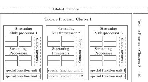
2.2.2 General Purpose Graphics Processors . . . 35
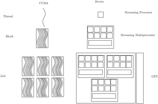
2.2.3 GPGPU Programming Interfaces . . . 36
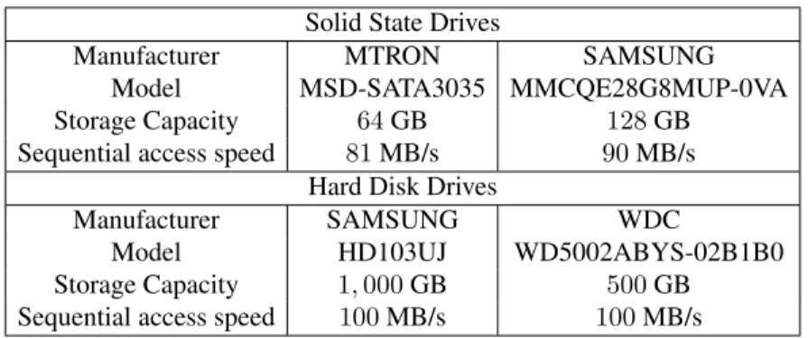
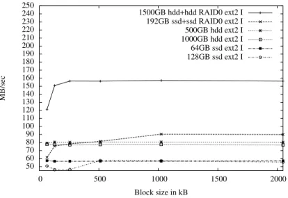
2.3 Used Hardware . . . 43
2.3.1 Solid State Disks . . . 43
2.3.2 Graphics Cards . . . 46
I
Breadth-First Search utilizing Novel Hardware
53
3 Prerequisites for GPU and SSD Utilization 55 3.1 Work Distribution . . . 563.1.1 Independent Limited Memory Tasks . . . 57
3.1.2 Unlimited Memory Tasks . . . 58
3.2 Information Distribution . . . 59
3.2.1 Constant Information . . . 59
3.2.2 Dynamic Information . . . 60
4 GPUSSD - Breadth-First Search 63 4.1 Basic Structure of the Algorithm . . . 63
4.2 Strategies for Successor Generation . . . 65
4.2.1 Successor Counting . . . 65
4.2.2 Successor Pointing . . . 68
4.3 Strategies for Duplicate Detection . . . 71
4.3.1 Sorting Based Duplicate Detection . . . 71
4.3.2 Parallel Hash Based Duplicate Detection . . . 74
4.4 External State Space Exploration on the GPU . . . 76
4.5 Efficient Flat Representation of Formulas . . . 77
4.6 Summary . . . 78
II
Explicit State Model Checking
81
5 Introduction to Explicit State Model Checking 83 5.1 Modeling of Concurrent Systems . . . 845.1.1 Concurrent Systems as Variables and Actions . . . 84
5.1.2 Explicit State Model Checking . . . 85
5.1.3 Explicit State Model Checking Example . . . 86
5.2 Related Work . . . 88
5.2.1 External Explicit State Model Checking Algorithms . . . 88
5.2.2 Parallel Explicit State Model Checking . . . 88
5.3 Summary . . . 89
6 SSD-Based Minimal Counterexamples Search 91 6.1 Semi-External LTL Model Checking . . . 91
6.1.1 Extending to Efficiently Support SSDs . . . 96
6.2 Externalizing the Perfect Hash Function . . . 97
6.3 Summary . . . 98
7 GPU-Based Model Checking 99 7.1 Parsing the DVE Language . . . 99
7.1.1 Checking Enabledness on the GPU . . . 101
7.2 Generating the Successors on the GPU . . . 102
7.3 Duplicate Detection . . . 103
7.3.1 Immediate Detection on (Multiple Cores of) the CPU . . . 103
7.3.2 Delayed Duplicate Detection on the GPU . . . 104
CONTENTS xiii
8 Experimental Evaluation 105
8.1 Results for Semi-External LTL Model Checking . . . 105
8.1.1 Minimal Counterexamples . . . 106
8.1.2 Flash-Efficient Model Checking . . . 106
8.2 Results for GPU-Based Model Checking . . . 108
8.2.1 Evaluation of Immediate Duplicate Detection . . . 108
8.2.2 Experiments with Delayed Duplicate Detection . . . 112
8.3 Summary . . . 114
III
Action Planning
115
9 Introduction to Action Planning 117 9.1 Modeling of Planning Problems . . . 1179.2 PDDL Example of the Thesis Problem . . . 119
9.3 Related Work . . . 119
9.4 Summary . . . 122
10 Action Planning on the GPU 123 10.1 Strategies from the GPUSSD-BFS Framework . . . 123
10.1.1 Successor Generation on the GPU . . . 123
10.2 GPU Planning Algorithm . . . 124
10.2.1 Planner Architecture . . . 124
10.3 Summary . . . 127
11 Experimental evaluation 129 11.1 Results of the Evaluation . . . 129
11.2 Summary . . . 136
IV
Game Solving
137
12 Introduction to Game Solving 139 12.1 Analyzed Games . . . 14012.1.1 Sliding-Tile Puzzle . . . 140
12.1.2 Top-Spin Puzzle . . . 140
12.1.3 Pancake Problem . . . 140
12.1.4 Peg-Solitaire . . . 141
12.1.5 Frogs and Toads . . . 141
12.1.6 Nine-Men-Morris . . . 141
12.2 Game Solving . . . 142
12.3 Related Work . . . 142
13 Perfect Hashing in Games 145
13.1 Properties of State Spaces in Games . . . 145
13.2 Ranking and Unranking in Permutation Games . . . 146
13.2.1 Reducing State Space in Permutation Games . . . 148
13.3 Binomial Coefficient for Single Player Games . . . 149
13.4 Multinomial Coefficient for Multi Player Games . . . 150
13.5 Summary . . . 155
14 GPU Enhanced Game Solving using Perfect Hashing 157 14.1 State Space Algorithms utilizing Perfect Hashing . . . 157
14.1.1 Two-Bit Breadth-First search . . . 158
14.1.2 One-Bit Reachability . . . 159
14.1.3 One-Bit Breadth-First search . . . 159
14.2 Porting Algorithms to the GPU . . . 161
14.2.1 Case Study: Nine-Men-Morris . . . 164
14.3 Summary . . . 167
15 Experimental evaluation 169 15.1 Single-Agent Games . . . 169
15.2 Nine-Men-Morris . . . 171
15.3 Summary . . . 172
V
Probabilistic Model Checking
173
16 Introduction Probabilistic Model Checking 175 16.1 Discrete Time Markov Chains . . . 17516.2 Probabilistic Computational Tree Logic . . . 176
16.3 Algorithms for Model Checking PCTL . . . 176
16.4 Beyond Discrete Time Markov Chains . . . 178
16.5 Summary . . . 178
17 GPU Enhanced Probabilistic Model Checking 179 17.1 Jacobi Iterations. . . 179
17.2 Sparse Matrix Representation. . . 180
17.3 Algorithm Implementation. . . 181
17.4 Extending the Algorithm to Multiple GPUs . . . 184
17.5 Summary . . . 186
18 Experimental evaluation 187 18.1 Verified Protocols . . . 187
18.2 Empirical Results . . . 188
CONTENTS xv
VI
Conclusions and Future Work
193
19 Conclusion 195
19.1 Conclusions . . . 195 19.2 Future Work . . . 198
List of Algorithms
1.1 Graph algorithm using anOpenlist . . . 10
1.2 Graph algorithm using anOpenand aClosedlist . . . 11
1.3 Breadth-First search . . . 12
1.4 Depth-First search . . . 13
1.5 Iterated Depth-First search . . . 14
1.6 Dijkstra’s Algorithm . . . 15
1.7 The External BFS algorithm . . . 17
1.8 Basic parallel search strategy . . . 19
1.9 Hash based parallel search strategy . . . 19
2.1 Matrix Vector Multiplication on the CPU . . . 40
2.2 GPU-Kernelfor the Matrix Vector Multiplication . . . 41
2.3 Host algorithm for the Matrix Vector Multiplication . . . 41
4.1 Basic GPU Parallel Search algorithm . . . 64
4.2 GPU-KernelDetermine Transitions for Successor Counting . . . 66
4.3 GPU-KernelGenerate Successors for Successor Counting . . . 67
4.4 GPU-KernelDetermine Transitions for Successor Pointing . . . 69
4.5 GPU-KernelGenerate Successors for Successor Pointing . . . 70
4.6 GPU-KernelSort buckets in sorting based duplicate detection . . . 73
4.7 GPU-BFS - Large-Scale Breadth-First search on the GPU . . . 77
6.1 Minimal-Counterexample search . . . 93
6.2 BFS-PQFile-based 1-level-bucket priority queue . . . 94
6.3 Prio-min: Synchronized traversal in an1-level-bucket priority queue. . 95
6.4 SSD-LTL-Model-Check: Flash-efficient semi-external Model Checking 97 7.1 GPU-KernelDetermine guard on a given state . . . 102
7.2 GPU-KernelDetect Duplicates via Sorting . . . 102
10.1 Optimal Eager Buffer-Filling GPU Planning algorithm . . . 126
10.2 GPU-KernelGenerate Successors in Planning . . . 127
13.1 unrank(r)with parity derived on-the-fly . . . 147
13.2 Binomial-Rank . . . 150 xvii
13.3 Binomial-Unrank . . . 151
13.4 Multinomial-Rank . . . 152
13.5 Multinomial-Unrank . . . 154
14.1 Two-Bit-Breadth-First search (init) . . . 158
14.2 One-Bit reachability (init) . . . 159
14.3 One-Bit-Breath-First search . . . 160
14.4 One-Bit reachability utilizing the GPU . . . 161
14.5 GPU-KernelDetermine Transitions for One-Bit reachability . . . 162
14.6 GPU-KernelGenerate Successors for One-Bit reachability . . . 163
14.7 BFS for Phase I . . . 165
14.8 Retrograde Analysis Phase I . . . 166
17.1 Jacobi iteration with row compression (as implemented in PRISM) . . 182
17.2 Host part of the Jacobi iteration, for unbounded until . . . 183
17.3 GPU-KernelJacobi iteration with row compression . . . 184
Chapter 1
Introduction
1.1
Motivation
Time is a scarce resource, space is unlimited. This statement is becoming reality in the 64-bit era. Today, an ordinary personal computer utilizes up to 32gigabyte of internal RAM storage, using server hardware even256gigabyte in one computer are possible. Utilizing external storage one can get3terabyte magnetic drives, so called
Hard Disk Drives(HDDs) at nearly100C and continuously falling prices. An example
of resource capabilities these days is the companyGoogle, who is offering an Email service giving each user 7.44gigabyte available space for their mails. In February 2010the service had reported to have170million accounts1with an available space of
1,235,156.25 terabytes or 1.177 exabytes.
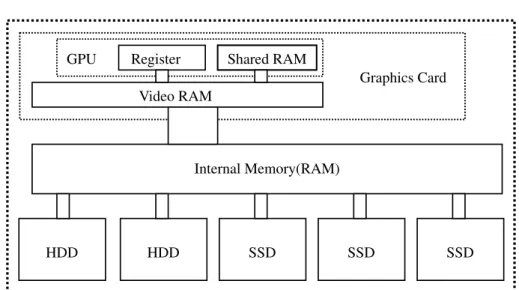
For applications where excessive random access to the data is mandatory and mag-netic drives fail to reach appropriate speeds, solid state drives (SSDs) have entered the market. An SSD stores information on memory chips providing faster access to the data while consuming less power. A system with 256 GB of RAM costs about 4,500 C at today’s prices while the same amount of SSD storage costs nearly300 C utilizing a reading access speed of255MB/s (compared to about100MB/s on HDDs and17GB/s for RAM) and the possibility to be extended by adding more or larger de-vices. The characteristics of solid state media differ significantly from the ones of hard disk devices imposing new challenges on the developers of algorithms. While writ-ing data to such a medium is done at a speed comparable to magnetic devices (bewrit-ing about100MB/s) the reading of random bits can be done with much higher efficiency. These characteristics, additionally with the possibility to even increase the throughput by combining several devices, make them perfect for storing random access structures which exceed the size of RAM.
Rising storage capabilities do not necessarily require a change on the algorithmic level. In contrast to this, the switch from increasing the clock rate to assembling mul-tiple cores in one central processing unit (CPU) demands for a parallelization on the algorithmic level. This change in design forces the algorithms to utilize the available
1http://news.bbc.co.uk/2/hi/8506148.stm
parallel computing power to gain profit from it and requires synchronization techniques and load balancing. The current maximum number of cores in one CPU is8which sim-ulate16cores by utilizing two threads per core. Being confronted with a number of different tasks in parallel, the CPU cores are self-contained computing cores even able to increase the clock for one single core to speed up sequential computation. Simul-taneously to the CPU the developers of the graphics cards increased the computation power by parallelization. Contrary to data processing a graphics processing unit (GPU) is used to compute the visualization for a large number of triangles representing a vir-tual world. Since the triangles are independent and the computation is equivalent for all of them, the parallelization used is the single instruction multiple data (SIMD) tech-nique. Here a large number of processors manipulate data using the same instructions. Current GPUs utilize up to 1,024 processors in one graphics card (NVIDIA GTX 590) and up to4cards can be combined in one system.
This work utilizes recent developments in hardware to solve search problems in which the goal is to find a set of explicit nodes in a graph defined implicitly prior to the search. In animplicit definition just the starting node and atransition function
transforming this node into new ones is given. The main challenge spreading over all implicit graph search problems is thestate space explosion problem, which describes the potentially exponential development of node numbers in the graph. Even small changes in the transition function definition may increase the number of reachable
nodes, on a path from the initial node, dramatically increasing the search time, which is mostly linear to this number.
Between all the available search challenges given in the scientific and non-scientific work, the four investigated domains represent a spectrum and give a starting point for investigation in many other research areas.
The first investigation on the usage of solid state drives and graphics processing units isExplicit State Model Checking(Clarkeet al., 1999; M¨uller-Olmet al., 1999), where the demand for storage space and computation power increased dramatically with the introduction of parallel processors. It should be needless to say how important software verification has become in the last years. With the introduction of concur-rent hardware at affordable prices for everyone, parallel programming has evolved to a standard technique to implement efficient algorithms. Not so long ago, only security related bugs were hunted, or bugs whose removal would directly avoid loosing equip-ment worth millions of dollars like an exploding space rocket. Today all companies search for efficient ways to verify their software because a bug can cause a significant loss of reputation resulting in the emigration of customers. The automobile constructor Mercedes-Benz learned their lesson when long term clients switched to other manu-facturers because of small bugs in the car software. Even though the bugs were not dramatic, e. g., a not opening door when the remote was pressed, the damage to their reputation of being a premium manufacturer was worth millions of dollars due to de-creasing sales.
The second chosen discipline isAction Planning(Russell and Norvig, 2002), where the goal is to find a plan fulfilling predefined conditions given a set of actions. The plan consists of a sequence of transition functions (here denoted asactions) which transform the initial state into a goal state. Prominent examples of planning are logistic domains as well as planning robots which perform various tasks efficiently. This work deals
1.2. STATE SPACE EXPLORATION 3
with deterministic Action Planning where each action is fully defined.
A breadth-first state-space generation in the artificial intelligence (AI) branchGame
Solving (van den Heriket al., 2002) imposes new challenges on the SSD and GPU
utilization. Problems in this domain are usually built up of a high number of available moves, e. g., all possible movements to the figures on a chess board, with only a small number of these being valid moves. While a check for a single move can be done very efficiently the high number of checks imposes a long searching time. An additional aspect of this problems is a large state description where an efficient compression is necessary to traverse the entire state space. Here the computation power of the GPU comes in handy since the decompression and the determination of valid movements can be done in parallel on a huge number of states.
Probabilistic Model Checking(Kwiatkowskaet al., 2007) has been proved to be
a powerful framework for modeling various systems ranging from randomized algo-rithms via performance analysis to biological networks. Although solutions for Proba-bilistic Model Checking can also be obtained by a state space search for a specific state, this is not an efficient way. Here the satisfaction of properties is quantified with some probability in contrast to the previous disciplines. In a state space approach this maps to generating states and annotating them with a probability until the target is reached. Due to the high branching factor it is more efficient to choose a different approach i. e., using numerical methods which enforce different strategies to utilize the GPU and ex-ternal media. In this discipline the GPU has to be used with the intention of solving linear equations, imposing new challenges on the algorithm development.
This work will investigate in using recent developments in hardware to allow for traversing larger graphs in less time in all these domains.
1.2
State Space Exploration
The connecting aspect of all analyzed problems is the traversal of a search graph de-fined only by a starting node and a transformation function. To understand the correla-tion exploited in this work we need to define the basics of thestate space exploration
and present a number of existing algorithms. The following sections will provide the necessary definitions to explore state spaces and to analyze the proposed algorithms.
1.2.1
Introducing State Spaces
As this dissertation concentrates onimplicitlygiven graphs where only a starting point and instructions how to traverse the graph are given we limit the definitions to those graph structures.
Definition 1 (System) A system is a problem definition in a given environment. It includes all the necessary information to solve the problem and can be expressed in a suitable description language.
A system usually consists of three aspects, a description of an environment, defini-tions of transformable elements in this environment and transition funcdefini-tions for these elements. Board games are systems where the board defines the environment and the
pieces are placed or moved by transforming their position. The rulebook defines the transition functions by describing allowed moves.
Definition 2 (State) Astatesis a description representing the overall configuration of a system at a specified point in time.
A state can be the concatenation of sub-states each describing a part of the system. To give an example take a look at the game checkers, here each piece can be a usual
menor aking. One solution to store this difference in a state is to use different notations for this attribute. Another solution is to include this as a special variable representing this piece in the state. This variable is calledlocal statesince a change to this local state is only locally in the whole system.
Definition 3 (Local state) Thelocal stateof an unique actor in a system is a variable describing the current condition of the actor.
As an example, the local state of a piece denotes whether it is a men or a king and a state is the position of all pieces on the board in checkers. Replacing or removing pieces and changing a local state when reaching the appropriate position corresponds to transforming one state into another.
Definition 4 (State Space) Astate spaceS, is the set of all possible configurations of a given system.
The state spaceSof the game chess consists of all the possible placements for all pieces.sinSis mapped to a nodev∈V in the graphG= (V, E).
A subset of all statessˆ∈ S identifies theinitialstates, defined entirely before the search. All systems analyzed in this work only have one single initial state. The set of
reachablenodes is a subsetr⊆ Sdenoting all nodes connected fromˆs.
To define the remaining states the informal definition of the transition function is formalized andtransitions, composed of apreconditionand apostconditionare defined as follows,
Definition 5 (Precondition) A preconditionof a transition defines conditions in the state to be true before transforming the state by applying a transition.
Definition 6 (Transition) Atransitiont in the set of all transitionsT is a pair con-necting one Boolean precondition and a set of postconditions. The transition is called
activewhen the precondition evaluates to true.
A transition has to define the modifications to the state in a set of postconditions. Definition 7 (Postcondition) Thepostconditionsdefine conditions in the state which have to be true after it has been transformed.
A transition froms1 ∈ S tos2 ∈ S is similar to an edge in the directed graph
1.2. STATE SPACE EXPLORATION 5
Both, the precondition and all postconditions may be empty, resulting in a transition applicable to all states or a transition transforming the state into its identity. While the identifier precondition is common in Action Planning the postconditions in Action Planning and Model Checking are calledeffects. The later additionally utilizes the term
guardto denote a precondition. In Game Solving the preconditions are given as rules
whether a move is valid or not, the postcondition is the result of executing a valid move. Probabilistic Model Checking is an exception where all preconditions are active with a given probability. Postconditions are applied when a precondition is chosen.
Definition 8 (Parents and Successors) When applying a transition the base state is
calledparentwhile the resulting state is called successor. Leavesare states without
successors having no active transition.
Definition 9 (Expansion / Generation) During theexpansionof a parent, or the gen-erationof successors, the parent isexpandedwhen all successors have beengenerated.
While definitions so far applied to single nodes in a graph, the following one will cover connected nodes.
Definition 10 (Path) Apathis a sequence of statess0, s1, . . . , snwhere an active
tran-sition exists for all pairs(si, si+1)with0≤i < n. Thelengthof a path isnthe number
of states it contains.
Starting at an initial state and transforming it into a number of successors will generate a tree. To transform this tree into a graph duplicates have to be defined, describing states which are indistinguishable.
Definition 11 (Duplicate) Two statess1ands2reachable on different paths from the
initial state (s . . . sˆ 16= ˆs . . . s2) areduplicateswhen their representations are identical
(writes1=s2).
Lemma 1 In two state spacesS1andS2 using the same set of transitionsT and
du-plicate initial statessˆ1= ˆs2, for each states0∈ S1exists a duplicate states00∈ S2so
thats0 =s00andS1=S2.
Proof.Since the representation of the duplicatesˆs1∈ S1andsˆ2∈ S2are identical the set of active transitionsa⊆T (the set of non-active transitions¯a:T /a) is identical.
Applying the same postconditions of an active transitiona1 ∈atosˆ1orsˆ2results in a new duplicate successorsfor everya0 ∈ a. The same applies to everysfurther
down the path.
Finally, after having introduced paths and duplicates the definition of a cycle can be given.
Definition 12 (Cycle) Acyclein a state space is a path of arbitrary length connecting two duplicates.
1.2.2
Example of a State Space
This section introduces an example to sketch a state and the state space on a constructed problem.
The problem is to finish a work denoted asthesisby a given actor calledstudent. The student is supported by a variable number offriendsto review the thesis and reduce its level of completeness by a given amount, due to pointing out errors and inconsis-tencies. The student alternates betweenthinkingandwritingof the thesis to complete it, but also has the necessity tosleepandeatduring this process, while his friends are
enjoying timeorcorrectingthe work.
To simplify the students life we set up some assumptions: • After sleeping the student has to eat.
• Having eaten the student starts thinking on the thesis. • The student immediately writes down her or his thoughts.
• If the student is neither hungry nor sleepy having finished writing a part he starts to think about further parts.
• Writing makes hungry. • Eating makes sleepy.
• A friend can only review a thesis if something is written.
The question here could be if the work will be finished or how the number of reviewers influences the time to finish the work or to find a plan to distribute the thesis among friends efficiently.
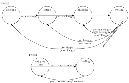
Figure 1.1 visualizes the student’s and one friend’s behavior as a directed graph. Each circle is a local state denoted with a name in the upper half. Edges represent transitions from the parent state to its successor. If a precondition for a transition exists it is given the prefix pre: above the corresponding edge. Postconditions are described under the edges and prefixed with apost:. There is one global variable called completeness denoting thecompletenessof the work not visualized in the graph.
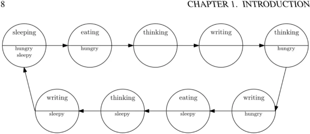
The state space of the student, depicted in Figure 1.2 shows a directed graph of all reachable states for the student, if no interaction with a friend appears. The name of the state is shown in the upper half, and the variables beingtrue in a state are visualized in the bottom half of the circle. In contrast to Figure 1.1 states with similar names appear several times in the state space since the values of the variables in it differ. Figure 1.2 visualizes only the state space of the student omitting interventions of friends. A state space involving correction cycles is a cross product of the state spaces of all actors. So in each state the student is in the friend can be in anenjoying timeor in acorrectingstate, increasing the number of states by a factor of two for each extra friend. Additionally, tracking the completeness variable in the state, e. g., as an integer value between0 and100% would theoretically blow up the state space by a factor of100making reduction and compression strategies essential.
1.2. STATE SPACE EXPLORATION 7
sleeping eating thinking writing
post:not sleepy post:not hungry
pre: not sleepy pre: not hungry
post: hungry pre: hungry post: sleepy pre: sleepy enjoying time reading
post: decreasecompleteness
pre: completeness>0 post: increase completeness Student Friend post: hungry
Figure 1.1: Visualization of the thesis problem as a graph. Circles denote a local state the actor can be in. Each local state is denoted with a name in the upper half of the circle. Edges represent transitions from the parent to the successor with preconditions above it prefixed bypre: and postconditions bypost:. The upper graph presents the transitions for the student and the lower one those for a friend.
Both examples sketch the roots of the states space explosion problem in a simpli-fied manner and motivate the necessity for efficient state storage and processing strate-gies. While a naive implementation of thecompletenessvariable would increase the state space by a factor of 100 the binary representation can reduce the factor to
log(100) = 7. Additional reduction techniques are abstraction (Edelkamp and Lluch-Lafuente, 2004; Namjoshi and Kurshan, 2000) and compression (Lluch-Lafuenteet al., 2002; Clarkeet al., 1994; Korf, 2008b; Holzmann and Puri, 1999).
1.2.3
State Spaces in the Following Parts
Although the following domains seem to be very different the strategy of state space exploration is the connecting aspect. Model checking, Action Planning, Game Solv-ing and Probabilistic Model CheckSolv-ing are all search problems and easily mapped to a graph algorithm. The proposed technique to use recently developed hardware in graph searching is the roof standing on four pillars, depicted in the four disciplines. The next sections will sketch the mapping of each part to graph searching while a detailed mapping is given in each corresponding part.
sleeping hungry
sleepy
eating hungry
thinking writing thinking
hungry writing hungry eating sleepy thinking sleepy writing sleepy
Figure 1.2: The state space containing9states the actorstudentdefined in the thesis problem can be in. The communication with friends, who correct the thesis, is avoided due to complexity of the visualization. When an additional actor (e. g., friend) is in-cluded each state is extended by a local state of the actor increasing the number of states by a factor corresponding to the number of local states the actor can be in. This simplification also abstracts from the completionvariable in the states which would increase the number of states by a factor of100if used as a percent variable.
Model Checking
InModel Checkinga model, describing a system and given in a description language
is checked for a given property. Here, the system is defined prior to the search, given variables and processes as transformable elements, followed by transition functions denoted as transitions. Although the environment is not given explicitly it is given by the model checker who is handling the description language. The goal of finding states violating the property is achieved by checking each single state reachable from an initial state against it. To check lifeness properties a so calledlassopath has to be found. Such a path consists of a cycle containing at least one special (in this discipline denoted asactive) state and that must be reachable from the initial state and defined in the model description. For such a search, special graph traversal algorithms were developed and Part II will propose an extended algorithm. It uses a number of standard graph search algorithms to find the shortest lasso in a state space. The following chapter proposes an approach to efficiently utilize graphics cards when generating the state space in Model Checking.
Action Planning
Action Planning is a scientific domain for finding a plan in a given environment to
achieve a defined goal. The system of Action Planning is an environment for an actor, e. g., a robot. The actor has to perform actions to find a sequence of actions, called plan, to put himself, into a given goal configuration. This plan can be mapped to a path in a graph, starting at an initial state and connecting it to a state where the goal is achieved. The initial state is defined prior to the search and transitions are given by actions in a description language. The way to find such a plan is to generate all states until the goal state is reached and then either search backwards to the initial state, for a plan
1.3. GRAPH SEARCH ALGORITHMS 9
reconstruction, or store the plan while searching. Refined Action Planning usescosts
which map each action to a value to generate a more realistic representation. Here, an exploration considering only the length of a path is not efficient and special graph algorithms (e. g., Dijkstra’s Algorithm (Dijkstra, 1959)), are used. Part III presents a graphics card algorithm extended to support action costs and external media for a generation of the plan.
Game Solving
The system of a game inGame Solvingis the state of the game at a specific stage. In board games it suffices to represent the board and the positions of all pieces on it in the system. The transitions are the rules of the game given prior to the search. The task to decide whether a given player can win the game at a given state is achieved by visiting every state and checking for a path to a winning state. One approach to solve a game is a two searches strategy. In the firstforwardsearch all states reachable from the initial state are generated and classified whether they are winning states for a player or not. The secondbackwardssearch starts at all winning states and propagates the information which player has won to the predecessors. In games with only one winning state, like one player combinatorial games, a forward search from the current state suffices to determine if the game can still be completed. In two player games all terminating winning states have to be identified by a forward search followed by a backward search from these to classify all states up to the initial state. Part IV proposes to compress each state to a number by using a permutation rank strategy or binomial and multinomial hashing to decompress the state on the graphics card and analyze it. This strategy can be evaluated efficiently due to the highly parallel processing power of this unit.
Probabilistic Model Checking
Probabilistic Model Checkingavoids the preconditions of the state space search by
re-placing them with the probability of being active. The probabilities of all preconditions in one state sum up to 100%. On leafs this is achieved by adding an outgoing transi-tion without postconditransi-tions having a probability of 100%. A naive graph theoretical approach to determine the probability of a property violation is to find a path from the initial state to a violating one and compute the probability along it. This approach can be very ineffective in terms of computation time and usually a different technique is used. The state space is mapped to a matrix with the probabilities given in that ma-trix and the probability is computed by solving a set of linear computations using a matrix-vector multiplication approach. Part V decreases the time to find a solution significantly by porting the solving process partially to the graphics card.
1.3
Graph Search Algorithms
Moving from node to node in a graph, respectively traversing a state space, requires a strategy, including a storage- and a decision-rule for the order the successors are
generated in. This section will develop a basic algorithm and extend it to more sophis-ticated strategies optimizing it for different conditions like generating speed or search direction. The development starts with ablind search, not using information about the preferred transitions, and resorts to some form of cost-first shortest path path explo-ration, which requires costs assigned to the edges given in the graph description. Since state spaces can become arbitrarily large the section also introduces algorithms for
ex-ternal search, which utilizes external media like hard disks to store information, and
parallel searchutilizing parallel hardware.
1.3.1
Blind Search
In blind search the order of state expansions is defined by the search algorithm, in-formation about preferred transitions is omitted. While generating a state in a search algorithm the generated successors have to be stored for a potential expansion in the further traversal in a dedicated structure calledopen list.
Definition 13 (Open list) The set of generated, but unexpanded states is called an
Openlist (or justOpen) also denoted as aworking set.
Using only anOpenlist one can already form an algorithm which iscomplete, so it will visit all states in the given state space provided it is circle free.
Algorithm 1.1:Graph algorithm using anOpenlist Input:sˆ∈ Sinitial state,Tset of transitions
1 Open←sˆ; {storeˆsinOpen}
2 whileOpen6=∅do {repeat until search terminates} 3 choose a states∈Open; {usually the first one in the list} 4 expand successorss→s1. . . sν; {apply transitions to generate successors} 5 forsi(∀i: 1≤i≤ν)do {check each successor} 6 ifsi∈/ Openthen {when not already inOpen}
7 Open←si; {add it toOpen}
8 removesfromOpen; {all successors generated so state can be dropped}
After inserting the initial state into theOpenlist, Algorithm 1.1 generates the suc-cessors of a state by checking the preconditions and applying corresponding postcon-ditions and stores them in Open. When all successors of a state are generated and inserted intoOpenthe state is removed from the list.
Lemma 2 Algorithm 1.1 will terminate and expand all paths in the state space, visiting all states, if the state space is cycle free.
Proof. Each state remains inOpenuntil all its successors are generated. Removing a fully expanded state is safe since all paths crossing this state to its successors are extended by at least one state. Leaves, states without successors, are end points of paths which cannot be extended and are removed fromOpenimmediately when generated.
1.3. GRAPH SEARCH ALGORITHMS 11
Since the state space is cycle free each path fromˆshas to end with a leaf forcing
the algorithm to terminate.
For state spaces containing cycles Algorithm 1.1 has to be extended. Consider a transition setT with two transitions{(ˆs, s),(s,ˆs)}from the initial state to a successor and back to the initial state. The algorithm will add the initial state toOpenover and over again, being trapped in the cycle unable to terminate. To avoid this behavior an option is needed to decide whether a duplicate of a state was already removed from
Open, thus the states removed fromOpenare stored in a separate structure.
Definition 14 (Closed list) When all successors of a state are generated it is moved to theClosedlist (usually justClosed), also denoted asvisited set.
Algorithm 1.2:Graph algorithm using anOpenand aClosedlist Input :sˆ∈ Sinitial state,Tset of transitions
1 Open←sˆ; {storesˆinOpen}
2 Closed← ∅; {clearClosedlist}
3 whileOpen6=∅do {repeat until search terminates} 4 choose a states∈Open; {usually the first one in the list} 5 expand successorss→s1. . . sν;{apply transitions to generate successors} 6 forsi(∀i: 1≤i≤ν)do {check each successor} 7 ifsi∈/ Open∧si∈/Closedthen {when not already expanded}
8 Open←si; {add it toOpen}
9 removesfromOpen; {all successors generated, so state can be removed}
10 Closed←s; {addstoClosed}
Algorithm 1.2, which extends Algorithm 1.1 by aClosed list, detects duplicates using the lines6to8and avoids adding them to theOpenlist.
Lemma 3 Algorithm 1.2 will terminate and expand all states reachable in the state space, visiting each state exactly once.
Proof. For state spaces without cycles the duplicate detection is not needed, here the proof of Algorithm 1.1 can be applied.
Let us assume a cycle exists and statesc is the first reached state on this cycle.
Line 8 ensures that sc is stored in Open on the first appearance and line10 stores
it in Closed when it has been expanded. While extending all paths crossingsc the
algorithm will reach it again, but avoid inserting it into Open since it was already inserted or expanded. When a duplicate ofsc exists it will also be bypassed which
does not matter since the states behind this duplicate also exist behindsc.
In the example given above, with transitions{ˆs, s),(s,sˆ)}, Algorithm 1.2 will not addˆsa second time toOpensince it is already present inClosed. Although the pseu-docode is extended only in two lines the problem of looking up a state in theClosed
1 2 3 4 5 6 7 10 11 12 13 14 15 8 9 16 Figure 1.3: BFS ordering of states.
1 2 8 11 3 6 9 4 5 7 10 13 15 12 14 16 Figure 1.4: DFS ordering of states.
list should not be underestimated. Many strategies exist and scientists are still develop-ing new ways to either perform or avoid a random lookup, or storeClosedefficiently on external media without the necessity to perform a scan through the complete file for each generated state. Based on Algorithm 1.2 several strategies were developed to traverse state spaces efficiently, and this work is another contribution to these strategies. The most prominent algorithms are Breadth-First search (BFS) andDepth-First
search(DFS) (Knuth, 1973). The difference between those algorithms is only the order
of storing states inOpen. BFS stores them in a First In / First Out strategy while DFS uses a Last In / First OutOpenstructure.
Algorithm 1.3:Breadth-First search
Input :ˆs∈ Sinitial state,T set of transitions
1 Open←sˆ; {storeˆsinOpen}
2 Closed← ∅; {clearClosedlist}
3 whileOpen6=∅do {repeat until search terminates} 4 choosefirststates∈Open;
5 expand successorss→s1. . . sν; {apply transitions to generate successors} 6 forall thesi(∀i: 1≤i≤ν)do {check each successor} 7 ifsi∈/ Open∧si ∈/ Closedthen {when not already expanded}
8 Open←si; {add it to theendofOpen}
9 removesfromOpen; {all successors generated so state can be removed}
10 Closed←s; {addstoClosed}
Algorithm 1.3 visits all states ordered by the distance to ˆswhile Algorithm 1.4 visits states with a maximal distance toˆsfirst. In contrast to Algorithm 1.2 the order of storing states in theOpenlist is given explicitly by the algorithm.
Since only the order of storing the states inOpenis different to the general algo-rithm the proof of completeness is inherited from the previous algoalgo-rithms. The differ-ence in the order of visiting nodes is displayed in Figures 1.3 and 1.4.
Algorithm 1.3 partitionsS into BFS-Layers. All states in a BFS-Layer have the same distance from the initial state.
1.3. GRAPH SEARCH ALGORITHMS 13
Algorithm 1.4:Depth-First search
Input :sˆ∈ Sinitial state,Tset of transitions
1 Open←sˆ; {storesˆinOpen}
2 Closed← ∅; {clearClosedlist}
3 whileOpen6=∅do {repeat until search terminates} 4 choosefirststates∈Open;
5 expand successorss→s1. . . sν;{apply transitions to generate successors} 6 forall thesi(∀i: 1≤i≤ν)do {check each successor} 7 ifsi∈/ Open∧si∈/Closedthen {when not already expanded} 8 Open←si; {add it to thebeginningofOpen} 9 removesfromOpen; {all successors generated so state can be removed}
10 Closed←s; {addstoClosed}
Table 1.1: Main differences between BFS and DFS.
BFS DFS
speed slow fast
Opensize bound by largest layer bound by depth cycle detection none by checking new states inOpen
distance to initial minimal not specified
Although the difference in pseudocode is marginal the impact on the evaluation of the algorithm is not. Table 1.1 points out some of the main differences. The DFS algorithm turns out to be much faster on today’s hardware due to its better cache effi-ciency. Although the work to expand all states is the same the BFS algorithm stores a large number of states in memory and fetches a state from a distant region of it for expansion. In contrast DFS expands the last generated state which resides often still in the cache of the CPU. On the other hand the BFS algorithm can be parallelized trivially by sending generated successors to different nodes. For the DFS algorithm an efficient parallelization is much harder to realize since only one successor of a parent is gen-erated. Memory consumption ofOpenalso differs significantly in both approaches, while in BFS the next BFS-Layer has to be stored inOpenDFS stores the path from the initial state to the current one. This path is especially short in state spaces with a low BFS-depth but a high branching factor. Storing the entire path from initial also enables a trivial cycle detection extension to the algorithm. By simply checking each generated state for a duplicate inOpenall cycles reachable fromsˆare found. In BFS this strategy fails due to all states inOpenhaving the same distance to the initial. How-ever, in BFS this distance is guaranteed to be minimal while in DFS the depth at which a state is found depends highly on the state space and the chosen successor to generate. To connect the optimality in depth and the speed of single expansions Korf (1985) presentediterative deepening(Korf, 1985) as described in Algorithm 1.5. Here a DFS is started with a maximal depthmaxdgiven before the search. When the desired goal
Algorithm 1.5:Iterated Depth-First search Input :ˆs∈ Sinitial state,T set of transitions Output: minimal path to goal state if it exists
1 Open←sˆ; {storeˆsinOpen}
2 Closed← ∅; {clearClosedlist}
3 maxd←2; {depth bound for first iteration} 4 whileiteratedo {repeat until whole state space generated} 5 iterate←false; {variable to force another iteration} 6 whileOpen6=∅do {repeat until search terminates} 7 choosefirststates∈Open;
8 expand successorss→s1. . . sν; {apply transitions to generate successors}
9 forall thesi(∀i: 1≤i≤ν)do {check each successor} 10 ifsi∈/ Open∧si ∈/ Closedthen {when not already expanded} 11 if|Open|+ 1> maxdthen {states exist under the bound}
12 iterate←true
13 else
14 Open←si; {addsito thebeginningofOpen} 15 ifsi∈goalthen returnOpen; {return path to goal} 16 removesfromOpen;
{all successors generated so state can be removed}
17 Closed←s; {addstoClosed}
18 maxd←maxd+ 1; {increase depth bound}
state is not found the depth bound is increased and the search restarted. When no length of a path exceeds the bound the search terminates. This algorithm is not complete, it does not necessarily expand all states up to the given search border.2 Although a DFS
is used, the path delivered to the goal is minimal due to the increasing border by one and a goal is reported at the minimal depth bound.
All blind algorithms assume that transitions are preferred according to the given expansion strategy. When the state space description includes an ordering on the tran-sitions the algorithm has to take this into account while expanding. One possibility used in planning to impose an ordering on transitions is assigning themcostsof evalu-ation by defining acost function.
Definition 15 (Cost Function) Acost functioncost is a mappingT → Rassigning
eacht∈T a cost value.
2Assume a search border ofbfor a given iteration and a statesin a depthbthenscan be reached by
the search and stored inClosed. When reached again in a lower depth it will not be expanded due to its existence inClosedand its successors will be omitted.
1.3. GRAPH SEARCH ALGORITHMS 15
Analogously the cost of a path is defined as follows.
Definition 16 (Cost of a Path) Thecostcost(s0. . . sn) for a given path(s0. . . sn)is the sum of all costs of transitions applied in the path
n−1 X
i=0
cost(t(si, si+1))
.
In state spaces with uniform costs, e. g.,cost(t) =c∀t ∈T, the length of a path conforms tocost(s0, . . . , sn−1)/c.
Given a cost function, and interested in the path with minimal costs, Dijkstra pre-sented a graph traversal algorithm in 1959 expanding nodes in the order of increasing costs. Algorithm 1.6 applicable to state spaces stores pairs (s,cost(s))inOpen or-dered bycost()to compute the summarized costs for a path.
Algorithm 1.6:Dijkstra’s Algorithm
Input:sˆ∈ Sinitial state,Tset of transitions,cost:T →Rtransitions to costs
mapping
Output:pathcost: minimal costs for each state reached on a path fromsˆ
1 Open←(ˆs,0); {storesˆandcost(ˆs) inOpen}
2 Closed← ∅; {clearClosedlist}
3 whileOpen6=∅do {repeat until search terminates} 4 choose the states∈Openwith minimal costs ; {e. g., in a priority queue} 5 expand successorss→s1. . . sν;{apply transitions to generate successors} 6 forall thesi(∀i: 1≤i≤ν)do {check each successor} 7 ifsi∈/ Closedthen {look intoOpenANDClosed} 8 Open←(si,cost(si)); {storestateiandcost(si)inOpen}
9 else
10 ifsi∈Openandcost(si)<cost(duplicate inOpen)then
11 cost(duplicate inOpen)←cost(si); {update the cost inOpen}
12 removesfromOpen; {all successors generated so state can be removed} 13 pathcost←(s,cost(s)); {storesandcost(s)to return it}
14 Closed←s; {addstoClosed}
15 returnpathcost;
Algorithm 1.6 looks inClosedfor duplicates but also checks for existence of the state inOpenwhich is mandatory to update the costs for already generated but still not expanded states which were reached again using a cheaper path. To maintain Open
sorted priority queues (Edelkamp and Wegener, 2000; Cormenet al., 2001) are used to speed up the algorithm.
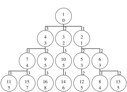
Table 1.2: Dijkstra ordering of nodes inClosed. The position is given in the upper array and the path cost in the lower. The nodes are expanded in the order of their path costs.
Position 1 2 3 4 5 6 7 8 9 . . . 13 14 15 16 Path costs 0 1 2 3 3 3 4 4 5 . . . 5 6 7 8
Lemma 4 Algorithm 1.6 returns the minimal cost of a path for all states reachable from the initial one for state spaces with non-negative costs.
Proof. The algorithm partitions the state space in layers of equal costs. First consider state spaces with uniform costscost(t) = c(∀t ∈T). Here the algorithm partitions the state space according to the BFS-Layers since the path costs start with0 at the initial state and increase bycwith every added state.Openis always strictly sorted by the costs and every new state is added at the end having costs equal or higher to the previous one
• if a statesiis a successor ofsits costs arecost(ˆs, si) =cost(ˆs, s) +c.
• if two statessi andsj are successors of a states, the costs arecost(ˆs, si) = cost(ˆs, sj) =cost(ˆs, s) +c.
In state spaces with non-uniform and non-negative costscost(t) =c≥0 (∀t∈T) the state space is partitioned in layers of equal costs. Assume we sortOpenafter each insertion. With non-negative costs we havecost(ˆs, si ∈ Succ(s))≥ cost(ˆs, s), and
when a stateso ∈Openis being expanded the costs to reach itcost(ˆs, so)is minimal
compared to all remaining states inOpen. So each new generated statesi ∈Succ(s)
is sorted behindsand an update of its cost can move it only further to the front of
Openbut not befores. Whensis expanded its costs will never again be updated since for all statesso ∈Openwe havecost(ˆs, s)≤cost(ˆs, so)so all remaining states will
be added toClosed, and topathcostin a non-decreasing order of costs. After adding a cost function to the state space given in Figures 1.3 and 1.4 with costs in the range of1. . .3the Dijkstra algorithm is applied, resulting in a state ordering given in Figure 1.5. The states contain the expansion order at the top and the path cost at the bottom of a state depicted by a circle. Table 1.2 depicts the numbers again to visualize the implied ordering by path cost.
1.3.2
External Search
State space traversal algorithms consume a huge amount of memory. Storing all states of an implicitly given graph in RAM can be impossible given on the size of the graph. Solving the problem by using compression is a solution, but even with compression a minimal size for a state exists limiting the amount of states which can be stored.
Another approach is to store the nodes on external memory e. g., a HDD. Since hard disk drive has different access properties then internal memory, new algorithms had to be developed to utilize it efficiently.
1.3. GRAPH SEARCH ALGORITHMS 17 4 3 2 7 9 10 11 15 16 14 12 8 5 6 13 1 2 3 3 3 3 1 1 1 1 2 2 2 2 2 1 2 3 0 1 3 6 5 4 5 5 7 8 4 5 5 3
Figure 1.5: Dijkstra ordering of states in a virtual state space. The expansion order is given in the upper half, the path cost in the lower half of each circle. Edges are marked with the edge costs.
Data is stored in blocks on external media imposing a lag when accessing a random block or a single element in this block. Adjacent blocks of memory can be accessed without a latency, so accessing data is done sequentially since this strategy distributes the latency on all retrieved elements. Aggarwal and Vitter invented an adapted mem-ory model to analyze algorithms that utilize external memmem-ory in 1988. Here accessing the data in blocks is preferred to analyze the performance of external memory algo-rithms. Graph traversal algorithms optimized for external memory usage are presented in (Meyeret al., 2003).
Algorithm 1.7:The External BFS algorithm
Input :sˆ∈ Sinitial state,Tset of transitions,bufferpreferably size of RAM
1 Open←sˆ; {storesˆinOpen}
2 whileOpennot emptydo
3 readOpeninbuffer; {partially if to large}
4 expand all states inbufferinto a new fileOpennexton external device ;
5 sortOpennext; {externally if necessary}
6 scan throughOpennextand remove adjacent duplicates ;
7 scan troughOpenandOpennextto remove duplicates from previous layers ; 8 appendOpennexttoOpen;
Algorithm 1.7 presents a Breadth-First search approach (Munagala and Ranade, 1999), where all data is stored on external media. Internal memory is used as abuffer
where nodes are stored temporarily before being written to the block device. Enabling an efficient duplicate detection is realized by sorting. Since theOpennextfile,
contain-ing all states to be expanded in the next BFS-Layer can potentially exceed the available buffer size an external sorting approach is needed. Being sorted, all duplicates in the file will be arranged adjacent to each other and can be removed easily by a single scan through the file. Mehlhorn and Meyer (2002) and later on Ajwaniet al.(2007) present modifications of this algorithms with a reduced number of I/O operations due to caching an adjacency matrix of the nodes in the internal memory, reducing the running time by several folds.
While the presented modifications request an explicitly given graphs Korf (2003a) presents an implicit graph algorithm based on the idea of aFrontier Searchanalyzed in detail also by Korf in 2005.
Since the efficiency of an external algorithm highly depends on its implementation two C++ libraries exist to support the developer. Thestandard template library for XXL
data sets(STXXL) (Dementievet al., 2005), used in the scope of this work, is the first
I/O-efficient algorithm library that supports the pipelining technique. While the goal of theTemplated Parallel I/O Environment(TPIE) is to provide a portable, extensible, flexible, and easy to use C++ programming environment.
1.3.3
Parallel Graph Search
Parallel graph search (an overview is given e. g., by Ghosh (1993)) increases the search-ing speed by utilizsearch-ing more then one computation device to generate states or to check for duplicates and extends the available internal memory by using a distributed system. The challenge in parallel search is to find distinct parts of a graph and to distribute them to the computation cores.
Parallel search is divided in two sub domains calleddistributed searchandshared
memory search. Distributed search denotes the utilization of clusters, build up of a
number of distinct computing systems connected through a network. Shared memory search relays on the existence of a memory accessible directly from all used computa-tion devices.
Distributing a state space is usually done in one of two ways, either a static hash like function is used to determine which core is responsible for the state or a dynamic function analyzes the load on the cores and assigns a generated successor to a core with the minimal load. Both strategies are divided into further solutions to optimize the distribution and minimize the necessary communication.
A naive approach to parallelize the Breadth-First search (Ghosh and Bhattacharjee, 1984), depicted in Algorithm 1.8 is to distribute the generated successors among the available computing nodes. The problem with this realization is a high communication overhead between the nodes. Each generated state is send over a communication proto-col to a distant node and a commonClosedstructure has to be maintained to avoid the expansion of duplicates. Additionally to aClosedsynchronization theOpenstructure of this algorithm has to be maintained on arootnode.
The modified Algorithm 1.9 utilizes a hash function h(s) to distribute states to indexed nodes enabling a distribution ofClosedandOpenstructure. Thishash based
partitioningavoids the communication to determine already visited states but depends
1.3. GRAPH SEARCH ALGORITHMS 19
Algorithm 1.8:Basic parallel search strategy Input :sˆ∈ Sinitial state,Tset of transitions
1 Open←sˆ; {storesˆinOpen}
2 Closed← ∅; {clearClosedlist}
3 whileOpen6=∅do {repeat until search terminates} 4 choosenstatessp∈Open;
5 forall thesp(∀p: 0≤p≤n−1)do in parallel 6 expand successorssp→s1. . . sν;
{apply transitions to generate successors}
7 forall thesi(∀i: 1≤i≤ν)do {check each successor} 8 ifsi∈/ Closedthen {when not already expanded}
9 Open←si; {add it toOpen}
10 remove allspfromOpen;
{all successors generated so states can be removed}
11 Closed←s; {addstoClosed}
Algorithm 1.9:Hash based parallel search strategy
Input :sˆ∈ Sinitial state,Tset of transitions,Nnumber of nodes
1 Open[0]←sˆ; {storeˆsinOpenof one node} 2 forall the nodesn(0≤n < N)do in parallel {start all nodes} 3 Closed[n]← ∅; {clear localClosedlist} 4 whileOpen[0, . . . , N −1]6=∅do {repeat until allOpenempty} 5 choose one states∈Open[n];
6 ifs /∈Closed[n]then {when not already expanded} 7 expand successorss→s1. . . sν;
{apply transitions to generate successors}
8 forall thesi(∀i: 1≤i≤ν)do {check each successor} 9 ifh(si)6=nthen {find responsible node for this state} 10 sendsito nodeh(si); {send it to appropriate state}
11 else
12 Open[n]←si; {add it to localOpen}
13 removesfromOpen[n];
{all successors generated so state can be removed}
Node 0 Node 1
Node 2 Node 0
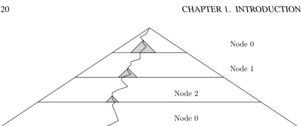
Figure 1.6: Distribution of nodes according to the DFS distance to the initial like pro-posed by (Holzmann and Bosnacki, 2007).
Zhou and Hansen (2007) presented a structured based parallel distributing approach which analyzes the state space prior to the search and distributes the states based on a state space abstraction function. Here, the advantage is the preferred expansion of successors on the same node, so each node can work on a specific region in the state space and distribute only distant states. They extended this strategy to a dynamic dis-tribution technique. Here the state space is analyzed on the fly while searching and the distribution function adjusted (Zhou and Hansen, 2011). An adjustment includes a stop of the search and a rearrangement of already stored states.
While the previous parallelizations are based on BFS and can be used on shared memory and distributed systems, (Holzmann and Bosnacki, 2007) went a different ap-proach and parallelized the Depth-First search on a shared memory multi-core system. Here, the states are distributed among the available cores depending on their DFS dis-tance from the initial state like sketched in Figure 1.6. When all nodes are occupied the search continues on the first node which preferably expands states at a higher depth.
Recently Barnatet al.(2011) show how existing parallel algorithms to find strongly connected components in a graph can be reformulated in order to be accelerated by NVIDIA CUDA technology. In particular, they design a new CUDA-aware proce-dure for pivot selection and adapt selected parallel algorithms for CUDA accelerated computation.
DisNet, a tool set for Distributed Graph Computation (Lichtenwalter and Chawla, 2011) should be given as the latest example for a distributed graph search implemen-tation. After supplying two small fragments of code describing the fundamental kernel of the computation. The framework automatically divides and distributes the workload and manages completion using an arbitrary number of heterogeneous computational resources.
Describing all possible ways to parallelize a state space search is sincerely out of the scope of this introduction and even not possible due to the large number. The sketch, given in this section is mentioned as a starting point for the following assumptions and development leading to an efficient algorithm for novel hardware.
1.4. DUPLICATE DETECTION IN GRAPH SEARCH 21
1.4
Duplicate Detection in Graph Search
All state space searching algorithms rely on an efficient duplicate detection. In fact studies made within the scope of this work revealed the duplicate detection to consume over 50% of the whole searching time. So several strategies were developed to avoid re-expanding nodes. Removing already existing nodes requires a comparison function for state representations. This function can either compare the complete stored vectors or an approximated representation of them giving the chance to reduce the space needed to represent the state.
The challenge in duplicate detection is to find an already expanded state which is similar to the examined one, done either by sorting the new state into all existing ones or by looking up an entry in a table containing expanded states. While the sorting method is superior on block access devices with a slow random access, looking up an entry table is superior in memory structures with a short random access speed. Variations exist to speed up the checking process by either reducing the number of comparisons or the amount of memory used for the expanded states.
In special cases, where enough information of the state space is given prior to the search it is possible to reduce the duplicate detection to only special states or even avoid it completely. In his thesis Jabbar (2008) has shown that when exploring undirected graphs with the BFS algorithm a check of the previous two layers suffices to remove all duplicates.
External search introduces the termDelayed Duplicate Detection(DDD) in con-trast toImmediate Duplicate Detection(IDD) defined as follows.
Definition 17 (Delayed/Immediate Duplicate Detection) In Delayed Duplicate De-tection (Korf, 2003a) the detection of duplicates is postponed to a specific point in the search, e. g., when one BFS-Layer is generated, to increase per state performance. Taking into account that states may be stored more then once.
Immediate Duplicate Detectionchecks for existing duplicates immediately after a new state is generated, avoiding memorizing of duplicates.
1.4.1
Hash Based Duplicate Detection
To achieve a fast duplicate detection, also facing the rising amount of RAM available in today’s systems hashing can be used.
Definition 18 (Hash Function) Ahash functionhis a mapping of some universeUto an index set[0, . . . , m−1].
The set of reachable statesS is a subset ofU, i. e.,S ⊆ U. SinceS is usually not known prior to the search, the hash functionhis defined over all elements in the universe. The upper bound form−1is the number representation in the system being 2b whereb is the number of bits used to store the value. A generated statesor its
representation is stored at a specific position in a table. Usually the predefined position for sish(s) modtablesize wheretablesizeis the maximal number of elements the table can host.