Integrated Feature and Parameter Optimization for an
Evolving Spiking Neural Network
Stefan Schliebs, Micha¨el Defoin Platel, and Nikola Kasabov Knowledge Engineering and Discovery Research Institute,
Auckland University of Technology, New Zealand
{sschlieb,nkasabov}@aut.ac.nz
Department of Computer Science, University of Auckland
Abstract. This study extends the recently proposed Evolving Spiking Neural Network (ESNN) architecture by combining it with an optimization algorithm, namely the Versatile Quantum-inspired Evolutionary Algorithm (vQEA). Follow-ing the wrapper approach, the method is used to identify relevant feature subsets and simultaneously evolve an optimal ESNN parameter setting. Applied to care-fully designed benchmark data, containing irrelevant and redundant features of varying information quality, the ESNN-based feature selection procedure lead to excellent classification results and an accurate detection of relevant information in the dataset. Redundant and irrelevant features were rejected successively and in the order of the degree of information they contained.
1
Introduction
In many recent studies attempts have been made to use Spiking Neural Networks (SNN) for solving practical real world problems. It was argued that SNN have at least similar computational power than the traditional Multi-Layer-Perceptron derivates [1]. Sub-stantial progress has been made in areas like speech recognition [2], learning rules [3] and associative memory [4]. In [5] an evolving SNN (ESNN) was introduced and ap-plied to pattern recognition problems, later this work was extended to speaker authenti-cation tasks and even to audio-visual pattern recognition [10]. A similar spiking neural model was analyzed [7], in which a classification problem for taste recognition was addressed. Based on a simple but efficient neural model, these approaches used the ESNN architecture, which was trained by a fast one-pass learning algorithm. Due to its evolving nature the model can be updated whenever new data becomes available, with-out requiring the re-training of earlier presented data samples. Some promising results could be obtained both on synthetic benchmark and real world datasets.
This study investigates the potential of ESNN when applied to Feature Subset Se-lection (FSS) problems. Following the wrapper approach the ESNN architecture com-bined with an evolutionary algorithm. The latter one is used to identify relevant feature subsets and simultaneously evolve an optimal parameter setting for the ESNN, while the ESNN itself operates as a quality measure for a presented feature subset. By opti-mizing two search spaces in parallel it is expected to evolve an ESNN configuration, specifically generated for the given dataset and a specific feature subset, that maximizes classification accuracy.
Algorithm 1 Training an Evolving Spiking Neural Network (ESNN) Require: ml∈(0,1), sl∈(0,1), cl∈(0,1), l∈L
1: initialize neuron repositoryRl={} 2: for all samplesX(i)belonging to classldo
3: w(ji)←(ml)order(j), ∀j|jpre-synaptic neuron of i 4: P SPmax(i) ← P jw (i) j (ml)order(j) 5: θ(i)←c lP SP( i) max 6: if min(d(w(i), w(n)))> s l, w(n)∈Rl then 7: w(n)←mergew(i)andw(n) 8: θ(n)← mergeθ(i) andθ(n) 9: else 10: Rl←Rl∪ {w(i)} 11: end if 12: end for
2
ESNN Architecture for FSS
The ESNN architecture uses a computationally very simple and efficient neural model, in which early spikes, received by a neuron, are stronger weighted than later ones. The model was inspired by the neural processing of the human eye, which performs a very fast image processing. Experiments have shown that a primate only needs several hun-dreds of milliseconds to make reliable decisions about images that were presented in a test scenario [8]. Since it is known that neural image recognition involves several suc-ceeding layers of neurons, these experiments suggested that only very few spikes could be involved in the neural chain of image processing. In [9] a mathematical definition of these neurons was attempted and tested on some face recognition tasks, reporting encouraging experimental results. The same model was later used by [10, 6] to perform audio-visual face recognition.
Similar to other SNN approaches a specific neural model, a learning method, a network architecture and an encoding from real values into spike trains needs to be defined in the ESNN method. The neural model is given by the dynamics of the post-synaptic potential (PSP) of a neuroni:
P SPi(t) =
0 if neuron has fired
P
j|f(j)<twji×(mi)order(j) else (1) where wji is the weight of a pre-synaptic neuron j, f(j)the firing time of j, and
mi∈(0,1)a parameter of the model, namely the modulation factor. Functionorder(j) represents the rank of the spike emitted by neuronj. For example a rankorder(j) = 0 would be assigned, if neuronj is the first among all pre-synaptic neurons that emits a spike. In a similar fashion the spikes of all pre-synaptic neurons are ranked and then used in the computation ofP SPi. A neuronifires a spike when its potential has reached a certain thresholdθ. After emitting a spike the potential is reset toP SPi = 0. Each neuron is allowed to emit only a single spike at most. The thresholdθ=c P SPmaxis set to a fractionc∈(0,1)of the maximal potentialP SPmaxpossible by a neuron.
-2 -1 0 1 2 0.0 0.2 0.4 0.6 0.8 1.0 Excitation 0 1 Neuron2 3 4 0.0 0.2 0.4 0.6 0.8 1.0
Firing Time Receptive FieldsInput Value (a) Stimulus Spikes 0 2 Time in sec4 6 8 0.0 0.2 0.4 0.60.8 1.0 PSP (b)
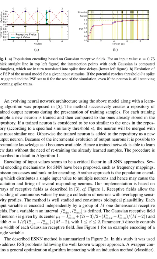
Fig. 1. a) Population encoding based on Gaussian receptive fields. For an input valuev= 0.75
(thick straight line in top left figure) the intersection points with each Gaussian is computed (triangles), which are in turn translated into spike time delays (lower left figure). b) Evolution of the PSP of the neural model for a given input stimulus. If the potential reaches thresholdθa spike is triggered and the PSP set to 0 for the rest of the simulation, even if the neuron is still receiving incoming spike trains.
An evolving neural network architecture using the above model along with a learn-ing algorithm was proposed in [5]. The method successively creates a repository of trained output neurons during the presentation of training samples. For each training sample a new neuron is trained and then compared to the ones already stored in the repository. If a trained neuron is considered to be too similar to the ones in the repos-itory (according to a specified similarity thresholds), the neuron will be merged with the most similar one. Otherwise the trained neuron is added to the repository as a new output neuron. Because of the incremental evolution of output neurons it is possible to accumulate knowledge as it becomes available. Hence a trained network is able to learn new data without the need of re-training the already learned samples. The procedure is described in detail in Algorithm 1.
Encoding of input values seems to be a critical factor in all SNN approaches. Sev-eral encoding mechanisms for SNN have been proposed, such as frequency mappings, Poisson processes and rank order encoding. Another approach is the population encod-ing which distributes a sencod-ingle input value to multiple neurons and hence may cause the excitation and firing of several responding neurons. Our implementation is based on arrays of receptive fields as described in [3], cf. Figure 1. Receptive fields allow the encoding of continuous values by using a collection of neurons with overlapping sensi-tivity profiles. The method is well studied and constitutes biological plausibility. Each input variable is encoded independently by a group ofM one dimensional receptive fields. For a variablenan interval[In
min, Imaxn ]is defined. The Gaussian receptive field of neuroniis given by its centerµi =Iminn + (2i−3)/2∗(Imaxn −Iminn )/(M−2))and widthσ= 1/β(In
max−Iminn )/(M−2), with1≤β≤2. Parameterβdirectly controls the width of each Gaussian receptive field. See Figure 1 for an example encoding of a single variable.
The described ESNN method is summarized in Figure 2a. In this study it was used to address FSS problems following the well known wrapper approach. A wrapper con-tains a general optimization algorithm interacting with an induction method (classifier).
(a) (b)
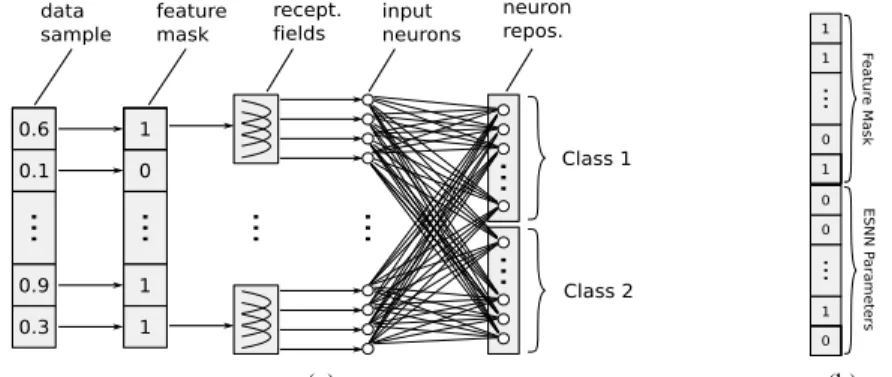
Fig. 2. a) ESNN architecture – A data sample is masked to extract a feature subset, then each variable is translated into trains of spikes. The resulting spike sequence invokes a spiking neural network and a repository of output neurons is successively generated during the training process. b) Chromosome used in vQEA for simultaneously optimizing feature and parameter space.
The optimization task consists in a proper identification of an optimal feature subset, which maximizes the classification accuracy determined by the inductor. The ESNN architecture will operate as the induction method during the course of this paper. Due to its interesting properties in terms of solution quality and convergence speed we de-cided to use the previously proposed Versatile Quantum-inspired Evolutionary Algo-rithm (vQEA) [11] as the optimization algoAlgo-rithm. The method evolves in parallel a number of independent probability vectors, which interact at certain intervals with each other, forming a multi-model Estimation of Distribution Algorithm (EDA) [12]. It has been shown that this approach performs well on epistatic problems, is very robust to noise, and needs only minimal fine-tuning of its parameters. In fact the standard setting for vQEA is suitable for a large range of different problem sizes and classes. Finally vQEA is a binary optimizer and fits well to the feature selection problem we want to apply it on.
Manual fine-tuning the neuronal parameters can quickly become a challenging task [6]. To solve this problem the idea of the simultaneous optimization of the two combi-natorial search problems of FSS and learning of parameters for the induction algorithm was proposed [13]. The selection of the fitness function was identified to be a crucial step for the successful application of such an embedded approach. In the early phase of the optimization the parameter configurations are selected randomly. As a result it is very likely that a setting is selected for which the classifier is unable to respond to any input presented, which corresponds to flat areas in the fitness landscape. Hence a configuration that will allow the network to fire (even if not correctly) represents a huge (local) attractor in the search space, which could be difficult to escape in later iterations of the search. In [13] a linear combination of several sub-criteria was used to avoid a too rugged fitness landscape. Nevertheless we can not confirm, that the use of much sim-pler fitness functions led to any problems in our experiments. Using the classification accuracy on testing samples seemed to work well as it is presented later in this paper. All parameters modulation factorml, similarity thresholdsl, PSP fractioncl,∀l ∈ L
of ESNN were included in the search space of vQEA. Due to its binary nature vQEA requires the conversion of bit strings into real values. We found that a small number of Grey-coded bits were sufficient to approximate meaningful parameter configurations of the ESNN method. In Figure 2b the structure of a chromosome as it is used in vQEA is depicted.
3
Experiments
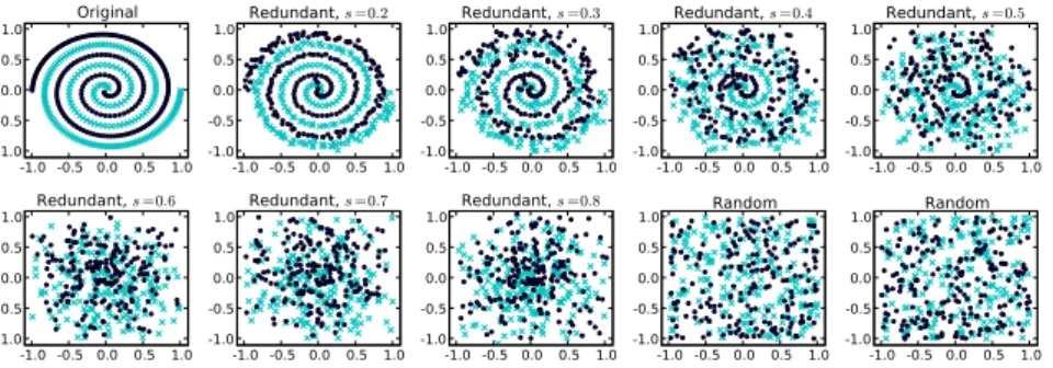
We have applied the vQEA optimised Evolving Spiking Neural Network (ESNN) ar-chitecture on the Two-Spiral problem firstly introduced in [14]. It is composed of two-dimensional data forming two intertwined spirals. It requires the learning of a highly non-linear separation of the input space. The data was frequently used as a benchmark for neural networks, including the analysis of the ESNN method itself [6]. Since the data contains only two relevant dimensions we have extended it by adding redundant and random information. The importance of the redundant features was varied: Fea-tures range from mere copies of the original two spirals to completely random ones. The information available in a feature decreases when stronger noise is applied. The generation of the dataset is particularly interesting, since it is expected that the ESNN is capable of rejecting features according to their inherent information, i.e. , the less information a feature carries, the earlier ESNN should be able to discard the feature during the selection process. We will briefly summarize the data generation below.
Data points belonging to two intertwined Archimedean spirals (also known as the arithmetic spiral) were generated and labelled accordingly. The irrelevant dimensions consist of random values chosen from a uniform distribution, covering the entire input space [−1,1]of the dataset. The redundant dimensions are represented by copies of the original spiral pointsp= (x, y)T, which were disturbed by a Gaussian noise using standard deviationσ = |p| ∗s, with|p|being the absolute value of vectorpandsa parameter controlling the noise strength. The noise increases linearly for points which are more distant from the spiral origin(0,0)T. A noisy valuep′
iis then defined as the outcome of thepi-centered Gaussian distributed random variableN(pi, σ2), usingσas defined above.
Our final dataset contained seven redundant two-dimensional spiral points(x′i, y′i)T, for each a different noise strength parameters∈ {0.2,0.3, . . . ,0.8}was used, totalling in 14 redundant features. Additional four random features r1, . . . , r4 were included. Together with the two relevant features of the spirals (xandy) the dataset contained 20 features. Figure 3 presents the 400 generated samples of the resulting dataset.
For vQEA we chose a population structure of ten individuals organized in a single group, which is globally synchronized every generation. This setting was reported to be generally superior for a number of different benchmark problems [12]. The learning rate was set toθ=π/100and the algorithm was allowed to evolve over a total number of 400 generations. In order to guarantee statistical relevance 30 independent runs were performed, using a different seed for each of them.
Additional to the feature space, vQEA was used to optimize the parameter space of the ESNN architecture. For each classl ∈ Lthree parameters exist: The modulation factorml, the similarity thresholdsl, and the proportion factorcl. Since the data
rep--1.0 -0.5 0.0 0.5 1.0 -1.0 -0.5 0.0 0.5 1.0 Original -1.0 -0.5 0.0 0.5 1.0 -1.0 -0.5 0.0 0.5 1.0 Redundant, s =0.2 -1.0 -0.5 0.0 0.5 1.0 -1.0 -0.5 0.0 0.5 1.0 Redundant, s =0.3 -1.0 -0.5 0.0 0.5 1.0 -1.0 -0.5 0.0 0.5 1.0 Redundant, s =0.4 -1.0 -0.5 0.0 0.5 1.0 -1.0 -0.5 0.0 0.5 1.0 Redundant, s =0.5 -1.0 -0.5 0.0 0.5 1.0 -1.0 -0.5 0.0 0.5 1.0 Redundant, s =0.6 -1.0 -0.5 0.0 0.5 1.0 -1.0 -0.5 0.0 0.5 1.0 Redundant, s =0.7 -1.0 -0.5 0.0 0.5 1.0 -1.0 -0.5 0.0 0.5 1.0 Redundant, s =0.8 -1.0 -0.5 0.0 0.5 1.0 -1.0 -0.5 0.0 0.5 1.0 Random -1.0 -0.5 0.0 0.5 1.0 -1.0 -0.5 0.0 0.5 1.0 Random
Fig. 3. The different features of the generated synthetic dataset for investigating ESNN in the context of a FSS problem. The colors/symbols represent the class label of a given data point. Each figure shows two features (x- andy-axis), all features are combined to form the complete experimental dataset.
resents a two-class problem, six parameters are involved in the ESNN framework. The binary character of vQEA requires the conversion of bit strings into real values. In the experiments we found four bits per variable enough to offer sufficient flexibility for the parameter space. For the conversion itself a Grey code was used.
In terms of the population encoding we found that especially the number of recep-tive fields needs careful consideration, since it affects the resolution for distinguishing between different input variables. After some preliminary experiments we decided for 20 receptive fields, the centers uniformly distributed over the interval[−1,1], and the variance controlling parameterβ= 1.5.
In every generation the 400 samples of the dataset were randomly shuffled and di-vided into 300 training and 100 testing samples. The chromosome of each individual in the population was translated into the corresponding parameter and feature space, re-sulting in a fully parameterized ESNN and a feature subset. The ESNN was then trained and tested on the appropriate data subsets. For the computation of the classification er-ror we determined the ratio between correctly classified samples and the total number of testing samples.
3.1 Results
In Figure 4a the evolution of the average best feature subset in every generation is presented. The lighter the color the more often the corresponding feature was selected in a specific run at the given generation. First of all, each of the 30 runs identified the two relevant features very accurately, but particular interesting is the order in which the features have been discarded by the algorithm. The four random featuresr1, . . . , r4 containing no information were almost immediately rejected in less than 20 generations. The redundant featuresx′
i,y′iwere rejected one after the other, according to the strength of the noise applied: The higher the noise the earlier a feature could be identified as irrelevant. Some runs struggled to reject the featuresx′
x y x0 y0x2y2x4y4x6y6x8 y8x10 y10x12y12r1r2r3r4 Feature 0 50 100 150 200 250 300 350 Generation
Evolution of Feature Subsets
0.0 0.1 0.2 0.3 0.4 0.5 0.6 0.7 0.8 0.9 1.0 (a) 0 50 100 150 200 250 300 350 400 Generation 2 3 4 5 6 7 8 9 Number of Features
Evolution of Feature Number Generational Best Trend (b) 0 50 100 150 200 250 300 350 400 Generation 0.0 0.2 0.4 0.6 0.8 1.0 Accuracy
Evolution of Classification Accuracy
Generational Best Population Mean (c) 0 50 100 150 200 250 300 350 400 0.76 0.78 0.80 0.82 0.84 Value Paramter c1,c2 c1 c2 0 50 100 150 200 250 300 350 400 0.83 0.840.850.860.87 0.88 0.89 0.90 Value Paramter m1,m2 m1 m2 0 50 100 150 200 250 300 350 400 Generation 0.20 0.25 0.30 0.35 0.40 0.45 0.50 0.55 Value Paramter s1,s2 s1 s2 (d)
Fig. 4. Results on a synthetic spiral data set averaged over 30 runs using different random seeds for the optimization algorithm. The two relevant features were identified by all of the 30 runs (a). The number of features decreases with increasing generations (b). On the same time the SNN classifier delivers a good estimate of the quality of the the presented feature subset (c). Only if most of the noisy features have been discarded an optimal accuracy is reported. Along with the features also the parameters of the SNN model are optimized (d).
noise strengths= 0.2. The average number of features selected decreases steadily in later generations, but the trend line in Figure 4b suggests the evolution is not completely finished, yet. On the other hand the classification accuracy has reached a satisfyingly high level in later generations, cf. Figure 4c. The average accuracy reported by each individual in the population was constantly above90%. Parameter optimization using all of the features delivered a very poor average accuracy of<10%, since the trained network was unable to respond for most of the test samples presented.
Figure 4d presents the evolution of the parameters of the ESNN architecture. Usu-ally the values for modulation, merging and spike threshold are pairwise very close to each other. We take this as an indicator that vQEA indeed controlled these parame-ters carefully, since different values for these pairs would be meaningless in this
well-balanced dataset. All three pairs display a steady trend and evolve constantly towards a certain optimum, not reporting too much variability.
4
Conclusion and Future Work
In this study we have presented an extension for ESNN by accompanying it with an evolutionary algorithm, which simultaneously evolves an optimal feature subset along with an optimal parameter configuration for ESNN. Here we used on already tested and published quantum-inspired evolutionary algorithm [11]. The method was tested on benchmark data for which the global optimum was known a priori. The obtained results are promising and encourage further analysis of more realistic scenarios. Especially the meaning and impact of each of the ESNN parameters require a better understanding and should be investigated in detail in future studies. ESNN needs to be compared to similar approaches in order to identify its potential advantages and/or disadvantages on specific problem classes. Finally the use of a real-valued parameter optimization in addition to the binary feature search should be considered.
References
1. Maass, W.: Computing with spiking neurons (1999)
2. Verstraeten, D., Schrauwen, B., Stroobandt, D.: Isolated word recognition using a liquid state machine. In: ESANN. (2005) 435–440
3. Bohte, S.M., Kok, J.N., Poutr´e, J.A.L.: Error-backpropagation in temporally encoded net-works of spiking neurons. Neurocomputing 48(1-4) (2002) 17–37
4. Knoblauch, A.: Neural associative memory for brain modeling and information retrieval. Inf. Process. Lett. 95(6) (2005) 537–544
5. Wysoski, S.G., Benuskova, L., Kasabov, N.: On-line learning with structural adaptation in a network of spiking neurons for visual pattern recognition. In: ICANN (1). (2006) 61–70 6. Wysoski, S.G.: Evolving Spiking Neural Networks for Adaptive Audiovisual
Pat-tern Recognition. PhD thesis, Auckland University of Technology (August 2008) http://hdl.handle.net/10292/390.
7. Soltic, S., Wysoski, S., Kasabov, N.: Evolving spiking neural networks for taste recognition. In: IEEE World Congress on Computational Intelligence (WCCI), Hong Kong. (2008) 8. VanRullen, R., Thorpe, S.J.: Is it a bird? is it a plan? ultra-rapid visual categorisation of
natural and artificial objects. Perception 30 (2001) 655–668
9. Thorpe, S.J.: How can the human visual system process a natural scene in under 150ms? experiments and neural network models. In: ESANN. (1997)
10. Wysoski, S., Benuskova, L., Kasabov, N.: Brain-like evolving spiking neural networks for multimodal information processing. In: ICONIP 2007, LNCS, Springer (2007)
11. Platel, M.D., Schliebs, S., Kasabov, N.: A versatile quantum-inspired evolutionary algorithm. In: IEEE Congress on Evolutionary Computation, 2007. CEC ’07. (2007) 423–430 12. Platel, M.D., Schliebs, S., Kasabov, N.: Quantum-inspired evolutionary algorithm: A
multi-model eda. Evolutionary Computation, IEEE Transactions on (2009) In print.
13. Valko, M., Marques, N.C., Castelani, M.: Evolutionary feature selection for spiking neural network pattern classifiers. In et al., B., ed.: Proceedings of 2005 Portuguese Conference on Artificial Intelligence, IEEE (2005) 24–32
14. Lang, K.J., Witbrock, M.J.: Learning to tell two spirals apart. In: Proceedings of the 1988 Connectionist Models Summer School San Mateo, Morgan Kauffmann (Ed.). (1988) 52–59