Three-dimensional Segmentation of Trees Through a Flexible Multi-Class Graph Cut Algorithm (MCGC)

Three-dimensional Segmentation of Trees Through a

Flexible Multi-Class Graph Cut Algorithm (MCGC)

Jonathan Williams,

Member, IEEE

, Carola-Bibiane Sch¨onlieb, Tom Swinfield, Juheon Lee, Xiaohao Cai,

Lan Qie, and David A. Coomes

Abstract—Developing a robust algorithm for automatic indi-vidual tree crown (ITC) detection from airborne laser scanning datasets is important for tracking the responses of trees to anthropogenic change. Such approaches allow the size, growth and mortality of individual trees to be measured, enabling forest carbon stocks and dynamics to be tracked and understood. Many algorithms exist for structurally simple forests including coniferous forests and plantations. Finding a robust solution for structurally complex, species-rich tropical forests remains a challenge; existing segmentation algorithms often perform less well than simple area-based approaches when estimating plot-level biomass. Here we describe a Multi-Class Graph Cut (MCGC) approach to tree crown delineation. This uses local three-dimensional geometry and density information, alongside knowledge of crown allometries, to segment individual tree crowns from airborne LiDAR point clouds. Our approach ro-bustly identifies trees in the top and intermediate layers of the canopy, but cannot recognise small trees. From these three-dimensional crowns, we are able to measure individual tree biomass. Comparing these estimates to those from permanent inventory plots, our algorithm is able to produce robust estimates of hectare-scale carbon density, demonstrating the power of ITC approaches in monitoring forests. The flexibility of our method to add additional dimensions of information, such as spectral reflectance, make this approach an obvious avenue for future

Manuscript received March 20, 2019; revised July 22, 2019. This work was supported by the UK’s Natural Environment Research Council (NERC) through a PhD studentship held by J. Williams which is a CASE partnership with Royal Society for the Protection of Birds (RSPB) [NE/N008952/1]. Work was further supported by NERC through a grant under the Human Modified Tropical Forests programme of NERC [NE/K016377/1] and through the NERC Airborne Remote Sensing Facility and NERC Data Analysis Node who collected and processed data (project code MA14-14). D. Coomes was supported by an International Academic Fellowship from the Leverhulme Trust. Inventory data was collected as part of an ERC Advanced Grant (T-Forces). X. Cai was supported by the Issac Newton Trust and Welcome Trust. C.-B. Sch¨onlieb acknowledges support from the Leverhulme Trust project on Breaking the non-convexity barrier, EPSRC grant Nr. EP/M00483X/1, the EPSRC Centre Nr. EP/N014588/1, the RISE projects CHiPS and NoMADS, the Cantab Capital Institute for the Mathematics of Information and the Alan Turing Institute. We gratefully acknowledge the support of NVIDIA Corporation with the donation of a Quadro P6000 GPU used for this research. (J. Williams is the corresponding author: email [email protected])

J. Williams, T. Swinfield and D. Coomes were with the Forest Ecology and Conservation Group, Department of Plant Sciences, University of Cambridge, CB2 3EA, UK which itself is also part of the University of Cambridge Conservation Research Institute (UCCRI), David Attenborough Building, Cambridge, CB2 3QY, UK.

J. Williams, C.-B. Sch¨onlieb, J. Lee and X. Cao were with the Image Analysis Group, Department of Applied Mathematics and Theoretical Physics (DAMTP), University of Cambridge, CB3 0WA, UK.

T. Swinfield was additionally with the Centre for Conservation Science, Royal Society for Protection of Birds, David Attenborough Building, Cam-bridge, CB2 3QY, UK.

L. Qie was with the School of Life Sciences, University of Lincoln, Brayford Pool, Lincoln, LN6 7TS, UK

development and extension to other sources of three-dimensional data, such as structure from motion datasets.

Index Terms—biomass, light detection and ranging (LiDAR), remote sensing, vegetation mapping

I. INTRODUCTION

A

UTOMATICALLY identifying and mapping trees is a long-standing goal within the field of forest remote sensing, and there is currently particular interest in finding robust solutions for segmenting multi-species stands with complex structures [1]–[6]. With the widespread adoption of Light Detection and Ranging (LiDAR) it is possible to collect data on the three-dimensional (3D) structure of forest stands over hundreds of square kilometers in a matter of hours, commonly in the form of 3D point clouds [7]–[9], from which individual trees can be segmented. Individual tree approaches have the potential to track individual-level changes in response to events such as disease, biological invasion, logging and extreme climatic events (e.g. droughts) thereby gaining a clearer understanding of the processes that generate structural change [10]–[13].

Until recently, most approaches to delineating individual tree crowns (ITCs) relied on converting the 3D structural infor-mation contained in LiDAR datasets into rasterised 2D surface models [1], [2], [5]. Typically, these approaches start by find-ing local maxima which are treated as tree tops, then searchfind-ing around those peaks to find tree crowns by methods such as the watershed algorithm [14]–[17], region growing [18]–[20], valley-following [21]–[23] or variable-window filtering [24], [25]. Whilst these methods are often very successful at finding the largest trees, particularly in coniferous forests where trees have clearly defined tops, conversion to 2D rasters results in the loss of almost all the information from the understorey, including many smaller trees, which are represented in the full 3D point cloud [5], [6], [20], [26]. For applications such as forest type and cover mapping and above-ground biomass (AGB) estimation these methods can deliver robust results, but for estimating tree size distributions or tree-centric changes this loss of data is problematic [27].

Segmentation approaches that make better use of LiDAR point clouds are becoming more prevalent [5], [6]. The earliest methods worked with voxels: data summarised within 3D grids rather than 2D rasters [28]–[30], but were highly affected by variation in point density [5]. More recently, methods have emerged which produce a full 3D version of the tree by 0000–0000/00$00.00 c2019 IEEE

taking points directly from the point cloud using minimal or no summarisation [6]. Other early approaches made use of common clustering algorithms, such as k-means, to find groups of points thought to be trees [31]–[33]. These pro-duce reasonable results for larger trees, especially in simpler conifer forests where crowns are typically distinct [2]. Such methods are less reliable at finding smaller trees or delineating structurally complex stands [6], such as tropical rain forest and broadleaf temperate forest. These are challenging forests to segment because trees often have overlapping crowns [34] and stands contain multiple layers of trees [4]. To address the multiple layered complexity, methods have been developed which apply an algorithm more than once to point-cloud data, locating and segmenting tall trees, which are then removed from the point cloud before reiterating the algorithm [35], [36]. The latest methods combine a clustering approach with constraints based on the allometry of trees: knowledge of how the size and shape of crowns changes with tree height within a particular forest type [37], [38]. A popular clustering approach has been to apply the mean shift algorithm [39]–[43], for example, AMS3D combines a locally derived allometric relationship between height and crown diameter with an adap-tive mean shift algorithm [44]–[46]. A further clustering and allometric approach, Ptrees, combines a multi-scale nearest-neighbour algorithm with analysis of crown geometry [47]. Finally, normalised cut methods, from graph theory, have been applied by using recursive binary cuts (i.e. repeated division of segments into two components), until some stopping point is reached [48], [49]. Because this approach works with a matrix of distances between points in the cloud, it is computationally intensive, and is only applied as a refinement step [39], [48], [50]–[53] or applied to voxelised datasets [48], [50], [54]. Only recently has the use of a Multi-Class Graph Cut approach been applied to the problem of ITC detection to data from European coniferous forests, focusing on Terrestrial LiDAR data and working with voxelised data [55].

This paper aims to provide a method that can simultane-ously address a number of common individual limitations and extensions to current segmentation algorithms working with Airborne LiDAR (ALS) point clouds. We introduce a more flexible approach to normalised cuts, with a particular focus on complex tropical forests, which are often on steep terrain. Most point cloud based segmentation approaches require the heights of points to be topographically corrected, where the ground height is subtracted from the heights of non-ground returns [43], [45], [55] This process warps tree crown ge-ometries when the ground is not level and so can introduce artefacts on steep terrain. With the introduction of PTrees, a method to preserve the structure of crowns whilst getting a correct tree height was introduced and addresses this issue for already delineated crowns [47]. PTrees along with the voxelised normalised cut approach in [48] also cluster directly on the un-corrected point cloud. This is uncommon; most other methods cluster on topographically corrected data, including any warping. Our approach, like PTrees, clusters directly on the raw positions of the points relative to each other, though knowledge of the above ground height is used to define a neighbourhood where local point density information is used

and, independently of clustering, to apply allometric feasibility checking. Our midway approach preserves overall structure of the point cloud, without introduced artefacts, whilst allowing use of allometric knowledge. which is now commonly used to guide or refine crown delineation. However, it is very common for this process to be developed on local data, or tuned to specific sites and moving to other locations can be difficult [6], [33]. Our approach incorporates the relationship of crown width scaling with tree height, but we use a regional subset of an openly available global database, from [56], to allow easier transfer. Not all methods require allometric data, but this is commonly replaced with assumptions on the geometry of clustering, such as on crown shape [31], [44], [47] or assumptions about stem geometry and size [48]. The approach of AMS3D to automatically build an allometric model from the data is a possible alternative, though this requires an initial crown extraction step which makes assumptions on crown geometry, though this should generalise well [45]. The approach of [36] is a good example of crown detection requiring no allometric knowledge nor strong assumption on crown shape, though this algorithm focuses on a canopy height model (CHM) raster approach to crown detection, only using the full point cloud in one step to detect lower canopy trees.

In this work we develop a novel and flexible approach based upon a Multi-Class Normalised Graph Cut which works directly on the point cloud before topographic correction [57] and addresses the points and limitations laid out above. Our method converts the point cloud into a graph representation, with a vertex for each point. This conversion is based on 3D proximity as well as assessment of the local density of the point cloud. Four parameters allow tuning of the importance of vertical and planimetric distances and vertical and horizontal variations in density. The algorithm then simultaneously splits the graph into clusters of points which are well-connected. The number of clusters is automatically determined based on the structure of the graph produced from the data, and these result in candidate tree crowns. Through a filtering step, using an allometric crown-geometry relationship derived from a regional subset of a global database, the clusters are checked for feasibility and rejected if they don’t meet a set of size criteria or contain too few points. From this a set of tree crowns is produced, along with rejected points not yet assigned to a crown. Through a second application of the algorithm it is then possible to address some of the issue of multi-layer canopies. We find that the difficulties of finding obscured lower canopy trees from ALS data remains with our method, but that a double-layer Multi-Class Graph Cut (MCGC) approach produces a good proxy for field inventory of stems in all but the lowest canopy layers. The strength of our approach is inclusion of allometric knowledge in a way that can be easily changed, and requires no local calibration, being based solely on existing database data. In addition to our contribution to address integrating simple allometry and avoiding clustering on topologically corrected data, our method is designed and implemented in a way to make it flexible and open to computa-tional acceleration. We use a numerical approximation to a full normalised cut and downsampling and imputation to reduce the computational time take for our overall pipeline. Flexibility

in the segmentation step is intrinisic with clustering based on a single weighting for each pair. The weights calculation here is one implementation, but this can easily be adapted to include any information available at each point, such as imagery data, characteristics of the LiDAR data acquisition and prior labelling of points if ground truth is known. We don’t test this addition here, but it is very simple to add in a manner similar to [49], [58] and the adaptation of AMS3D introduced in [42], such as using our existing algorithm to map hyperspectral imagery to ALS data to guide crown extraction [59]. This extension beyond spatial information is however not present nor the steps to do so explained in many methods [5], [8] and developing methods which have a clear route to this is an important step in individual tree detection.

We also look at addressing the computation of biomass at a plot level. We use MCGC combined with a relationship for tree biomass from local crown measurements to predict total plot biomass as a sum of that contributed by each tree. Many analyses currently focus on summarised data at the plot level, computing metrics such as the distribution of top of canopy height and variation in canopy structure and using these to predict useful forestry attributes such as biomass or canopy fuel mass [60]–[63]. These give good estimates of biomass and carbon density, but lose information on the individual trees found in each plot [27], [64]. Previous work suggests that these methods are preferable to ITC approaches [27] but we show that the MCGC approach to ITC is able to produce improvements in individual-based estimations of hectare scale biomass. This advancement shows the potential of ITC approaches in forest management.

II. TREECROWNSEGMENTATION WITHMULTI-CLASS GRAPHCUT

This section outlines the mathematics underpinning a graph cut, summarising the formal work already completed on this [57], [65], [66]. Agraph,G=G(V, E), is a coupled pair of a set of vertices,V, and edges,E⊂V×V, which connect these vertices. Each edge has an associated non-negative weight,

wij ≥ 0, which represents how closely related the vertices

{vi, vj} are, with larger values representing stronger associa-tions. In this work we use undirected graphs, so wij =wji. The choice of the weights is application-dependent and indeed crucial for the performance of the graph cut approach. For the tree crown segmentation algorithm proposed in this paper the choice of the weights will be discussed in Section III-B2.

A Binary Cut of a graph into two disconnected subsets (A and B), forming a partition of G has an associated cost defined ascut(A, B) =P

i,j:vi∈A, vj∈Bwij, which is the sum

of weights for all links that bridge the cut. Minimising this cut over possible partitions A and B means that we are looking for a partition which maximises the dissimilarity between the two sets. Similarly a Multi-Class Graph Cut of G into k subsets

{Ai}i∈1,...,k forming a partition ofG has an associated cost defined as: cut(A1, ..., Ak) = 1 2 k X i=1 cut(Ai, Ai), (1)

Algorithm 1: Normalised Spectral Clustering [57] 1: Compute the normalised graph Laplacian Lsym =

D−12(D−W)D 1 2

2: Compute the firstk eigenvectorsu1,· · ·, uk of Lsym

3: Form the matrix T ∈ _Rn×k _{from u}

1,· · · , uk by setting

tij=uij/(Pku

2

ik)

1/2

4: Cluster the rows of T withk-means clustering [66] into clustersC1, ..., Ck

5: Return clusters A1, ..., Ak with Ai = {j ∈

V|rowjof T∈Ci}

whereAiis the complement ofAi, so thatAi={vj|vj∈/Ai}. Finding a partition{Ai}i∈1,...,k that minimises (1) can lead to qualitatively very good segmentations, but also tends to favour cutting small sets of isolated vertices [67]. Indeed, without additional constraints, a partition where the whole of the graph is contained in one subset and all other subsets are empty is optimal for (1). To overcome this a balanced graph cut is used. This splits the graph into similarly sized subsets (defined by their volume) whilst also trying to minimise linkages between these sets. Here theNormalised Multi-Class Graph Cut [57] is used with an associated cost:

Ncut(A1, ..., Ak) = 1 2 k X i=1 cut(Ai, Ai) vol(Ai) , (2)

where vol(A) is the volume of a set of vertices A ⊂ V

and defined as vol(A) = P

i,j:vi∈A,vj∈Vwij. The volume

quantifies sets with highly globally connected vertices as ‘larger’ than poorly connected sets. This formulation of the problem enforces segmentation into subsets of more balanced size and reduces the chances of a single dominant cluster, in line with the problem of tree crown segmentation. The trade-off is that it becomes a discrete optimization problem which is NP-complete and difficult to solve directly [57], [65]. To overcome this, an approximation based on trace minimisation of a matrix is used. This is a well-studied problem, and can be solved by spectral clustering methods [65]. The trace minimisation problem that approximates the minimisation problem for Normalised Multi-Class Graph Cut (2) is: min T∈Rn×k Tr(T>D−12(D−W)D 1 2T), subject to T>_{T =I.} (3)

whereW = (wij)i,jis the matrix of pairwise weights between vertices vi andvj andD= (dij)i,j is the diagonal matrix of degrees for each vertex, that isdii=Pj:vj∈V wijanddij= 0

for i6=j. Moreover,I is thek×k identity matrix andT is the n×k matrix used as the basis for spectral clustering, where each rowirepresents one of thenverticesvi. Problem (3) is then solved by Normalised Spectral Clustering as per Algorithm 1.

In previous studies, graph-cut based segmentation of tree crowns has been used with recursive binary cuts, or with a Multi-Class Cut with a predetermined number of clusters k

[48], [49], [52], [58], [68]. In this paper, we instead adapt the approach in [69] and allow kto vary. We propose the

Multi-Class Graph Cut (MCGC)approach where a minimum and

maximum number of clusters are set and the eigenvectors up to the maximum number of clusters are computed. For associated eigenvaluesλi(whereλ1is the smallest eigenvalue)

the eigengaps λi+1 −λi are computed. In the case of a graph with k disconnected components, the first k eigenvec-tors should have the same value, with a different value for eigenvalues from k+ 1onward, causing the largest eigengap to occur between the eigenvalues kandk+ 1. Extending this principle, we choose a number of clusters which maximises the eigengap. This has been shown to lead to robust and natural segmentations [65], [69]–[71]. The number of clusters is then set by the eigenvalueλiwhich maximises the eigengap

λi+1 −λi within the pre-defined minimum and maximum range, allowing flexibility based upon the data.

III. METHODS

A. Field datasets

Data for this paper were taken from a lowland tropical rain-forest inventory reserve in Sabah, Malaysia. Sepilok reserve is a 4294 ha protected area within which three distinctive forest types are found: open 80 m tall alluvial forest, dense 60 m tall sandstone hill forest and 30 m tall Kerangas forests on the shallow soils of hill tops. The elevation in this lowland forest ranges from 0 to 250 m a.s.l. [27].

LiDAR: The reserve was surveyed with ALS data on 5th

November 2014, using a Leica ALS50-II ALS flown at 1850 m altitude on-board a Dornier 228-201 travelling at 70ms−1_{. The}

sensor emitted pulses at 83.1 Hz with a field of view of12.0◦

and footprint of approximately 40 cm diameter with an average pulse density of 7.3 pulses per m2 _{giving an average point}

density of 24.6 points perm2_{across the permanent plots used}

in this study. A total area of 26 km2 was covered, including all 9 permanent plots below. The sensor records full waveform ALS, but for this study the data were discretised by the system, with up to four returns per pulse. A nearby Leica base station was used to ensure accurate georeferencing of the data. The data were pre-processed by NERC’s Data Analysis Node and delivered in standard LAS format. [27]

Permanent plots: In order to validate the segmentation

approach, we compared the outputs with field-measurements. Three permanent inventory plots of200×200m are established in each of the three soil types which have been regularly surveyed through out their history; the most recent survey, used for this analysis, was completed in 2013–15. Field inventory data included the diameters of all stems ≥5 cm in diameter (measured at a height of 1.3 m) and their species identity, mapped to the nearest 10 × 10 m subplot. Individual stems are not precisely geolocated, but the corners of all 1 ha sub plots of each 4 ha permanent were recorded with differential GPS. Alluvial plots had the largest DBH and lowest stand density (minimum 5.0 cm, median 10.1 cm, mean 15.2 cm, maximum 165.3 cm, stand density 2574 stemsha−1) followed by sandstone plots (minimum 5.0 cm, median 10.0 cm, mean 15.2 cm maximum 142.0 cm, stand density 3894 stemsha−1)

with kerangas forest having the smallest stems with the largest stand density (minimum 5.0 cm, median 9.5 cm, mean 13.1 cm, maximum 110.5 cm, stand density 4836 stemsha−1_{). All}

have a similar understorey with roughly half of stems being relatively young with a DBH of 10 cm or less and the main difference comes from the size reached by the established trees in the upper layers of the canopy. For some stems, a field-measured height was also recorded. Additionally, in [27], a set of 91 crowns were identified in the LiDAR dataset and subsequently mapped in the field. These include field and LiDAR based measures of height, stem diameter and crown area.

Allometry: Having allometric relationships that estimate

crown size for trees of a given size is important for accurate segmentation, for reasons explained below. Allometric rela-tionships were obtained by subsetting the Indo-Malaya region from a global allometry dataset [56]. In total 7,943 trees were included, ranging in height from 1.4 m to 70.7 m. Quantile log-log regression (from thequantregR package) [72] was used to fit ‘median’ and ‘upper boundary’ relationships through the data, with the following form: CD = αHβ _{where CD is} crown diameter,His tree height with both measured in metres andαandβare fitted. Quantile regression is analogous to least squares regression, which predicts the mean of response for a given predictor value, instead fitting a model for the specified quantile of the response at a given value of the predictor. We fitted models to log-transformed data, to produce power law relationships. The 50th and 95th percentiles of this relationship were computed as follows:

CDIM50 = 0.251×H

0.830_,

CDIM95 = 0.446×H

0.854_. (4)

These relationships were then used to predict crown di-ameter and radius for trees of each height when applying allometry, as explained in the next section. The relationships in (4) are the only allometric models used for delineation, being based solely on a global database. For other biomes or ecoregions one can use a different subset of the same, or a similar, database. We also computed models for all tropical forests and all trees worldwide and found that the estimation of biomass was similar, though slightly less accurate than for the Indo-Malayan model.

The field inventory at Sepilok includes stem diameter but rarely records tree height as needed to estimate tree biomass as explained in Section III-E. To compute the height of trees in the field inventory at Sepilok we used the relationship described by Coomes et al. in [27]. This approach was only used to estimate biomass from the field inventory. Here height, H (m), is predicted as a function of stem diameter, D (cm), as a power law, with a different relationship applied to each soil type as follows:

HAlluvial= 2.105×D0.679,

HKerangas= 4.57×D0.461,

HSandstone= 4.001×D0.527.

Start

LiDAR Point cloud data loaded

Pre-processing and filtering

Prior local maxima

from itcSegment

Similarity weights computed

Eigenproblem solved Spectral gap used

to select number of clustersk k-means used to assign clusters Allometric post-processing used to finalise set of crowns End

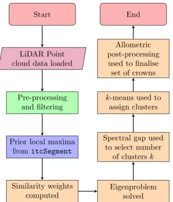
Fig. 1: MCGC tree crown segmentation algorithm. Here the colour of processes reflects the environment they have been coded in: LASTools are marked in green, R code is marked in blue and MATLAB code is coloured in orange.

B. The Multi-Class Graph Cut algorithm

The MCGC approach, summarised in Fig. 1, is explained in detail in this section. LAS data is first pre-processed and then the MCGC algorithm is applied to delineate tree crowns. Further post-processing based on knowledge of tree architectural geometry (i.e. allometric relationships) is then applied to ensure only sensibly shaped crowns are retained. A final double-layer extension is then explained.

1) Pre-processing and prior generation: The point cloud data are first cleaned using the LASTools package1_{. Points} marked as noise are removed and the lasheight method is used to generate a second point cloud with a model of the ground subtracted from the data points (based on points labeled as ground) to enable computation of above-ground height of points for prior generation.

The accuracy of the graph cut is improved by generating a lower bound on the number of expected tree crowns. This is estimated using the topography-corrected height point cloud and tree allometry information. Here we produced a list of expected tree-top positions computed by itcSegment — a local maximum finder that scales its search window size in relation to tree height used in the R packageitcSegment[27], [72]. Work presented here is completed using a rasterised canopy height model (CHM) gridded to 0.5 ×0.5 m pixels. A 50th percentile relationship between height and crown diameter was

1_{https://rapidlasso.com/lastools/}

used to set the size of the local search window based on the height of the CHM at that location. In this study the relevant relationship in (4) was always used in computing the prior. The number of local maxima exceeding a threshold of 5 m then sets a lower bound for the total number of trees to be found by MCGC. This height threshold was set to avoid inclusion ground returns and to avoid over-counting in areas of open canopy, where the search window becomes very small. As itcSegment only works on the top of canopy, it is expected to miss many lower canopy trees and so this number should be an underestimate. The MCGC approach, as outlined in Section II, requires a minimum and maximum number of tree (clusters) per plot to work with. The minimum matching the number of prior ‘trees’ and a maximum of twice this value was set. This choice was made to avoid forcing over splitting of crowns in the top, dominant layer of the canopy. We justify the suitability of this choice in the discussion in Section V-A1.

2) Graph cut: In what follows, we explain in detail the steps involved in our application of the MCGC graph cut algorithm introduced in Section II. The first step of the graph cut algorithm (implemented in MATLAB) converts 3D co-ordinates into a graph representation for all points above a minimum height of 2 m, to avoid ground returns being included. Here the raw height above sea level values are used to preserve the true structure of the vegetation. Working with topographically corrected data causes crown structures to be warped when the terrain is not flat as points are measured from the ground directly below them and not from the base of their respective tree stem [47]. In this work the 3D information in the LiDAR point cloud was used to construct weights to represent the similarity between points. The performance of graph cut approaches is contingent on the choice of weights,

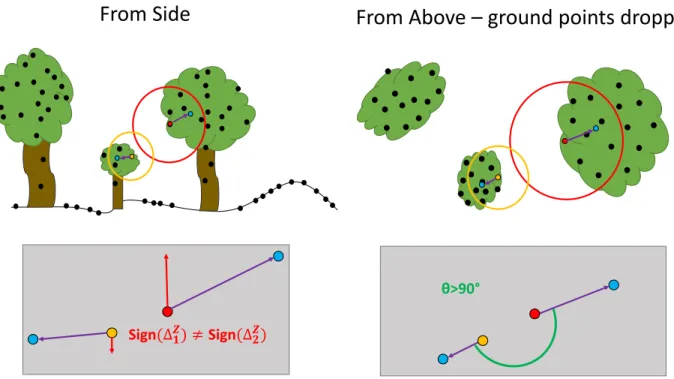
wij, and these must reflect the structure of segmentation targets to produce good results. Here we introduce a novel approach to assessing the similarity of points in a 3D point cloud for tree detection which avoids the need for prior determination of tree tops or stem locations and only uses the information within the structure of the point cloud. Our process captures knowledge of the basic geometry of the data and of the local density of points and how this relates to tree crowns. The key idea in using the local density of points is that for points near the external boundary of a crown, the local density of points constituting the crown should be higher than that of points outside the crown. This follows from a similar reasoning as used in [44] that trees should form local modes of point density in the data, but we extend this idea to focus on detecting the boundary of a crown. Computing a centre of mass (centroid) for the points in a neighbourhood of a boundary point should result in a point which lies roughly between the centre of the crown and the boundary point on which the neighbourhood is centred. Two nearby points on the boundary of the same crown should have their local centroids in a similar direction relative to the respective boundary points. In contrast, two boundary points on different crowns will have their local centroids located towards the middle of their respective crowns and so relative to the two boundary points, these will be orientated in different directions. Comparing the relative orientation of local centroids with respect to points

being compared should help distinguish crown boundaries. A simplified example of this principle is illustrated in Fig. 2 and a practical implementation on artificial data is shown in Fig. 3. As demonstrated in Fig. 3d, points on the opposite sides of a crown will also be penalised by this approach. For a single point, high similarities will only occur for links to points on the same side of the same crown and low similarities will result for points in neighbouring crowns and those on the opposite side of the same crown. Moving slightly around the crown, to neighbours of this point in the same crown, we see that points in other crowns still score low similarity, but the high similarity region of the desired crown, and thus the low similarity ’shadow’, changes, centring on the new point. Continuing this across the whole crown results in a well-connected set of points from the crown with strong links between mutual neighbours whereas neighbouring but distinct crowns have lower similarity scores to this entire set as no strong link exists to the crown of interest.

To encode the information from the local density of points into the similarity weights, the local centroid for each point was computed. The neighbourhood used was a sphere centred on the point in question with a radius based upon the above-ground height of the point in question. The radius of the sphere was based on the 95th percentile relationship in (4). To avoid the sphere extending beyond the stem location for boundary points in most trees the radius of the sphere was set to be half of the reference radius computed from the allometric relationship. This would capture most of the points in the relevant half of crown without extending too far and being skewed by other trees locally. The centroid of all points in this neighbourhood and the relative vector from the original point to its centroid, denoted by∆i for pointi, was then computed. In comparing points, the orientations of these relative vectors were compared. Points which belong to boundaries of different crowns would be expected to have vectors with very different orientations. Each of these vectors was broken down into horizontal and vertical components, denoted ∆H

i and ∆Zi respectively. Where the orientations suggested membership of different crowns, the similarity value (wij) was reduced. The process of computation of wij is outlined as follows (with wii = 0, ∀i). Note that it would be straightforward to introduce further similarity comparisons when constructing weights, such as comparing intensity values from imagery, similar to our work in [49], [58], but we have not done so here.

First, a basic similarity based on the distance between each pair of points is computed as

wbase ij = exp −||(x, y)i−(x, y)j||22 σ2 XY +−(zi−zj) 2 σ2 Z . (6) Here, wbase

ij in equation is separated into a horizontal (first exponential term in (6)) and a vertical component (second exponential in (6)). Each component can have its importance controlled by separate parameters as the vertical and horizontal structure and extent of crowns can vary for different forest types. The horizontal and vertical parameters are set before applying MCGC and are the same for all points (σxy andσZ

respectively). Here(x, y, z)i are the raw coordinates of point

i. An example of this is illustrated in Fig. 3b.

Next, the horizontal angle between the two centroid vectors ∆H

i and ∆Hj is computed as θH(i, j). When this is more

than a right-angle, the basic similaritywbase

ij is reduced. This reduction is based on the horizontal distance between the points, dH, so that closer points get a larger reduction in

similarity. This effect is normalised by a scale parameter,KH,

which is automatically set to the allometric radius for the tallest point in the data, using the 95th percentile allometry relationship in (4). Similarly, the larger the relative difference in the horizontal components of the centroid vectors, the larger the reduction in the similarity. The parameterWHcontrols the

overall importance of this modification relative to all other steps in the computation. An example of this reduction is shown in Fig. 3d. With this, the basic wbase

ij is updated to wpostHij as wpostHij = ( wH ij, if θH(i, j)>π₂, wbase ij , otherwise. wH ij =w base ij ×exp −WH KH dH ||∆H i −∆ H j||2 . (7)

Finally, the vertical components of the centroid vectors are compared (∆Z

i and ∆Zj). When these point in the same direction, no adjustment is made to the score. Where the directions differ, only pairs where these diverge have their weight reduced. Divergence occurs when the taller of the points has a positive ∆Z and the lower point a negative one. This would be expected for points in different crowns of varying height, whereas points at the top and bottom of the same crown would expect to have vertical components that point towards a central point in the crown. As with the horizontal comparison, this reduction is larger for points which have a smaller vertical distance,dZ, between them. The

normalisation for this, KZ, is set to half of the aboveground

height of the tallest point of the data. The reduction is also larger when the relative difference in the vertical centroid vectors is larger. An example of this reduction is shown in Fig. 3e. With this, the final similarity weights,wij, as shown in Fig. 3c, are computed as

wij= ( wZ ij, if ∆ Z i and∆ Z j diverge, wpostH_ij , otherwise. wZ_ij= wijpostH×exp −WZ KZ dZ |∆Z i −∆ Z j| . (8)

Calculating pairwise weights for every set of two points would be computationally cumbersome, producing a matrix of weights that is far too large to store in a typical computer’s memory (≤ 16 GB RAM). As an indication, a point cloud of 40,000 points would require 12.8 GB of RAM to be held in memory, ignoring overheads and the need for spare memory to perform the necessary computations, which at the point density of the Sepilok dataset would cover roughly 0.25 ha. To resolve this issue, the Nystr¨om extension is used [73]. Here the complete matrix and relevant eigenvectors are

Sign

(∆

_𝟏𝒁

) ≠

Sign(∆

_𝟐𝒁

)

θ

>90°

From Above

–

ground points dropped

From Side

Fig. 2: Simplified illustration of the principle of the local density centroid calculations. Points being compared are red and orange, with associated neighbourhoods shown. Blue points are centroids for each neighbourhood, with centroid vectors in purple. Comparisons of these vectors are then shown in the grey boxes. In this example both comparisons would result in a reduction in the similarity weight between the highlighted points. Here the illustration shows how the horizontal and vertical directional differences in the centroid vectors distinguish the points highlighted as belonging to distinct crowns.

computed for a subset of the points, typically less than 10% of the data. The eigenvectors are then extended to the full dataset through quadrature based on the weights in a manner that produces a robust approximation of wij [73], [74]. This allows computation of all pairwise weights for the subset and avoids a need for a sparse representation of the pairwise linkages. Computationally, we found computing eigenvectors takes much more time than computing a complete graph (where all points are linked to all other points). Thus the Nystr¨om extension approach is more efficient than trying to compute complete eigenvectors on a sparse version on the graph.

3) Using crown allometry to refine the segmentation: An extension of the basic graph cut algorithm makes use of knowledge of crown radius scaling with tree height to remove improbable trees, by post-processing of clusters identified by the initial graph cut. For a candidate tree in the segmented dataset, a ‘maximum’ predicted crown radius was taken from look-up table based on its height. The numbers in the look-up table were based on the 95th percentile relationship from the global database in [56] as given in (4). Any crowns which exceeded the range of this dataset were set to match the maximum allometric radius for the dataset. The horizontal top of a tree was approximated as the mean position of all points with aboveground height of 98% or greater of the top point. First candidate crowns that overlapped too much with larger

neighbours, both in horizontal extent and vertical overlap were merged. We define excessive horizontal overlap as when either the top or more than 60% of the points of a tree are within the allometric radius of a taller tree. The threshold of 60% was chosen to be a balance between ensuring a majority of points in a candidate crown need to be within the region but also avoiding ignoring all but significantly overlapping candidate crowns. This threshold was set as part of the algorithm and not treated as a parameter. Excessive vertical overlap is when the top quartile of heights in a crown overlap the bottom quartile in a taller crown. This approach was chosen as a non-parametric approach based solely on quartiles. This was also set before analysis and not treated as a parameter. Crowns are only merged if both horizontal and vertical overlap are excessive. Then crowns where more than 5% of points lie beyond the computed maximum radius from the tree top are further trimmed. This cut-off is set to match the radius being used, here being a 95-th percentile relationship. This was also set before analysis, again not being treated as a parameter. Trimming uses hierarchical clustering based on the Euclidean distance between points, using raw heights. Two clusters are produced and the one which includes the tree top is kept, with points in the other cluster added to the rejected points list. Finally crowns which contain too few points were rejected, with a threshold of a minimum of 100 points per crown. This was set to filter crowns which were missing many points and to

(a)

(b)

(c)

(d)

(e)

(f)

Input Data

Base Similarity Weights

Density-adjusted Weights

Horizontal Gradient Term

Vertical Gradient Term

Double Layer MCGC Output

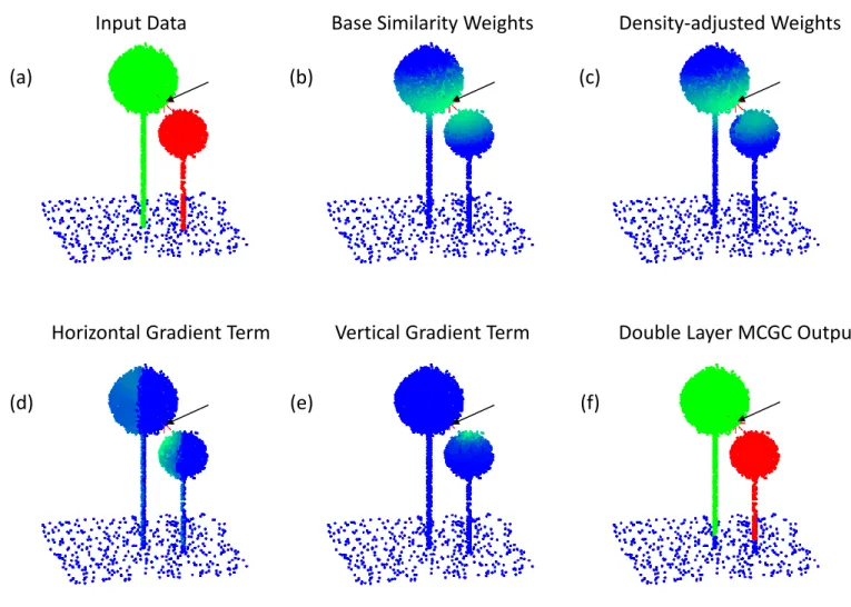
Fig. 3: MCGC applied to artificial trees to explain the role of centroid vector computations in segmentation. The relative effect of applying the centroid adjustments when comparing to the marked point are shown in panels (d) and (e), and this is reflected in the weights as shown in panels (b) and (c), where the closest points on the smaller crown have weaker links than the base weights, with minimal difference made to points in the taller crown. Panel (a) shows two simulated trees with allometry matching that of the 50th percentile for crowns in Indo-malaya where the green tree is 30 m tall and red tree is 20 m tall with blue points being the ground. Panel (b) shows the qualitative distribution ofwbase

ij for each point computed with reference to the crown boundary point highlighted by an arrow in all panels, centred at the red star; higher values are represented by green in the blue-green colour ramp. Panel (c) shows the distribution of wij once the centroid adjustments have been made. The colour ramp is the same and shows the reduction in similarity to the neighbouring crown whilst preserving linkages to the target crown. (d) shows the effect of the modification based on horizontal components of centroid vectors in (7). Dark blue represents minimal adjustment to the weight and lighter colours represent a greater reduction in weight. (e) shows the same effect as in (d) when looking at the adjustment based on the vertical component of the centroid vectors in (8). (f) shows the output of double-layer MCGC, with each crown highlighted in a different colour, with unclassified points in blue, recovering the true structure in (a) with the exception of the bottom 2 m of the stem, as this was the height threshold set.

avoid the trimming step from causing crowns to be too small. The goal here is to ensure only allometrically feasible crowns are kept, with all other points being marked as not contained within a crown. These points are rejected in this application of graph cut.

4) Detecting lower-canopy trees: The allometric refinement stage leads to there being points which are not assigned to any tree. These can be from trees which are close neighbours of successfully detected crowns where removal of this crown

makes delineation easier. Equally many of these points are in the understorey, where point densities are lower due to occlusion and differentiation of crowns is more challenging. A second pass of MCGC is then used to detect tree crowns from the unassigned points. These trees are then added to those accepted in the first application of MCGC to produce the final list of crowns. It is possible to alter the weight parameters to reflect differences in the canopy structure in these lower layers; however we applied the MCGC algorithm with the same set

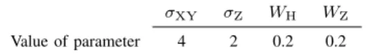
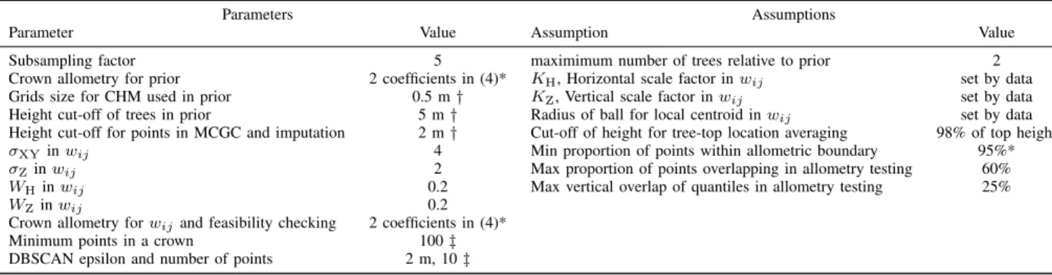
TABLE I: Values of Parameters Selected for MCGC by Trial and Error

σXY σZ WH WZ Value of parameter 4 2 0.2 0.2

of parameters in the second pass in this study. This simple extension is illustrated in Fig. 4.

5) Selecting parameters: The values ofσXY,σZ,WHand

WZ in (6) – (8) control the relative importance assigned to

each component in computing similarities between points. To set these, nine of the 36 1-ha plots were used, three from each soil type, comprising 25% of the data in this study. To decide the best choice of parameters from those trialled, the resulting segmentations were manually inspected, and the distribution of detected crown sizes was qualitatively compared to the distribution of field inventory stem sizes for the 9 plots. We chose not to automatically tune the parameters based on biomass estimates as this would be likely to falsely remove any bias, possibly by allowing unrealistic crown delineation. An automatic method to assess accuracy of tree shape could be used for a robust selection with a more detailed field inventory. First the values of σXY and

σz were simultaneously assessed, by trying MCGC with each parameter taking one of a number of values and trying all possible pairings. For this process, the modifications in (7) and (8) were not applied to any weightings. It was expected that the vertical distance would need a smaller parameter, penalising this more heavily, as tropical crowns are often wide and less vertically extended than the typical conic shape of coniferous forests [56]. Analogous parameters in previous work on the use of graph cut on coniferous forests found the horizontal parameter to be the smaller, following the same reasoning [49]. Similarly to the first two parameters,WH andWZ were

simultaneously trialled in an exhaustive manner, withσXYand

σZ set to their selected values. The final parameters used in

this study are listed in Table. I.

C. Improving computational efficiency

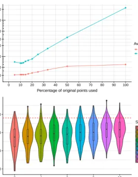
As shown in Section II, applying the graph cut algorithm amounts to solving an eigenvector problem. Such problems do not scale well with increasing matrix size. The Nystr¨om extension already reduces the effective matrix size used in the algorithm. However, as the number of points in the dataset increases, the total memory required still increases. To resolve this only with the Nystr¨om extension would require taking a very small subset of points for applying the approximation. Instead, when working with datasets of 1 ha or more a simple method for reducing the workload was developed, by downsampling the data and then imputing the full data results. This can be justified as the dense point cloud is locally correlated – points close in horizontal extent will have similar height values and a subsampled point cloud retains the 3D structure of the dense data. This way the MCGC algorithm is applied in full to a subsampled point cloud and the Nystr¨om extension can be applied at the same proportion of points used

in MCGC for datasets over large areas, or from very dense ALS data. The full pre-processed point cloud is downsampled, by random (without replacement) sampling of the data. The Multi-Class Graph Cut is then applied to this subset. Once the crowns are identified, the full dataset is then imputed by a m-nearest neighbour approach. The value of m is set to match the effective downsampling, so if 1/5 of the data is used thenm= 5is used for imputation. For a given crown, points could only be added to it in imputation if they lay within the maximum allometric radius of this crown, as computed from the 95th percentile relationship in (4) for the height of this crown. To ensure imputation did not create artefacts, where rejected crowns were now grouped with their nearest valid crown, the DBSCAN algorithm was applied to each final tree [75]. This finds groups of points for which there are at least 10 other points within 2 m. A neighbourhood is then constructed of all neighbouring points which satisfy this property, as well as all points within 2 m of this group. This ensures imputed crowns are formed of a single locally-connected group of points and any points not connected to this were marked as unassigned. In this work we used a subsampling pool of 20% of the data. In the double-layer extension, subsampling and imputation was applied to each application of MCGC, applying it twice in the pipeline. We explored varying or removing subsampling in the second pass of MCGC, as returns in the lower canopy are more sparse owing to occlusion. We found results are generally stable for using 20% of the data or more, with detail set out in Appendix A. In running the full double-layer MCGC algorithm to all 36 one ha plots in this study, the total time taken averaged 66,250 s. This is equivalent to the algorithm taking 30 m 40 s per plot. This timing was completed on a workstation running Windows 7 using MATLAB 2017a. The workstation was equipped with an Intel Xeon E3-1240 V2 CPU, comprising 8 cores running at 3.4 GHz with 16 GB RAM. MATLAB allocates memory smartly to enable calculations to proceed where theoretically they may be RAM-limited. Accordingly, running the MCGC algorithm on a machine with more RAM, or where subsampling is optimised to adapt to the RAM restrictions of a machine has the potential to accelerate the algorithm, but we do not explore that option in this work.

D. Assessment of segmentation accuracy

MCGC was applied to the 36 1 ha plots within the Sepilok dataset. The two versions outlined in Section III-B of the al-gorithm were tested: (1)single-layer MCGCapplied a single graph cut to the data followed by the allometric filtering (as per Fig. 1); (2)double-layer MCGC extended the results of this by applying a second pass of the algorithm to unassigned points (as per Fig. 4).

To compare the distribution of trees found by the automatic detection methods, the diameter at breast height (DBH) of these were estimated. This metric was previously recorded in the Sepilok data set for all stems, whereas their heights were scarcely recorded. To convert from remotely sensed height to DBH, log-log regression was applied to the 91 trees manually

Graph Cut

Graph Cut on

remaining

points

Allometric

Testing (leaving

some points)

Combine all

trees found in 2

passes

Allometric

Testing

(rejecting some

points)

Fig. 4: Pipeline for double-layer approach to MCGC

delineated by Coomes et al. [27]. This results in the following relationship for H(m) and DBH(cm):

DBH = 0.252×H1.465 ₍₉₎

DBH for each tree crown detected by the MCGC algorithms was estimated from their above-ground height using this relationship. The results were then compared by grouping stems into a number of diameter classes and comparing the number of stems in the field inventory and the number of stems predicted by MCGC.

E. Predicting biomass

Field surveys are commonly used as a basis for estimating carbon stored in above-ground biomass. Accordingly we com-puted biomass estimates for the trees in each plot to measure the total estimated above-ground carbon density for each 1 ha plot (ACD, Mg ha−1

). For each plot we compared the total ACD from the field survey to that from each of the MCGC based methods. Here AGB was computed for each tree, and these values were then summed for each plot. Finally a conversion factor of 0.47 was applied to convert from AGB to ACD [76].

For the field survey, the biomass from each tree in the forest inventory was computed according to Chave et al.’s pantropical equation [77]:

AGBfield= 0.0673×(WD×D2×H)0.976, (10)

whereWDis the wood density as taken from the global wood density database [78], [79], D is the stem diameter (cm) and His the estimated height (m) based on (5). Wood density was mapped to the best taxonomic unit available for each species. If there was no data for a species, then the average for its genus was used, and similarly where there was no data for this the family average was used. If there was no data at family level, an average of all species present in the Sepilok plots was used. The AGB per plot was then computed by summing the contribution from each tree before being converted to ACD.

The ACD contribution of each automatically segmented tree was computed using the following relationship, originally derived by Coomes et al. in [27] from 91 crowns manually delineated and verified in the LiDAR data:

ACDauto= 0.268×(H×CD)1.45, (11)

where H is the aboveground height of the segmented tree (m) and CD is the crown diameter (m) computed from the crown area (CA) as CD = 2×p

CA/π. For the MCGC output, the crown area was taken to be the area of the convex

polygon enclosing each tree. Comparisons between the ACD estimates from the field inventory and remote sensing methods were compared for each one ha plot. Overall results are then reported via the bias and Root Mean Square Error (RMSE) of the predictions. These were computed as a percentage of the predictions of ACD for the field inventory data. Here a negative bias indicates the remote sensing estimate is an underestimate.

Previous work on automatically detected individual-based AGB estimation notes that often this systematically under-estimates biomass as trees in the lowest layers of the canopy are rarely detected [20], [27]. In [27], using the same data as in this study, trees with a DBH below 30cm account for 23% of the total biomass across all plots. It can therefore be infor-mative to apply a simple linear correction factor to account for this. In [27] this was applied both to all plots simultaneously and with a different correction factor for each forest type. Similarly, in [45] the AGB at plot level is computed by applying a multiplicative constant to the sum of estimated AGB for each crown. As we found our overall estimate of ACD from double-layer MCGC was already low-bias overall we chose to only compute a forest-type specific correction factor. This can be justified as the MCGC algorithms here used only a regional allometry which was based on data for the whole Indo-Malaya region in (4) with no local allometric input for the MCGC algorithm. A forest-type specific correction was computed by fitting a linear regression model to the ACD estimates from MCGC and the field inventory for the 12 plots of each forest type, constrained to pass through the origin.

F. Comparison to existing methods

MCGC was directly compared to two existing algorithms as a benchmark of performance. The itcSegment algorithm as implemented in [27] was used as a reference ITC algorithm. This is applied to the rasterised CHM, computed at a 0.5 m resolution. First a moving window local-maxima finder detects tree tops, where the size of the window scales with above ground height in the same manner as our prior generation step does. Finally trees are delineated by a region-growing algorithm taking the local maxima as seed points. Data from this algorithm were processed in the same way as those from MCGC as outlined in Sections III-D and III-E. Estimation of AGB was further compared to an area-based model [80]. This predicts biomass at one ha scale based on metrics of the CHM. The approach uses the general biomass equation from [80] for which ACD is computed for a one ha plot asACDGeneral =

3.836×TCH0.281×BA0.972×WD1.376, where TCH is mean top canopy height (m), BA is basal area (m2_ha−1

diameter-weighted mean wood density (g cm−3_{). To estimate}

BA and WD from the ALS data the approach used in [27] was applied, where both were estimated as power laws of TCH based on the 36 one ha plots to give an overall model for ACD asACDGeneral= 7.37×TCH0.870. Following the suggestions

in [80] and replicating the approach in [27] a locally-fitted area-based model was also used. This takes the same form as the general model but with the powers and multiplicative factor directly fitted to the Sepilok plots but log-log regression. Further, following the work in [27], BA was predicted not from TCH, but instead from Gap Fraction at a height of 19 m (GF19). This counts the number of pixels in the CHM raster

for which the TCH is below 19m as a percentage of all pixels in the raster. Brought together these produce a locally-fitted model for ACD asACDLocal= 25.93×TCH0.437×GF−190.209.

IV. EXPERIMENTALRESULTS

A. Tree detection

Single-layer MCGC detects many of the largest trees, but misses intermediate and lower layers of the canopy. The additional detection of trees in double-layer MCGC is evident in the example results for one plot of each forest type shown for each method in Fig. 5. Fig. 6 shows the comparison between the field survey measurements and MCGC-estimated DBH values broken down by bands of diameter and detection rates by diameter class are summarised and compared with the results from using itcSegment in [27] in Table. II. Single-layer MCGC under-estimated the number of trees across all diameter classes (Fig. 6a). This results from a strict set of allometric testing criteria, where clusters that don’t pass are rejected. Thus under-estimation of even the tallest trees can be expected. In this case, many of the tallest trees are accounted for (69.8% of trees with DBH>110 cm and 62.8% of those with 90 cm<DBH<110 cm). However, when compared to the same counts for itcSegment, which works only on the top canopy surface, (103.2% and 82.2% respectively) it is clear single-layer MCGC does not account for all trees in the top layer as these are being detected by itcSegment. For all trees with DBH of 90 cm or smaller a single application of MCGC detects fewer than half the number of stems recorded in field inventory, and itcSegment outperforms single-layer MCGC. These trees account for the vast majority of total stems though many will be in the intermediate layers of the canopy. This motivates and justifies applying the algorithm a second time to detect these intermediate layer trees with many of the largest trees already confidently detected.

Once a second pass of MCGC was applied in the double-layer MCGC pipeline (Fig. 6b) the number of trees found increased across all diameter classes. This leads to some overestimation in the tallest classes (128.6% for DBH>110cm and 137.2% for 90 cm<DBH<110 cm) but leads to much better estimates of trees in the intermediate size ranges (87.4% for 70 cm<DBH<90 cm and 56.6% for 50 cm<DBH<70 cm). These detection rates are comparable to, or improvements on, itcSegment for the same size stems (51.8% and 61.9% respectively). Double-layer MCGC still misses most of the trees in the lowest canopy layers (29.9% for 30 cm<DBH<50

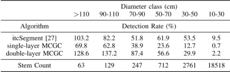
TABLE II: Summary of Detection Rates by Diameter Class for MCGC and itcSegment with stem count by diameter size class for the field inventory data. A dectection rate of 100% means a count exactly matching that of the field inventory and values above 100% show oversegmentation and values under 100% undersegmentation

Diameter class (cm)

>110 90-110 70-90 50-70 30-50 10-30 Algorithm Detection Rate (%)

itcSegment [27] 103.2 82.2 51.8 61.9 53.5 9.5 single-layer MCGC 69.8 62.8 38.9 23.6 12.7 0.7 double-layer MCGC 128.6 137.2 87.4 56.6 29.9 2.2 Stem Count 63 129 247 712 2761 18518

TABLE III: Bias and RMSE for AGB estimates from MCGC, itcSegment and Area-based Modelling for both original model output and once a forest type specific correction factor has been applied to MCGC and ITC and the area-based model has been locally calibrated

Original Specifically Calibrated Algorithm Bias (%) RMSE (%) Bias (%) RMSE (%)

itcSegment [27] -20 26 -1 18

Area-based Modelling [27] -19 20 0 13

single-layer MCGC -48 36 3 21

double-layer MCGC -0 33 -2 18

cm and 2.2% for 10 cm<DBH<30 cm). In these classes of stem size itcSegment reports a higher number of stems though itself still misses a large proportion of stems (53.5% and 9.5% respectively). For all diameter classes where DBH<90 cm, adding a second pass of MCGC more than doubles the counts of stems found by single-layer MCGC which means more trees in these diameter classes are found in the second application of MCGC than are found in single-layer MCGC alone.

B. Biomass estimation

Single-layer MCGC underestimated biomass of all three forest types (bias: -48%, Fig. 7a and Table. III) and including a second pass of MCGC removed the overall bias in estimating plot ACD Fig. 8a and Table. III). This is consistent with the comparison of stem counts in Fig. 6a which showed that the single-layer MCGC approach underestimated stem sizes across all classes. Including a second pass of the MCGC algorithm removed the overall bias in the predictions (Fig. 8a). However, this resulted from a tendency to overestimate biomass in the Alluvial forest type matched with small underestimation in both Kerangas and Sandstone forest types (Table. IV). Underestimation can be accounted for by missing trees in the lower canopy. Alluvial forest contains almost all of the tallest trees in Sepilok and so the tendency of double-layer MCGC to over-detect these explains the overestimation of ACD in these plots. Both approaches had a relatively large RMSE (36% and 33%) but this is not unexpected in an individual tree approach to estimation of biomass as big trees contain a large proportion of the total biomass. Small errors in prediction of the largest trees can therefore have a large effect on overall predictions

(a) (b) (c) (d) (e) (f) (g) (h) (i) Alluvial Sandstone Kerangas

Raw Data MCGC Single Layer MCGC Double Layer

Fig. 5: Example results of applying MCGC single-layer and MCGC double-layer to a 1 ha plot of each forest type. Each row represents a plot of one of the three soil types: Alluvial (a–c), Kerangas (d–f) and Sandstone (g–i). Across each row are the raw data (coloured by height), the output from single-layer MCGC (coloured by crown) and the output from double-layer MCGC (coloured by crown). Points which are unassigned are not included in the MCGC output images and the increased detection of trees can be seen by comparison between the second and third columns: pairs b & c, e & f and h & i.

TABLE IV: Bias and RMSE for AGB estimates from MCGC, itcSegment and Area-based Modelling based on original model output broken down by forest type

Alluvial Forest Kerangas Forest Sandstone Forest Algorithm Bias (%) RMSE (%) Bias (%) RMSE (%) Bias (%) RMSE (%)

itcSegment [27] -14 20 -19 9 -29 18

Area-based Modelling [27] -3 15 -21 8 -30 13

single-layer MCGC -26 23 -58 17 -60 22

double-layer MCGC 39 22 -18 14 -21 16

of AGB and ACD. By comparison, in the original study by Coomes et al. in [27], the general area-based approach for estimating ACD, as per [80], produced predictions with a bias of -19% and RMSE of 20% (Table. III). The ITC approach in this study produced ACD predictions with a bias of -20% and RMSE of 26% (Table. III). When looking at the contributions of individual forest types, the methods in the original study produce closer estimates for Alluvial forest types, as a result of the overestimation by double-layer MCGC (Table. IV). In contrast, for both Kerangas and Sandstone forest, double-layer

MCGC produces closer estimates to the field inventory than any of the other methods considered here.

Appplying a correction factor for each forest type reduced overall bias and error. For single-layer MCGC the correction factors were larger than 1 as expected given the algorithm underestimated ACD (Alluvial 1.32, Sandstone 2.40, Kerangas 2.30, Table. V). Double-layer MCGC had correction factors that showed an underestimation of ACD in Kerangas and Sandstone forest matched with a similar overestimation in alluvial forests (Alluvial 0.70, Sandstone 1.24, Kerangas 1.21,

10−30 30−50 50−70 70−90 90−110 >110

Diameter class (cm)

log (Number of trees)

0 2 4 6 8 10 0.7% 12.7% 23.6% 38.9% 62.8% 69.8% single−layer MCGC (a) 10−30 30−50 50−70 70−90 90−110 >110 Diameter class (cm)

log (Number of trees)

0 2 4 6 8 10 2.2% 29.9% 56.6% 87.4% 137.2% 128.6% double−layer MCGC (b)

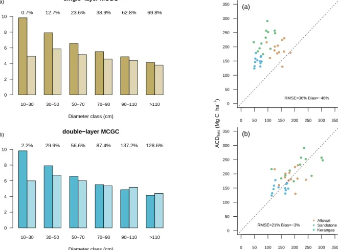
Fig. 6: Comparison of log-transformed numbers of trees by stem diameter for field inventory, left and dark, and each MCGC implementation, right and light. Percentages are given for MCGC as fraction of field inventory. MCGC methods are: (a) single-layer MCGC, (b) double-layer MCGC. Applying the second round of MCGC increases detection rates across all stem size groups and more than doubles the rate of detection in stems of a size of 90 cm or less.

TABLE V: Linear correction factor computed for each forest type when AGB estimates are compared to field inventory

Correction Factor

Algorithm Alluvial Forest Kerangas Forest Sandstone Forest

itcSegment [27] 1.07 1.32 1.30

single-layer MCGC 1.31 2.30 2.40

double-layer MCGC 0.70 1.21 1.24

Table. V). Applying this correction removed the bias for single-layer MCGC (3% vs 48%), but only reduced the bias within each forest type for double-layer MCGC as this already had low overall bias (Table. III). In both cases this reduced the RMSE as any bias for each forest type was reduced independently (21% vs 36% and 18% vs 33% for single-layer and double-layer MCGC). The effect of these corrections are similar for itcSegment, removing bias and reducing RMSE, as reported in [27] and shown in Table. III. When choosing to

● ● ● ● ● ● ● ● ● ● ● ● ● ● ● ● ● ● ● ● ● ● ● ● ● ● ● ● ● ● ● ● ● ● ● ● 0 50 100 150 200 250 300 350 0 50 100 150 200 250 300 350 (a) RMSE=36% Bias=−48% ● ● ● ●● ● ● ● ● ● ● ● ● ● ● ● ● ● ● ● ● ● ● ● ● ● _● ● ● ● ● ● ● ● ●● 0 50 100 150 200 250 300 350 0 50 100 150 200 250 300 350 ● ● ● Alluvial Sandstone Kerangas (b) RMSE=21% Bias=−3% ACDLiDAR (Mg C ha −1 ) A C Dfi e ld (Mg C h a − 1)

Fig. 7: Comparison of field-estimated above-ground carbon density (ACDfield) with estimates based on single-layer Multi-Class Graph Cut (ACDLiDAR) for each of the 36 one-ha subplots. Panel (a) shows the original estimates with a 1:1 line (dashed). (b) shows the effect of applying a linear forest type specific correction factor to ACDLiDAR.

use a locally-calibrated model for the area-based approach the same effects are seen again. Here the model has all parameters for AGB as a function of remotely sensed variables directly fitted to the field inventory data, and the Gap Fraction height is chosen that best predicts Basal Area when compared to field inventory data [27]. Accordingly there is not an obvious analogue of the single correction factor that can be compared as is possible for itcSegment and MCGC (Table. V).

V. DISCUSSION

A. Assessment of MCGC Performance

1) Forest inventory: When comparing the distribution of stem sizes found by single-layer MCGC to the reference field inventory it is clear that across all stem sizes the algorithm did not find all individual trees (Fig. 6a). The initial graph cut segmentation is constrained to find at least as many crowns as a simple maxima finding algorithm. As shown in Table. II, the itcSegment algorithm, which starts with the same local maxima approach finds more than 50% of the count of stems for trees with DBH>30 cm. These totals represent the number

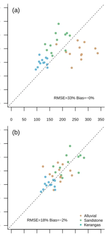
● ● ● ● ● ● ● ● ● ● ● ● ● ● ● ● ● ● ● ● ● ● ● ● ● ● ●● ● ● ● ● ● ● ● ● 0 50 100 150 200 250 300 350 0 50 100 150 200 250 300 350 (a) RMSE=33% Bias=−0% ● ● ● ● ● ● ● ● ● ● ● ● ● ● ● ● ● ● ● ● ● ● ● ● ● ● ●● ● ● ● ● ● ● ● ● 0 50 100 150 200 250 300 350 0 50 100 150 200 250 300 350 ● ● ● Alluvial Sandstone Kerangas (b) RMSE=18% Bias=−2% ACDLiDAR (Mg C ha −1 ) A C Dfi e ld (Mg C h a − 1)

Fig. 8: Comparison of ACD estimates by plot for double-layer MCGC for each of the 36 one-ha subplots. ACDfieldand ACDLiDAR are the ACD estimates from the field survey and from MCGC applied to LiDAR data respectively. (a) shows the original estimates with a 1:1 line (dashed). (b) shows the effect of applying a linear forest type specific correction factor to ACDLiDAR.

of local maxima initially found as itcSegment is constrained to delineate one tree for each local maximum. From this single-layer MCGC then found fewer stems than itcSegment. The graph cut step is constrained to find at least as many trees as the initial prior number of trees. Therefore the underestimation likely stems from the allometric filtering step. This step applies multiple criteria to each crown, based on knowledge of a regional allometry, rejecting those crowns that do not meet the criteria closely enough. This results in a reduction of the number of crowns, but those that remain are allometrically feasible. Notably, the algorithm finds a greater proportion of crowns relative to itcSegment in the largest classes (DBH>70 cm) than the smaller classes, suggesting that the rejection of crowns may be more common for medium and small trees.

Double-layer MCGC detects more tree crowns in all diam-eter classes (Fig. 6b and Table. II). These additional crowns are detected in the second application of the MCGC algorithm. The algorithm over-detects the number of trees in the largest diameter classes (DBH>90 cm), though there are fewer trees

of these sizes, meaning the over count is not a large number of trees compared to the total count of all stems. As a trade-off, double-layer MCGC is able to detect more than double the number of trees in all small and medium classes (DBH<90 cm) when compared to the single-layer approach. This reduces the under counting in these diameter classes. This results from the ‘stripping-off’ of the dominant trees to allow the algorithm to better segment the under layers of the canopy. However the algorithm struggles with finding the smallest trees as is a drawback of working with ALS data [27]. The number of returns for these trees is very small and this underlines the importance of alternative approaches, such as using TLS data, for mapping the lowest layers of the canopy. Overall double-layer MCGC is able to detect most crowns for intermediate and large sized trees.

Results from the itcSegment approach in [27] justify the choice of limits for the choice of total tree stems. These limits are set to a minimum of the number of local maxima itcSegment would find and a maximum of twice this. From Table. II it is clear that itcSegment underestimates the number of crowns in all but the largest stem class. Therefore the total number calculated in this way will be an underestimate, though estimates well for trees of DBH>90 cm. Equally, for all stems where DBH>30 cm, itcSegment finds at least 50% of the total number of stems for each diameter class. Therefore doubling the number of local maxima found by the first step of this algorithm should over estimate the number of stems in all diameter classes where DBH>30 cm. This would then make a sensible upper limit for the number of crowns to seek for crowns of this size. For trees where DBH<30 cm all such approaches result in under-counting of stems. These trees are mostly found in the lower layers of the canopy and, as discussed below, this is a persistent problem with ALS data. Thus increasing the upper limit of crowns sought is more likely to lead to worsened over-segmentation of the largest crowns than to aid in finding these elusive smaller trees.

The difficulty of finding trees in the lowest layers of the forest canopy is a persistent problem in analysing ALS data in multi-layered canopies [26], [27], [34]. Here occlusion causes a diminishing number of returns for lower canopy, making it hard to identify the smallest trees in the subcanopy, even when inspecting the data visually [26], [34]. This highlights the importance of taking a combined approach to data collection, pairing ALS data acquisition with other methods such as TLS or field inventory. These methods themselves suffer from limitation in scope of the area they can cover when compared to ALS in the same time frame [7]–[9]. When working on locations of many hectares and larger, being able to automatically estimate the number of stems in the dominant canopy layers is a very useful tool and double-layer MCGC is able to provide this across several distinct forest types in the tropics.

2) Biomass estimation: Single-layer MCGC underesti-mated 1 ha plot-level carbon density (Fig. 7a). This is consis-tent with the under-detection of crowns discussed in Section V-A1. The bias of -48% shows that the estimates of biomass are about half of the values calculated based on field inventory, which is not unexpected. The algorithm finds more than half