A COMPARATIVE STUDY OF METHODS FOR DEFECT
DETECTION IN TEXTILE FABRICS
1 2 2
P. NSENGIYUMVA, H. VERMAAK & N. LUWES
1
UNIVERSITY OF RWANDA, COLLEGE OF SCIENCE & TECHNOLOGY
2
CENTRAL UNIVERSITY OF TECHNOLOGY, FREE STATE, SOUTH AFRICA
Abstract
Fabric defect detection methods have been broadly classified into three categories; statistical methods, spectral methods and model-based methods. The performance of each method relies on the discriminative ability of texture features it uses. Each of the three categories has its own advantages and disadvantages and some researchers have recommended their combination for improved performance.
In this paper, we compare the performance of three fabric defect detection methods, one from each of the three categories. The three methods are based on the grey-level co-occurrence matrices (GLCM), the undecimated discrete wavelet transform (UDWT) and the Gaussian Markov Random field models (GMRF) respectively from the statistical, spectral and model-based categories. The tests were done using the textile images from the TILDA dataset. To ensure classifier independence on the outcome of the comparison, the Euclidean distance and feedforward neural network classifiers were used for defect detection using the features obtained from each of the three methods. The results show that GLCM features allowed better defect detection than wavelet features and that wavelet features allowed better detection than GMRF features.
Keywords: Grey-level co-occurrence matrix, wavelet transform, Markov random field, Euclidean distance classifier, neural networks
1. INTRODUCTION
Quality inspection of textile products is an important issue for fabric manufacturers. Manual fabric quality inspection by human inspectors has many drawbacks - including fatigue, boredom, inconsistency and low detection rate. Many attempts to automate this task have been made and various defect detection methods have been proposed in the literature. Kumar
(2008) and Ngan et al. ( provided recent reviews of research in this field.
Most of the methods view the problem of fabric defect detection as a texture classification problem and rely on the discriminative ability of texture features for their performance.
Weszka et al. (1976) and Conners et al. (1980) undertook comparative studies of the performance of four texture algorithms as well as their respective features. While the former was performed experimentally on terrain sample images, the latter was theoretical. The four methods were Grey-Level Co-occurrence Matrix (GLCM), Level Run-Length Method (GLRLM), Grey-Level Difference Method (GLDM) and Power Spectrum method (PSM). Both studies concluded that GLCM was more powerful than the other three considered methods while GLDM was more powerful than PSM. Bodnarova et al. (2000) compared the performance of four methods of detection of weaving defects, namely grey-level co-occurrence, normalized cross-correlation, texture blob detection and spectral methods, in terms of detection accuracy and computational efficiency. They claim that cross-correlation was the most promising method for textile fabrics.
The purpose of this paper is to compare the performance of three fabric defect detection methods. The three methods are based on the grey-level co-occurrence matrices (GLCM), the undecimated discrete wavelet transform (UDWT) and the Gaussian Markov Random field models (GMRF). The comparison provides a platform for their combination for increased performance. The remaining part of this paper is organized as follows. In Section 2, we describe the feature extraction methods used, namely GLCM, UDWT and GMRF. In Section 3, we briefly describe the Euclidean distance and the feedforward neural network classifiers that we used as defect detectors. Section 4 provides an overview of the dataset and the experiments while Section 5 presents the results as well as their interpretation. Our conclusions are reached in Section 6.
2. FEATURE EXTRACTION METHODS 2.1 The Grey-Level Co-occurrence Matrices
The grey-level co-occurrence matrix (GLCM) analysis was introduced by Haralick et al. (1973). It is a second order statistics method of texture analysis in the sense that it is based on the computation of statistics of pairs of neighbouring pixels in an image, separated by a given distance d in a given direction .
A co-occurrence matrix is a square matrix whose elements are the number of occurrence of pairs of grey levels separated by the distance d in the direction . For an image with G grey levels, the grey-level co-occurrence matrix P is a
GxG matrix and its element P (p,q) can be expressed by (1).d,
Ɵ
Ɵ
In general, four such matrices are used to describe different orientations in an image. More specifically, one co-occurrence matrix describes pixels that are
0
adjacent to one another horizontally, P . There are also co-occurrence
90 45
matrices for the vertical direction and both diagonal directions called P , P
135
and P respectively.
0
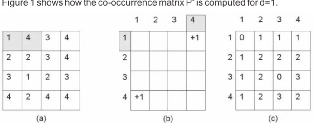
Figure 1 shows how the co-occurrence matrix P is computed for d=1.
0
Figure 1: Construction of the co-occurrence matrix P for d=1 (Miyamoto et al., 2005) The original image (a) begins by having each of its neighbouring pairs examined. (b) shows the incremental stage that occurs when the outlined neighbouring pixels in (a) are examined. Part (c) shows the final result of the horizontal co-occurrence matrix for d=1 (Miyamoto et al., 2005).
After compiling the co-occurrence matrix, some features are calculated from it. We will consider all fourteen features as proposed by Haralick et al. (1973).
2.2 The Gaussian Markov Random Field models
The model used is as described by Cohen et al. (1991). Let g (m,n) be the 0
intensity at pixel r = (m,n) and let g(m,n)= g (m,n)-µ where µ=E{g (m,n)}. The 0 0
GMRF is a noncausal 2-D autoregressive process described by the difference equation (2)
where p is the order of the process and Np is the maximum square of distance from r to v. n(r) is a Gaussian noise sequence with zero mean and autocorrelation function given by equation (4).
The GMRF is parameterised by a parameter set γ = (µ,σ, β) with β = (β10,β01,β
), where the number of β parameters is determined by the order p of the
1, …
model.
In the experiments, we used neighbourhoods of sizes 3x3 (p=2) and 5x5 (p=5)
resulting in four and twelve β-parameters respectively. The parameter set γ is
used as texture features in our experiments, the total number of features used is therefore 6 and 14 for the 3x3 and 5x5 neighbourhoods respectively.
2.3 The Undecimated Discrete Wavelet Transform (UDWT)
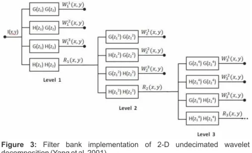
Figure 3 shows the filter bank implementation of a 3-level 2-D undecimated wavelet transform (Yang et al., 2002). H(z) and G(z) denote the z-transform of the low-pass filter h[n] and the high-pass filter g[n] respectively. I(x,y) denotes an image and (x,y) the spatial indices.
Figure 3: Filter bank implementation of 2-D undecimated wavelet decomposition (Yang et al. 2001)
1 2 3
{W (x,y), W (x,y), W (x,y)}r r r denotes the wavelet coefficients at scale r (detail subimages) with diagonal, horizontal and vertical orientation respectively.
{R (x,y)}r represents the residue signal at scale r (approximation subimage). Compared to the critically sampled wavelet transform, the undecimated wavelet transform achieves translation invariance, a desirable feature for pattern recognition applications such as fabric defect detection.
In our experiment, the fabric image was divided into non-overlapping windows of size 32x32 pixels and each window is classified as defective or defect-free. The features used to characterise each window are the channel variances at the output of the wavelet decomposition as described by the equation (5).
We used 3 levels of wavelet decomposition, and therefore the feature vector to characterise each window comprised 9 features, as shown by equation (6).
Yang et al. (2002) report that channel variances are able to provide efficient discriminations among different types of textures.
We used 2 types of wavelet described by the corresponding filters H and G. The first wavelet is the standard Haar wavelet, whereas the second wavelet is a custom wavelet whose filters are designed using a procedure which performs a cascade-form factorization for [H(z), G(z)] as reported by Yang et al. (2001) This is done using equation (7).
Structurally, this design satisfies the power complementary constraints on filter H(z) and G(z) as given by equation (9).
Another constraint on those wavelet filters is given by equations (10) .
Yang (2003)
(5)
This constraint is met when the cascade-form factorization parameters comply with the equations (11) or (12).
where m is the order of the wavelet filter H(z).
3. CLASSIFIERS
The experiments were performed using three different classifiers
• The Euclidean distance classifier with maximum likelihood (ML)
training
The Euclidean distance with minimum classification error (MCE) training
The feedforward neural network classifier
3.1 Euclidean distance classifiers
For an Euclidean distance classifier, each pattern class ω is characterised by j
a vector m that is the mean vector of the features of the patterns of that class j
that are members of the training set as described by equation (13). •
•
where N is the number of training pattern vectors for class ω and the j j
summation is taken over these vectors.
Determining the class membership of an unknown pattern with feature vector x requires computing the distance measures given by equation (14)
where W is the number of classes and assigning x to the class ω if Di is the i
smallest distance.
The above described procedure of training the Euclidean distance classifier, whereby for each pattern class a characteristic feature vector is the mean
vector of the corresponding feature vectors in the training set, is called “maximum likelihood training” or ML training (Yang, 2003).
The “Minimum Classification Error” (MCE) training of the classifier provides a better way of obtaining the classifier characteristic feature vectors of different
pattern classes . The algorithm starts with the characteristic
feature vectors obtained by the ML method and then adjusts them adaptively in order to achieve the highest classification rate of the feature vectors in the training set.
3.2 Feedforward neural network classifier
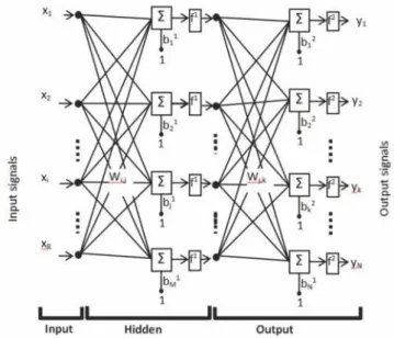
Figure 4 shows the architecture of a feedforward neural network classifier with one hidden layer.
(Yang, 2003)
Figure 4: Feedforward neural network with R inputs, M neurons in the hidden layer and N outputs (Beale et al., 2011)
The output of each neuron is computed taking the sum of the weighted inputs and the biases and passing it through the transfer function. The transfer function is typically a sigmoid function.
Among the algorithms used for supervised training, the backpropagation has emerged as the most widely used and successful for image processing (Chi, 2004). During the training phase, the feature vectors of the training set are presented at the inputs of the network and the resulting outputs are compared
Then, using a gradient descent optimization algorithm, the weights and the biases of the network are adjusted to minimise the mean square error between the network outputs and the desired outputs.
Once trained, the network can be used to give reasonable answers when presented with inputs that the network has never seen.
4. EXPERIMENTS
We performed the experiments using fabric images from the TILDA dataset . This dataset contains images of four different classes of fabrics:
• Class 1: Very fine fabrics with or without visible internal structure.
Class 2: Fabrics with a low variance stochastic structure. The surface of this class contains no imprints.
Class 3: Fabrics with a clearly visible periodic structure. Class 4: Printed materials with no apparent periodicity.
Figure 5 shows samples of the four fabric classes contained in the dataset. •
• •
Figure 5: Samples of the 4 fabric classes contained in the TILDA dataset. From left to right class 1, class 2, class 3 and class 4.
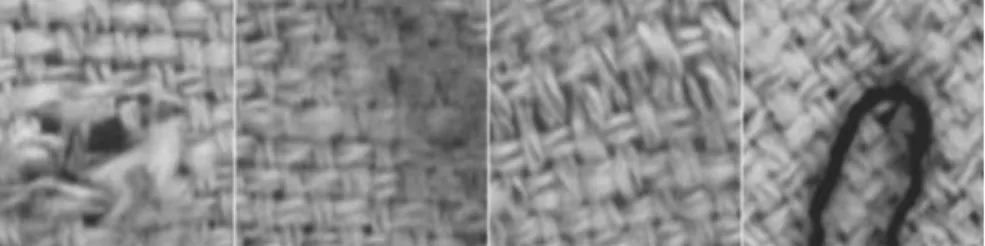
We considered fabric images with four types of defects; holes and cuts; oil stains and colour fading; thread errors; and finally foreign body on the fabric. Figure 6 shows examples of these defect types in the fabric of class 2.
Figure 6: Examples of the 4 types of defects considered in this paper. From left to right hole or cut, oil stain, thread error and foreign body.
The experimental samples were made up of image patches extracted from the fabric images as follows. Each fabric image was divided into non-overlapping windows of size 32x32 pixels. All the 37546 defective windows contained in the dataset were used in our experiments. Then 37546 defect-free windows were chosen randomly to complete the experimental dataset. From each fabric image, the same number of defect-free windows as defective windows was chosen. Half of the defective samples and half of defect-free samples were used as training set while the remaining samples were used as testing set.
From each window, five sets of features were extracted and then used separately in different experiments:
Set 1: 28 GLCM features computed as follows. Four co-occurrence matrices
o o
were computed for the inter-pixel distance d=1 pixel and for angles θ=0 , 45 ,
o o
90 and 135 . Then the 14 Haralick features (Haralick et al., 1973) were extracted from each co-occurrence matrix and finally the 14 averages and the 14 ranges of those features from the 4 matrices were used to make up the feature set.
Set 2 and Set 3: Features extracted according to the Gaussian Markov Random Field (GMRF) model. They were the model parameters of the texture in the window of interest of the fabric image. They were calculated using the least square error estimation (Al-Kadi, 2008). Set 2 comprised 6 features obtained using a model on a 3x3 neighbourhood while Set 3 comprised 14 features obtained using a model on a 5x5 neighbourhood.
Set 4 and Set 5: Wavelet features extracted as follows. A three-level undecimated wavelet transform was performed on the whole image fabric containing the window of interest. Then the means of squares of wavelet coefficients of the corresponding 32x32 windows of the detail sub-images were calculated. As a 3-level wavelet transform produces nine detail sub-images, nine features were obtained. Set 4 was obtained by using the standard Haar wavelet, while Set 5 was obtained using a custom wavelet. All the features were normalized to fit into the range [0, 1] for the samples of the training set. The features of the samples of the testing set were also normalized using the same scaling parameters as used for the training set before being used for classification purpose.
For each feature set, three different classifiers were used; the Euclidean distance classifier trained using the maximum likelihood (ML) method, the Euclidean distance classifier trained using the Minimum Classification Error (MCE) method and the feedforward neural network trained using the backpropagation algorithm to minimize the minimum square error (MSE).
5. RESULTS AND INTERPRETATION
The chart in Figure 7 shows the average detection performance of the three detection methods when the three different classifiers were used. Such performance was obtained for all the samples in the dataset. It can be seen that GLCM feature-based method performed much better than the wavelet feature-based method (using both the standard Haar wavelet and the custom wavelet) and the MRF feature-based methods. The difference in the detection rates is significant. It can be seen from the results that when the MCE-trained Euclidean distance classifier is used, the difference between the detection rate yielded from the GLCM feature-based method and the best wavelet feature-based method is 7.9%. The difference is 2.0% when the ML-trained Euclidean distance classifier is used and 12.1% when the neural network classifier is used. The trends of detection performance among the three detection methods we used seem to be classifier-independent as these are consistently seen among the three classifiers used in our experiments.
The chart in Figure 7 also shows that the wavelet feature-based method performed better than the MRF feature-based method. However, the difference of defect detection performance of wavelet feature-based method with respect to the MRF feature-based method is much smaller than the one displayed by GLCM feature-based method compared to the two other methods. For example, when the MCE-trained Euclidean distance classifier was used, the GLCM feature-based methods yielded a detection rate of 7.9% higher than the detection rate obtained by the best wavelet-based features, while the best wavelet-based method yielded merely a detection rate of only 2.6% higher than the best MRF feature-based method.
From the observations above, we can conclude that GLCM features discriminate fabric texture more than channel variances of sub-images of the undecimated wavelet transform. Likewise, we can conclude that channel variances of the sub-images of the undecimated wavelet transform are more discriminative than GMRF model parameters of the same fabric texture.
Figure 7: Average detection rate with different types of features and different classifiers
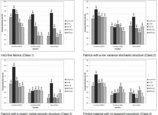
Looking at the defect detection performance for different types of fabrics as shown in the charts of Figure 8, one can see that the general trend observed in previous paragraphs was generally maintained for individual fabric types. The exception to the general trend is observed for printed materials with no apparent periodicity (Class 4) and partly for fabrics with a clearly visible periodic structure (Class 3). It is observed that for printed materials with no apparent periodicity (Class 4), MRF features - especially on a 3x3 neighbourhood - performed better than wavelet features.
In all cases, the Euclidean distance classifier with MCE training performed better than the other classifiers considered. Also, all the detection methods performed better on very fine fabrics (Class 1) and performed worst on printed materials with no apparent periodicity (Class 4). This happens because the texture on very fine fabrics is more uniform than on the others types of fabrics considered. In contrast, the texture on printed material with no apparent periodicity seems less uniform than on the other types of fabrics.
Figure 8: Defect detection performance for different types of fabrics
6. CONCLUSIONS
Table 1: Average detection performance for different detection methods and different classifiers.
Feature extraction method
GLC M MRF UDWT 3x3 neighbourhood 5x5 neighbourhood Custom wavelet Haar wavelet Classifier Euclidean (MCE) 82.2% 71.7% 69.5% 72.7% 74.3% Euclidean (ML) 69.3% 65.0% 63.0% 67.3% 66.6% Neural network 73.4% 59.5% 60.5% 61.3% 61.3%
In this paper, we compared the performance of three methods of fabric defect detection. As summarised in Table 1, we have found that, generally, the GLCM feature-based method performed better defect detection than wavelet feature-based methods, while the wavelet feature-based methods generally allowed better detection than MRF feature-based methods.
This general trend does not seem to apply to fabrics with no apparent periodicity where the MRF feature-based method performs better than the wavelet feature-based method.
We have also found that the considered methods performed better on fabrics with uniform texture than on fabrics where texture has less uniformity. Finally, we have found that the Euclidean distance classifier with minimum classification error (MCE) training performed better than both the Euclidean distance classifier with maximum likelihood (ML) training and the feedforward neural network classifier with back-propagation training.
7. REFERENCES
Al-Kadi, O. S. (2008) Combined statistical and model based texture features for improved image classification. In Advances in Medical, Signal and Information Processing, 2008. MEDSIP 2008. 4th IET International Conference on, pp. 1-4.
Beale, M. H., Hagan, M. T., and Demuth, H. B. (2011) Neural Network
TM
Toolbox : User's Guide, The MathWorks, Inc.
Bodnarova, A., Bennamoun, M., and Kubik., K. K. (2000) Suitability analysis of techniques for flaw detection in textiles using texture analysis. Pattern Analysis & Applications, 3, pp. 254-266.
Chi, L. T. (2004) Fabric Defect Detection by Wavelet Transform and Neural Network. Master's Thesis, University of Hong Kong.
Cohen, F.S., Fan, Z., and S. Attali (1991) Automated inspection of textile fabrics using textural models. IEEE Trans. PAMI vol. 13, pp. 803–808.
Conners, R.W., and Harlow , C. A. (1980) A theoretical comparison of texture algorithms. IEEE Transactions on Pattern Analysis and Machine Intelligence, 3, pp. 204-222.
Haralick, R.M., Shanmugam, K., and Dinstein, L. (1973) Textural features for image classification. IEEE Trans. Syst., Man., Cybern., vol. SMC-3, pp. 610-621.
Kumar A. (2008) Computer-Vision-Based Fabric Defect Detection: A Survey. IEEE Transactions on Industrial Electronics, pp. 348-363.
Miyamoto, E. , and Merryman, T. (2005) Fast calculation of Haralick texture features. [Online] [Accessed Feb 2011]. Available at:ce.cmu.edu/~pueschel /teaching/18799BCMUspring05/material/eizantad.pdf.
Ngan, H. Y., Pang, G. K., and Yung, N. H. (2011) Automated fabric defect detection—A review. Image and Vision Computing, 29(7), pp. 442-458.
Technical University Hamburg-Harburg, Technical Information Technology (1996) A reference dataset for evaluation of visual inspection procedure for textile. Internal Report.
Weszka, J.S., Dyer, C. R., and Rosenfeld, A. (1976) A comparative study of texture measures for terrain classification. IEEE Transactions on Systems, Man and Cybernetics, 4, pp. 269-285.
Yang, X. Z., Pang, G. K. H., and Yung, N.H.C (2001) Fabric Defect Detection Using Adaptive Wavelet. Proc. ICASSP-2001, vol.6, pp. 3697-3700.
Yang, X. Z., Pang, G. K. H., and Yung, N.H.C. (2002) Fabric Defect Classification Using Wavelet Frames and Minimum Classification Error Training. IEEE 2002 37th IAS Industry Applications Conference Meetings, vol.1, pp. 290–296.
Yang, X. Z. (2003) Discriminative Fabric Defect Detection and Classification Using Adaptive Wavelet. Ph. D. Thesis, University of Hong Kong