Abusive and Hate Speech Tweets Detection with Text Generation

(1)

Wright State University Wright State University

CORE Scholar

Browse all Theses and Dissertations Theses and Dissertations

2019

Abusive and Hate Speech Tweets Detection with Text Generation

Abhishek Nalamothu

Wright State University

Follow this and additional works at: https://corescholar.libraries.wright.edu/etd_all

Part of the Computer Engineering Commons, and the Computer Sciences Commons

Repository Citation Repository Citation

Nalamothu, Abhishek, "Abusive and Hate Speech Tweets Detection with Text Generation" (2019). Browse all Theses and Dissertations. 2094.

https://corescholar.libraries.wright.edu/etd_all/2094

This Thesis is brought to you for free and open access by the Theses and Dissertations at CORE Scholar. It has been accepted for inclusion in Browse all Theses and Dissertations by an authorized administrator of CORE Scholar. For more information, please contact [email protected].

(2)

ABUSIVE AND HATE SPEECH TWEETS

DETECTION WITH TEXT GENERATION

A Thesis submitted in partial fulfillment

of the requirements for the degree of

Master of Science

by

ABHISHEK NALAMOTHU

B.E., Saveetha School of Engineering, Saveetha University, India, 2016

2019

(3)

Wright State University GRADUATE SCHOOL

June 25, 2019 I HEREBY RECOMMEND THAT THE THESIS PREPARED UNDER MY SUPER-VISION BY Abhishek Nalamothu ENTITLED Abusive and Hate Speech Tweets Detection with Text Generation BE ACCEPTED IN PARTIAL FULFILLMENT OF THE REQUIRE-MENTS FOR THE DEGREE OF Master of Science.

Amit Sheth, Ph.D. Thesis Director

Mateen M. Rizki, Ph.D. Chair, Department of Computer Science and Engineering Committee on Final Examination Amit Sheth, Ph.D. Keke Chen, Ph.D. Valerie L. Shalin, Ph.D. Barry Milligan, Ph.D.

(4)

ABSTRACT

Nalamothu, Abhishek. M.S., Department of Computer Science and Engineering, Wright State Uni-versity, 2019.Abusive and Hate Speech Tweets Detection with Text Generation.

According to a Pew Research study, 41%of Americans have personally experienced online harassment and two-thirds of Americans have witnessed harassment in 2017. Hence, online harassment detection is vital for securing and sustaining the popularity and viability of online social networks. Machine learning techniques play a crucial role in automatic harassment detection. One of the challenges of using supervised approaches is training data imbalance. Existing text generation techniques can help augment the training data, but they are still inadequate and ineffective. This research explores the role of domain-specific knowledge to complement the limited training data available for training a text generator.

We conduct domain-specific text generation by combining inverse reinforcement learn-ing (IRL) with domain-specific knowledge. Our approach includes two adversarial nets, a text generator and a Reward Approximator (RA). The objective of the text generator is to generate domain-specific text that is hard to discriminate from real-world domain-specific text. The objective of the reward approximator is to discriminate the generated domain-specific text from real-world text. During adversarial training, the generator and the RA play a mini-max game and try to arrive at a win-win state. Ultimately, augmenting diver-sified and semantically meaningful, generated domain-specific data to the existing dataset improves detection of domain-specific text. In addition to developing the Generative Ad-versarial Network-based framework, we also present a novel evaluation that uses variants of the BLEU metric to measure the diversity of generated text; uses perplexity and cosine similarity to measure the quality of the generated text. Experimental results show that the proposed framework outperforms a previous baseline (IRL without domain knowledge) on harassment (i.e., Abusive and Hate speech) tweet generation. Additionally, the generated tweets effectively augment the training data for online abusive and hate speech detection

(5)

(tweet classification) resulting in a 9% accuracy improvement in classification using the augmented training set compared to the existing training set.

(6)

List of Figures

2.1 Example of a size 5 window . . . 7

2.2 The Skip-Gram model architecture . . . 8

2.3 Mapping word embeddings with Word2vec . . . 10

2.4 The basic idea of reinforcement learning and elements involved in it . . . . 13

2.5 Reinforcement learning demonstration with Maze Game Environment . . . 15

2.6 Feeding pong game frames to a policy network. . . 18

2.7 Value based RL approach on Grid game. . . 19

2.8 Sparse Reward failure of RL algorithm . . . 20

2.9 Decision boundary of an SVM classifier with separating hyper-planes on both sides. . . 22

3.1 State of the art Text generation models . . . 24

3.2 Recurrent neural network-folded form. . . 25

3.3 Recurrent neural network - unfolded form . . . 26

3.4 The left plot represents Cross entropy vs Cost function. The right plot represents the objective i.e., Minimizing the cost. . . 29

3.5 Recurrent neural network - training with example . . . 30

3.6 A recurrent neural network with one hot encoded targets . . . 30

3.7 A recurrent neural network - Back Propagation through time . . . 33

3.8 A recurrent neural network - Long term dependency problem. . . 34

3.9 Sigmoid f(x) and it’s derivative ∂f_∂x . . . 37

3.10 Tanh f(x) and it’s derivative ∂f_∂x . . . 38

3.11 Recurrent Neural network - Vanishing Gradient problem . . . 39

3.12 Recurrent Neural network - Exploding Gradient problem . . . 40

3.13 Gradient clipping . . . 41

3.14 ReLU activation functionf(x)and it’s derivative ∂f_∂x . . . 42

3.15 Standard Vanilla RNNs. . . 43

3.16 LSTM . . . 43

3.17 Notations used in the LSTM. . . 44

3.18 LSTM - Memory (cell) value propagation . . . 44

3.19 Working Mechanism of LSTM with example. . . 45

3.20 LSTM - Forget fate (ft₎ _{. . . 46}

(9)

3.22 LSTM - updating its cell state . . . 47

3.23 LSTM - output gate . . . 48

3.24 A recurrent neural network - Text generation . . . 49

3.25 Generative Adversarial networks - image generation. . . 51

3.26 The illustration of SeqGAN. Left: Discrimator training. Right: Generator training [32] . . . 58

3.27 Rank GAN . . . 60

4.1 MCMC sampling at each state for computing the expected total reward using Reward approximator R . . . 67

4.2 Our method architecture . . . 72

5.1 Proportion of harassment tweets and non- harassment tweets . . . 76

5.2 Data set division. . . 76

5.3 Data Pre-processing . . . 77

5.4 Pipeline of our framework . . . 78

7.1 Generator objective plot. . . 87

(10)

List of Tables

3.1 Passing of memory value through the chain of repeated layers. . . 44

3.2 Objective of the generatorGand the discriminatorD . . . 51

5.1 Example tweets from each class . . . 75

5.2 Hyper-parameters configurations.. . . 77

6.1 BLEU example . . . 79

6.2 BLEU score calculation for candidate w.r.t reference sentence (example from the above table) . . . 80

6.3 Configuration ofBLEUdiv andBLEUs . . . 80

6.4 Experimental results between IRL (previous base line) andIRLcs(our model) 82 6.5 Experimental results of MCS . . . 83

7.1 Examples from training data, and generated data from different techniques . 84 7.2 SVM classification results on different techniques . . . 86

(11)

Acknowledgment

Guru (Teacher) = ”GU” means darkness, ”RU” means dispeller. Thanks to all my Gurus (Advisor and committee).

Firstly, I would like to express my sincere gratitude to my thesis advisor Dr. Amit P. Sheth for his continuous support, patience, motivation, and immense knowledge. His guidance helped me in all the time of research. I could not have imagined having a better advisor for my thesis study.

Also, I would like to convey my sincere gratitude to the rest of my thesis committee: Dr. Keke Chen, Dr. Valerie L. Shalin, and Dr. Krishnaprasad Thirunarayan, for their insightful comments and encouragement, and for the hard question which incented me to widen my research from various perspectives.

My sincere thanks also goes to my mentor Dr. Shreyansh Bhatt for believing in me and always giving me the right push.

I would also like to thank everyone at Kno.e.sis to make my time here enjoyable and mem-orable.

Finally, I must express my very profound gratitude to my parents and my family for letting me pursue my dreams. I could not have asked for anything better. I wouldn’t be here with-out your love and support.

(12)

Dedicated to my father Sri Hari Nalamothu (1963-2008). Thank you for always watching over me and your guiding hand will forever be on my shoulder.

(13)

1

Introduction

Online social media such as Twitter and Facebook are vital communication and networking mediums. According to a Pew Research study, approximately 76%of the American popu-lation used social media in 2017, compared to just 7%in 2005 [24]. With the popularity of social network among school and college studnets [6], it is important to detect attempts of potential online harassment.

Machine learning techniques play a crucial role in automatic harassment detection. Based on our analysis of online content, we found that the amount of truly harassing social media content relative to normal content is small, but it can have serious consequences on a victim. So while this is a significant problem, it is also challenging to develop automatic harassment detection system based on supervised learning. Therefore, augmenting training with an improved harassment training data can improve harassment detection. Existing text generation techniques based on Generative Adversarial Networks (GANs) provide a novel approach to augmenting the training data. In this thesis, we focused on detecting a particular form of online harassment i.e., abusive and hate speech detection.

Coherent and semantically meaningful text generation that mimics the real world text is a crucial task in NLP (Natural Language Processing). Recent studies have shown that auto-regressive models such as recurrent neural networks (RNNs) with the Long Short

(14)

Term Memory networks (LSTMs) [10, 29, 31] can achieve excellent text generation per-formance. However, they suffer from an exposure bias problem [1], i.e., generator can see the previous token while training but do not have an access to it while generating the text samples. Current proposed techniques to solve this problem include Gibbs sampling [28], scheduled sampling [1], and adversarial methods, such as SeqGAN [32], LeakGAN [11], MaliGAN [4], and RankGAN [17]. GAN techniques have been the most popular tech-niques as they do not require to define an explicit probability density function[9]. In GAN, a discriminator helps adversarial text generation models to evaluate whether a given text is real or not. Then a generator aims to generate text that is hard to discriminate from the real-world text, which results in a maximized reward signal from discriminator via reinforce-ment learning (RL). The entire text sequence generation of these adversarial techniques can alleviate the problem of exposure bias. In spite of their success, these adversarial models still face two challenges such as reward sparsity and mode collapse.

Diverse text generation by employing inverse reinforcement learning (IRL) [27] is proposed to tackle these two challenges. This model assigns instant rewards to a gener-ation policy that generates text sequence by sampling one word at a time, thus providing dense reward signals. Using an entropy regularized policy gradient [7] as an optimization policy results in a more diversified text generator. Both dense rewards and entropy regu-larized policy gradient can alleviate reward sparsity and mode collapse (It happens when the generator learns how to produce samples from a few modes of the data distribution still misses many other modes i.e., the generator generates a limited diversity of samples, or even the same sample, regardless of the input). However, this model suffers with a small training data set because deep adversarial neural nets have high model capacity and depend on the availability of large quantities of the training data to learn a nonlinear function that generalizes the distribution.

To address the data scarcity challenge, we propose a framework that incorporates domain-specific knowledge into the IRL-based text generation model. Using IRL with

(15)

domain-specific knowledge, we show that maximization of cosine similarity between gen-erated sentence Word2Vec (W2V) embedding and training data W2V in an optimization policy will lead to better text generation with less training data. Here, W2V embeddings are modeled using domain-specific knowledge (tweets). In addition to the framework, we present a new evaluation that uses metrics including variants of BLEU [22] to measure the diversity of generated text; and perplexity and cosine similarity to measure the quality of the generated text. Variants of BLEU such as Diverse BLEU and Self BLEU measure diversity between generated data and training data, and the generated data to itself respectively. For any given text generation model, perplexity measures how well a model predicts a sample text. Cosine similarity between generated sentence W2V and training W2V measures the quality of the generated text. Experimental results on these metrics show that the proposed framework outperforms the previous baseline (IRL without domain knowledge) on abusive and hate speech tweet generation. Ultimately, the generated tweets effectively augment the training data for online abusive and hate speech detection (tweet classification) resulting in a9%improvement in classification accuracy with the augmented training set compared to the existing training set.

The contributions of this work are summarized as follows:

1. We extend the optimization of IRL-based GAN to incorporate a domain knowledge term that preserves meaning so as to generate diverse and meaningful text given a small training data set.

2. We propose three new evaluation measures based on the BLEU score, perplexity, and cosine similarity to better evaluate the quality and diversity of generated texts. 3. We enhanced the detection of abusive and hate speech tweets by providing generated

(16)

Chapter Overview

The rest of the thesis is organized as follows.

Chapter 2: Preliminaries Contains essential definitions (that are required to understand

our work) with examples to provide an overview of Word2Vec, Language Modeling (LM), Reinforcement Learning (RL), Inverse Reinforcement Learning (IRL), and Support Vector Machine (SVM) classification.

Chapter 3: Related Work Reviews earlier attempts to generate text. In this chapter, we

talk about problems with existing algorithms.

Chapter 4: Research Contribution to Text Generation Explains intuition behind how

adding a domain knowledge term to the latest text generation optimization function produce better sentences given a small training dataset.

Chapter 5: Data & Experimental setting Describes the abusive and hate speech tweet

dataset. Also, it presents the optimal hyper-parameter setting and pipeline for our experi-ment.

Chapter 6: Evaluation Illustrate the necessity for new evaluation metrics. Explains how

proposed new measures capture the diversity and quality of generated sentences.

Chapter 7: Results & Conclusion Compares examples of generated sentences and the

classification results of our technique with others. Also, we talk about future improvements and concludes our thesis work.

(17)

2

Preliminaries

This chapter helps the reader to understand the background knowledge that is expected to study the thesis work presented in the following chapters. We discuss the following topics:

1. The Skip-Gram (SG) word2vec model 2. Language Modelling (LM)

3. Reinforcement Learning (RL)

4. Inverse Reinforcement Learning (IRL)

5. The Support Vector Machine (SVM) binary classifier

2.1

Word2vec

The combination of Natural Language Processing (NLP), and Artificial intelligence (AI) allows machines to process human language and, in some scenarios, even repeat it. The end goal of NLP is to understand and interpret meaning in a way that is helpful for a human user. But, understanding is one of the primary challenges of NLP. This is because machines use binary, unlike text and speech used by humans. NLP needs a process that transforms

(18)

text and speech to numbers. This process is called word embedding, with Word2Vec as one of the more well-known embedding models.

Word2Vec (a prediction based model) was introduced by Tomas Mikolov et al., 2013 [20] (a Czech computer scientist working in the field of machine learning) at Google. It is a semantic learning framework that utilizes a two-layer neural network to learn the vector representation of words or phrases in a particular corpus. The Word2Vec model takes text as input and outputs feature vectors that represent the vocabulary of a corpus. This model utilizes predictive analysis to guess a word based on its neighboring words, unlike frequency-based models. The 2 variants of the Word2Vec model are:

1. Continuous Bag of Words (CBOW): This model learns to maximize the probability

of a target word based on its neighboring words (a window of words around the current word). Thus the model learns to guess the words by looking at its context. Therefore, it learns to generalize the way the word can be used in all distinct contexts. This type of learning gives less attention to rare words because the objective is to guess the most probable words.

For example,it is really a ... day to go to a picnic. In this instance, the model tries to predict “beautiful” rather than “delightful” because of word probabilities. This makes the model unable to learn infrequent words.

2. Skip-Gram (SG): This model learns to predict the neighboring words (context)

based on the current word. So, in the example case, the model takes “delightful” and guesses its context i.e.,it is really a ... day to go to a picnicwith high proba-bility. This model gives equal attention to both infrequent and frequent words. Here, the combination of “delightful” and its neighboring words is treated as a new obser-vation. Therefore, this model needs sufficient samples for each context.

According to Mikolov, SG works well with a small training corpus, and even learns and represents rare words effectively. So, we choose this Skip-Gram model to train word

(19)

embedding because we also have limited training data. Let us now look into the details of the Skip-Gram model.

2.1.1

Skip-Gram model Learning Objective

The objective of the SG model is to create a word embedding that is effective for predicting the neighboring words given a current word. Specifically, the model tries to maximize average log-likelihood throughout the entire corpus.

argmaxø 1 T T X t=1 X j∈n,j6=0 logp(wt+j|wt; ø) (2.1)

This equation states that there is some likelihoodpto observe a specific word within a size n window of the present word wt. The probability of the neighboring words is

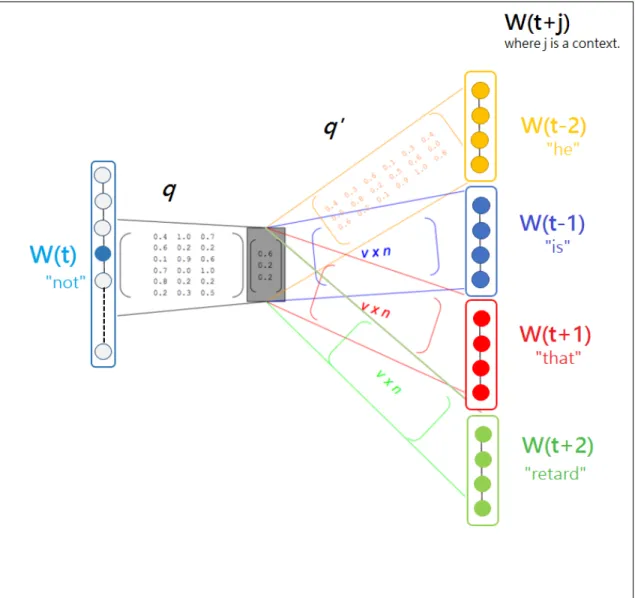
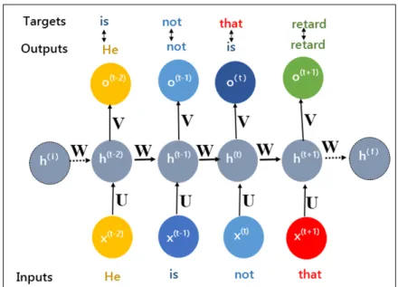
conditioned on wt and the setting of parameterø. For example, the probabilities of the

words “he”, “is”, “that”, “retard” depends on the current word “not” as shown in Figure

2.1and a model parameterø. The model optimizesøso that the conditional probability of neighboring words is maximized throughout the entire corpus.

Figure 2.1: Example of a size 5 window

In Figure 2.1, the current word wt is “not”, and neighboring words are “He”, “is”,

“that”, “retard”

2.1.2

Skip-Gram model architecture

The Skip-Gram model architecture is a two-layer neural network. It uses a linear activation function in hidden layers and the Softmax activation function in the output layer. It is not

(20)

possible to directly feed the text to a neural network. One of the effective ways to feed text input is to convert all of the words from a corpus vocabulary into one-hot encoding vectors(A one-hot vector is a1×N matrix (vector) used in natural language processing to differentiate each word in vocabulary from any other word in the vocabulary. The vec-tor comprises of zeros in all positions with the exception of a single 1 in a position used uniquely to identify the word). For example, “he” is theithword in the corpus vocabulary. So, a one-hot encoding vector that represents “he” contains 1 at ith _{position and 0 at all}

other positions.

(21)

Figure2.2shows the Skip-Gram model two-layer neural network architecture. It uses a linear activation function in the hidden layers and Softmax activation function in the output layer. q andq0 are the weights which are represented by the parameter ø. j is the context.

Hidden layer

A hidden layer utilizes linear activation functions. A weight matrix withkrows ( where

kis the size of the vocabulary) andlcolumns (wherelis size of the features that SG model extracts from each sample) represents the hidden layer. The hidden layer is computed by doing matrix multiplication between a k-dimensional one-hot encoded vector and a k×l

weight matrixq. The matrix row corresponding to “1”(in the one-hot encoded vector) will be selected as shown in the following matrix multiplication.

0 0 1 ... 0 ×             z11 z12 z13 ... z1l z21 z22 z23 ... z2l z31 z32 z33 ... z3l ... ... ... ... ... zk1 zk2 zk3 ... zkl             = z31 z32 z33 ... z3l

This implies that the hidden layer only works as a look-up table. The resulting hidden layer output represents a word vector for a given word input.

Output layer

The resulting word vector of dimension1×l from matrix multiplication is given to the output layer. The output layer utilizes a Softmax activation function. The output layer consists of n number (window size) k-dimensional vectors as shown in Figure 2.2. The outputs (probabilities) of these eachk-dimensional vector vary from 0 to 1 and their sum is equal to 1. For example, consider the architecture as shown in Figure2.2with vocabulary

(22)

size as 5.

output vectorw(t+1) = [He, is, not, that, retard]

= [0.16,0.12,0.02,0.55,0.15] =that

Similarly, the model applies softmax on the remaining three 5-dimensional vectors, where it ideally aims to output “He”, “is”, and “retard”.

Intuition

If two distinct words have similar neighboring words (context), then the model outputs very similar word embeddings for these two words. Thus, given current words, the model outputs very similar neighboring words. For example, the model outputs similar neighbor-ing words for the input words “Boy” and “girl”. This is because their word embeddneighbor-ing vectors are closer to each other. Consequently, word embeddings help machines to capture the semantics of natural human language.

Figure 2.3: Mapping word embeddings with Word2vec

(23)

“boy” and “Rome” because the likeness of boy and girl appearing in a similar context is high.

2.2

Language Modeling (LM)

Language modeling (LM) informs many kinds of Natural language processing (NLP) appli-cations, such as Sentiment analysis, Question answering, Machine translation, Text gener-ation, speech recognition, and summarizgener-ation, etc. The responsibility of LM is to represent the text in an accessible form for a computer. The problem with language modeling is that natural language vocabulary introduces ambiguity that human beings readily resolve. Us-ing conventional grammar and structure, lUs-inguists attempt to define language with brittle success. Learning from the data is an alternative approach to model language. There are two approaches to model the language from data.

1. Statistical Language Models: A statistical language model is a probability

distri-bution over word sequences. It assigns probabilityp(w1, w2, ..., wT) to a sequence

of tokens i.e., from a sentence in a language. In other words, it is the likelihood of seeing a sentence in the corpus. For example:

p1 =P(“Tomorrow is going to be sunny00) = 0.01 p2 =P(“Tomorrow is not good for a rocket launch00) = 0.00001

While both examples are valid sequences, probability of sequence 1 is high because, for instance, the LM can better model general weather discussions rather than the favorable weather for a rocket launch given a weather corpus. In addition to assigning a probability to each sequence, LM also assigns the probability of a given word following the sequence. That is, LM learns to predict the next word given the true sequence.

(24)

2. Neural Language Models: Thecurse of dimensionalityis a basic issue that makes language modeling and other learning issues hard. The dimensionality curse occurs when a vast amount of distinct word combinations from vocabulary need to be dis-criminated, and the learning algorithm requires at least one instance per appropriate word combination. The number of necessary examples may expand exponentially as the amount of vocabulary rises. In language modeling, the issue arises from the enor-mous amount of possible word sequences. For example, with a series of 10 words taken from a104 _vocabulary,₁₀50_{possible sequences are available.}

Neural Language Modeling (NLM) exploits an ability to generalize distributed rep-resentations to diminish the impact of the dimensionality curse. The NLM learns to map word embedding vectors (features vectors) to a prediction of interest, such as computing the probability distribution of a target word given the true sequence. A word embedding vector (Word2Vec) enables words with a similar meaning to have closer representations based on their use. When two word embeddings are closer to each other, then they are functionally similar (semantic and grammatical similarity) and can be replaced in the same context by one another, helping the neural network to model a function that makes good predictions about the training set (that is, the set of word sequences from a corpus used to train the model).

Bengio et al., (2003) [2] described NLM with the following 3 model properties:

(a) Maps each word in the vocabulary to a word embedding (a vector which cap-tures feacap-tures of words)

(b) Expresses the joint probability function of word sequences in terms of their word embedding.

(c) Learns the word embedding and the probability model parameters at the same time.

(25)

and probability function that represents a model from the training corpus.

The neural-network-based language modeling approaches have recently begun to con-sistently outperform the classical statistical modeling methods, both as standalone applica-tions and as a part of more difficult NLP applicaapplica-tions.

Initially, feed forward neural networks are used to model language. Later, Recurrent Neural Networks (RNNs) and Long Short Term Memory (LSTM), a special kind of RNNs, are introduced to model the language for longer sequences (Next chapter3discusses details of RNNs and LSTM.).

2.3

Reinforcement Learning (RL)

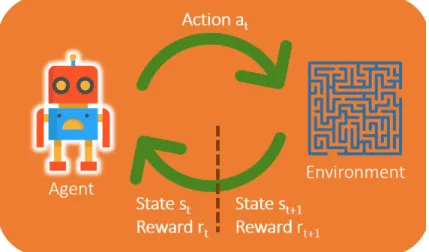
Reinforcement learning (RL) is a form of machine learning. It allows an agent to make a sequence of decisions using feedback from its actions and experiences through trial and error in an interactive environment to maximize some notion of collective reward. RL is utilized by various machines and software to discover an optimized path or behavior for a specific scenario.

(26)

Key terminology of Reinforcement learning:

In Figure2.4, the agent performs actionatgiven statest, and rewardrt(for the previous

action). According to the actionat, the environment provides rewardrt+1 and statest+1to

the agent This is an iterative process until agent reaches the final state.

1. Environment: Physical/Digital world where the agent works.

2. State: The agent’s current situation in the Environment.

3. Reward: The environment’s feedback.

4. Policy: Model(probability function) that maps the state of the agent to its actions.

5. Value: Future reward that an agent would collect by executing an action in a specific

state.

Comparison of RL with supervised and unsupervised learning

Although both RL and supervised learning use mapping between input and output, they differ. Unlike supervised learning, which uses target label to provide a correct set of actions to the agent as feedback for performing a task, RL utilizes rewards and penalty as signals of beneficial and negative behavior. In other words, training data in supervised learning comes with an answer key, so that the model is trained with right answers. While there is no answer key in reinforcement learning, reinforcement agents choose what actions to perform to accomplish the given task. It is bound to learn from its experience despite the lack of a training dataset. RL can best be clarified through games, such as the maze below. In supervised learning training data appear as follows:

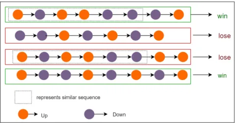
1. l,r,u,r,d,l,d,u,r,l−→w 2. l,l,r,u,d,r,l,r,u,d−→lo

(27)

where l, r, u, d, w, lo corresponds to left, right, up, down, win, and lose respectively. Both the data samples came with labels (win/lose), which informs the agent by following this se-quence of actions, it will either win/lose. But, a reinforcement agent looks at the scoreboard (reward) given by the maze game environment as feedback to optimize its learning.

Reinforcement learning is distinct in terms of objectives compared to unsupervised learning. While the goal of unsupervised learning is to find similarities and differences between data points, the goal of reinforcement learning is to find an appropriate model of action that maximizes the agent’s total collective reward.

2.3.1

Exploration and exploitation trade off

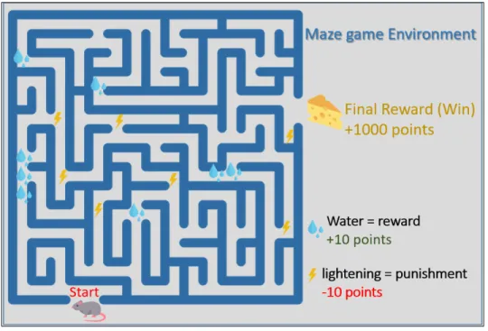
In reinforcement learning, there is a significant notion of exploration and exploitation trade-off. Exploration is about discovering more information about the environment, while ex-ploitation is profits from already known information to maximize rewards.

Figure 2.5: Reinforcement learning demonstration with Maze Game Environment

(28)

water (a smaller reward worth + 10 points) on its path. In the meantime, the robot mouse wants to avoid lightening spot (electric shock punishment worth -10 points) on its path.

The maze game example illustrates the exploration and exploitation trade-off. In this example, the robot-mouse wants to reach the endpoint where it gets cheese as the final reward. In this game, after some exploration, the mouse could discover the three sources of water grouped near the entrance and may waste all of its time exploiting this discovery of mini-paradise. By continuously exploiting this discovery, the mouse earns small rewards and never proceeds into the maze to seek a bigger reward. This scenario illustrates the significance of the trade-off between exploration and exploitation. A simple approach for the mouse would be executing the best-known actions (which surely provides rewards) for most (say 75-80%) of the times, while exploring a fresh, randomly chosen path in the remaining (say 20-25%)times, although wandering away from the known prize.

This approach is called an epsilon-greedy approach, where epsilon decides the per-centage of time an agent explores a randomly chosen path instead of performing the best-known action to maximize the rewards. In practice, people start the RL model with a high epsilon value and reduce this value after a delay. The agent (mouse) thus explores and learns about the majority of the environment over the time, discouraging further exploita-tion of known environment to encourage further exploraexploita-tion. Nevertheless, reward is not always immediate. In the maze game, the robot-mouse may traverse a lengthy stretch of the maze passing several decisions points before reaching the final reward.

2.3.2

Approaches to Reinforcement Learning

Following are the two major approaches to solve reinforcement learning problem.

1. Policy-based approach: Mathematically, we represent policy as follows:

(29)

Whereπis a policy function that maps each statesto the best corresponding actiona

(from the available actions) at that state. The policy essentially defines the behavior of the agent. π funtions as a conduct policy: “the best thing to do when I observe state s is to take action a”. For example, consider an automatic driving car policy that includes something like: “If car sees a yellow light and it is more than 100 feet from the junction, then it should apply the brake. Otherwise, continue to move forward”. The objective of the policy function is to maximize expected reward (in case of automatic driving car minimizing the accidents) by choosing the best action at a given state.

We can further divide policies into two different kinds: (a) A stochastic policyπs, formally represented as follows:

πs=p(A =a|S =s) (2.3)

This gives a probability distribution over different actions given a state.

(b) A deterministic policyπdalways returns the same actiona regardless of given

states

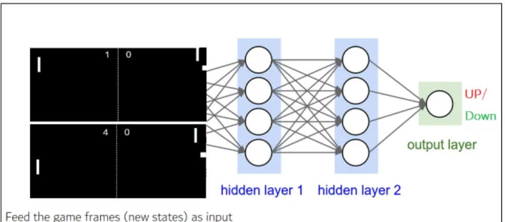
Consider an example where we teach an RL agent to play pong [16]. Here, we feed gaming frames (with the scoreboard on top) as input to the RL algorithm. The score-board in the feeding frames acts as a reward or feedback to the RL agent. Whenever the agent scores +1, the model realizes that the action taken by the policy at that state was good. So, the algorithm learns the direction in which an agent has to move depends on the scoreboard. Here we utilize deep neural networks to learn the pol-icy function. Thus, we call these a polpol-icy network (PN). PN takes frames as input and gives rewards back to the network aiming to optimize the policy using a policy gradient.

(30)

Figure 2.6: Feeding pong game frames to a policy network.

The RL agent learns to play pong in the following way. Initially, game frames are fed to the PN, letting the algorithm choose the movements of the agent. At first, movements (actions) chosen by the algorithm are bad but eventually, the agent makes a point. A set of lucky points helps the policy to understand what action to take at the given state to maximize the reward. Thus, in time, the RL agent is likely to choose those actions that give a reward compared to an action that may not. Intuitively, the RL agent is learning to play pong by optimizing the policy.

2. Value Based approach: The objective of the agent in a value-based RL approach

is to optimize the value function Vφ(s). Vφ(s)gives the maximum expected future

reward that an agent gets at each state.

Each state’s value is defined as the expected total amount of reward to be collected by the agent over the future, from a specific state.

Vφ(S) =Eφ

Rt+1+γRt+2+γ2Rt+3+..|St=s

(2.4)

WhereRt+1, Rt+2, Rt+3, ..are the rewards associated with the future states. Agent

always choose next stateswith high expected reward according toVφ(s).

(31)

Figure 2.7: Value based RL approach on Grid game.

gives the maximum expected total reward. In Figure 2.7, at each state, the value-based approach takes the largest value to achieve its goal i.e., maximum points. So, the agent follows the6→9→45→45→27→27→27path from start to end to achieve maximum rewards.

Limitation

During the training of an agent, if the agent loses points because of choosing a particular sequence of actions, then the policy model tries to discard or decrease the likelihood of choosing the same sequence of actions. This approach has a potential “sparse reward” problem as the policy model does not consider the fact that the partial sequence was useful in the training process, i.e., giving rewards at the end of the game sequence instead of giving them at each state.

In Figure2.8, except for the last 2 states, the remaining states (a good partial sequence) of sequence 3 are similar to winning sequence 1. Considering the last 2 states, the policy decreases the likelihood of a first 6 sequence of actions which may have the potential to form a winning sequence with the change of 2 last states.

The sparse reward setting of RL makes the algorithm very sample-inefficient. This requires numerous, varied training examples to train the agent. The complexity of the

(32)

Figure 2.8: Sparse Reward failure of RL algorithm

environment also contributes to the failure of sparse reward setting in many situations. Reward shaping is proposed to solve this sparse reward problem but it is limited due to the need for reward function customization for every game.

2.4

Inverse Reinforcement Learning (IRL)

In this setting, we will provide real-world data that acts as an expert agent policy or be-havior. The objective of IRL is to learn the reward function that explains expert bebe-havior. Intuitively, we assume that training data generated from the human world has the right (best) sequence of actions. Thus, learning a reward function that explains this expert’s be-havior helps the model to pick the best possible action in the future. For example, in the text generation process, estimating a reward function that explains the human written sentences supports modeling a good text generator.

Why are we interested in finding the reward function of a given problem?

In many RL tasks, there is no source for the reward signal. For example, the human-driven data feed to automate the vehicle does not have any rewards attached to it. Similarly, a human-written sentence feed to the text generation process does not have any rewards

(33)

at-tached to it. So, the data feed must be carefully hand-crafted to precisely represent the task. Usually, researchers tweak the RL agent’s reward function manually until the observation of desired behavior is reached, which is a tedious process. Therefore, IRL searches a well-suited reward function for some task by observing expert (human) performance from the training data of that task, and then automatically retrieves the respective reward function from these training data observations. Learning a reward function and then approximating the policy w.r.t a reward function is significant compared to the other way around. Also, learning a reward function captures salient features of the task whereas a policy contains many irrelevant steps to approach the task.

So, IRL better models the real-world problems given data without labeled rewards.

2.5

Support Vector Machine (SVM) Classification

SVM is one of the available classification algorithms suitable for text. It does not require much training data to begin providing accurate results. However, it needs more computa-tional, though affordable resources.

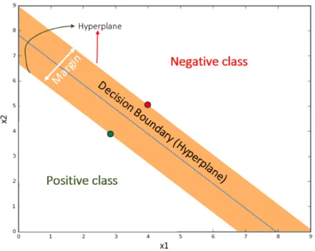
The objective of the SVM classifier is to maximize the decision boundary i.e., maxi-mizing the margin between two classes of training dataset as shown in the figure2.9such that the decision boundary is furthest away from any data point. The separating hyper-plane can be expressed in terms of the data points (red and green from each class in the figure, called support vectors) that are closest to the boundary hyper-planes.

(34)

Figure 2.9: Decision boundary of an SVM classifier with separating hyper-planes on both sides.

(35)

3

Related Work

Coherent and semantically meaningful text generation that mimics the real world text is a crucial task in NLP. Recently, studies have shown that auto-regressive models such as recur-rent neural networks (RNNs) with long short term memory networks (LSTMs) [10,29,31] can achieve excellent performance. However, they suffer from the exposure bias prob-lem [1]. Current techniques proposed to solve this problem, include Gibbs sampling [28], scheduled sampling [1], and adversarial methods, such as SeqGAN [32], LeakGAN [11], MaliGAN [4], RankGAN [17]. Following the framework of generative adversarial net-works (GAN) [9], a discriminator helps the adversarial text generation models to evaluate whether a given text is real or not. Then a generator aims to generate text that is hard to discriminate from the real-world text, which results in a maximized reward signal from dis-criminator via reinforcement learning (RL). The entire text sequence generation of these adversarial techniques can alleviate the problem of exposure bias. Nevertheless, despite their success, these adversarial models still face two challenges such as reward sparsity and mode collapse.

Diverse text generation by employing inverse reinforcement learning (IRL) [27] is proposed to tackle these two challenges. This model assigns instant rewards to the gener-ation policy that generates text sequence by sampling one word at a time, thus allocating

(36)

more dense reward signals. Using an entropy regularized policy gradient [7] as an opti-mization policy results in a more diversified text generator. Dense rewards and an “entropy regularized” policy gradient can alleviate reward sparsity and mode collapse. However, this model requires relatively large number of training samples that are not available for our domain-of-interest.

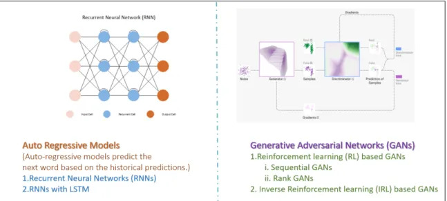
Figure 3.1: State of the art Text generation models

Studying auto-regressive models such as RNN, LSTM (a special kind of RNN), and RL based GANs such as Sequential GANs, Rank GANs, and IRL based GANs provides a better understanding of the disadvantages of current state-of-the-art text generation models.

3.1

Recurrent Neural Networks

Recurrent neural networks (RNNs) [19] are a family of artificial neural networks that are applicable for processing sequential data. The importance of these models that take se-quences as inputs and predict sese-quences as outputs is illustrated by machine translation, language modeling like text generation, named-entity recognition, speech recognition, etc. The typical RNNs that maps sequence to sequence is parameterized by two bias vectors[bh,

(37)

bo], three weight matrices[U, W, V], and a random initial hidden state[h(i)] as shown in

Fig-ure3.2. By using recurrent connections, RNNs remembers a high-dimensional sequence in the form of a hidden state by representing it with a fixed dimensionality. The current pre-dictions [o(t)] made by RNNs are influenced by current hidden state [h(t)] (which represents the history of sequence). So, RNNs combines two sources of inputs, current input [x(t)] (present) and the current hidden state [h(t)] (recent past) to determine the current prediction [o(t)_{], mimicking humans reliance on both past and present information to make decisions.}

Figure 3.2: Recurrent neural network-folded form.

In Figure3.2, the hidden layers of the RNNs have the same weights and bias. So, all hidden layers can be folded in together as a single recurrent layer, called an RNN-folded form.

RNN include the following type of models: Many to Many, One to Many, and Many to One. In this related work, our interest is to study Many to One RNNs (as a generative model) for modeling sequential data. Henceforth, RNNs refer to the Many to One model. The objective of the RNN is to maximize the likelihood of a true token in the training sequence given the previously observed tokens. We used the simplest possible version of

(38)

recurrent neural networks, to help the reader apprehend sequential modeling. The recurrent neural network has an input layerx, a hidden layer h(also called a state or context layer) and output layero as shown in Figure 3.3. The input vector x(t) _{at time} _t _{is a Word2vec}

(W2V) embedding that represents the current word. The output vector (typically of dimen-sions corresponding to the vocabulary size that we are using to train the model) is denoted byo(t), with the hidden layer ash(t) (state of the network). Hidden and output layers are computed as follows: ht =σ U ∗xt+W ∗h(t−1)+bh (3.1) ot=Sof tmax bo+V ∗ht (3.2)

whereσ =Activation function

(39)

3.1.1

Recurrent Neural Networks Training

RNNs training involves two steps, feed-forward propagation (forward pass) and backward propagation through time (BPTT). Unlike feed-forward neural networks (Multi-Layer Per-ceptron), hidden layer values in RNNs are computed using current input and the previous hidden state (sequence history).

Forward Pass

Consider a input sequencex1:T ₌ _x1_{, x}2_{, .., x}t_{, .., x}T _{of length}_T _{given to an RNN. Let} _xt

be the word2vec embedding input at timet, andh(t−1) and h(t) are previous hidden state and current hidden state respectively as shown in the figure3.3.

The hidden state value at timet can be calculated by combining the previous hidden stateh(t−1) _{and current input}_xt _{as shown in equation}_3.1_{. Intuitively, the current hidden}

state represents both present x(t) _{and recent past information} _x1:t−1_{. Usually, the initial}

hidden stateh(i)_{is set to zero. But several research studies showed that RNN performance}

and stability improved by using nonzero initial hidden state values [35].

Current output ot _{can be computed by using the current hidden state} _ht _{as shown in}

equation3.2. Intuitively, current outputot is predicted based on the sequence x(1:t). The output vectorotrepresents the probability distribution of the next token given the previous token x(t) _{in the sequence and context} _x1:t−1 _{(hidden state).} _{Sof tmax} _{assures that this}

probability distribution is valid, i.e., 1 > ot

m > 0 (the probability of each token in the

output vector is greater than zero and less than one) for any token m and Pk m=1o

t m = 1

(the sum of the probabilities of all token in the output vector is equal to 1), wherek is size of the vocabulary.

The objective of the RNN is to maximize the likelihood of a true token in the training sequence given the previously observed tokens. So, we consider cross-entropy to calculate an error vector (loss or cost vector) at every single training step as shown in equation3.3, and weights are updated with the BPTT algorithm. To compute a cost vector we could also

(40)

use negative log-likelihood and maximum likelihood estimation. The relation between the three cost functions: maximize likelihood estimation→minimize negative log-likelihood

→minimize cross-entropy) is as follows.

Jt=−X

k

ytlog ot (3.3)

whereJt =Cross-entropy, ytis the target one-hot encoded vector (which the actual token in the sequence i.e.,x(t+1)).

The targetyt_{is a one-hot encoded vector where position of token}_x(t+1) _{(that follows}

the training sequencex1:t_{) is set to 1. So, the equation}_3.3_{can be rewritten as follows:}

Jt =−X

k

1log ot (3.4)

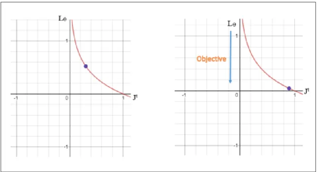
The overall cost is equal to the sum of the errors (according to cross entropy) of the entire sequence of the lengthT. The objective is to minimize the overall cost as shown in Figure

3.4, which maximizes the likelihood of the predicting the true token in the training sequence given the previously observed tokens.

Lθ = 1 T T X t=1 Jt (3.5)

whereLθ =Cost function (optimization or objective function) with parameterθ.

RNN forward pass training with example

Let us look at the RNN forward pass training with the following example tweet: He is

not that retard. The feeding of tokens (he, is, not, that, retard) in the sequence occurs as

(41)

Figure 3.4: The left plot represents Cross entropy vs Cost function. The right plot repre-sents the objective i.e., Minimizing the cost.

The current hidden state h(t) can be calculated by considering current input x(t)= “not”, and the sequence of tokens until timeti.e.,h(t−1).

Current hidden stateh(t) = (xt+h(t−1)) =(not + (He, is))

= (current token+sequence of tokensx1:t−1)

The output vectorotrepresents the probability distribution of the next token given the previous tokenx(t) _{in the sequence and context}_x1:t−1 _{(hidden state). Here, token “is” has}

a high probability but the token “that” is the true token in the sequence.

probability of each tokenot= [0.20,0.30, 0.15,0.22, 0.13] = [He,is, not,that, retard]

(42)

Figure 3.5: Recurrent neural network - training with example

target one-hot encoding vector and output vector as shown in Figure 3.6. Here 0.657 is the error (as shown in the example cost calculation 3.6). The objective of training is to minimize this 0.657 to 0. The cost functionLθtakes the average of the errors calculated at

each step and updates the parameter of the modelθwith the BPTT algorithm.

Figure 3.6: A recurrent neural network with one hot encoded targets

(43)

the completely shaded circle is the true token in sequence. Multiplication of the target one-hot encoded vector and the output vector ensures maximizing the prediction of the true token during generation.

Targetyt= [0,0,0,1,0] =that

Cross entropyJt=H(target one-hot encoded vector, output vector)

=H([0, 0, 0, 1, 0], [0.20, 0.30, 0.15, 0.22, 0.13])

=[0, 0, 0, 1, 0][log(0.20), log(0.30), log(0.15), log(0.22), log(0.13)]

=−(1∗log(0.22)) =−(−0.657) = 0.657

(3.6)

Back Propagation Through Time (BPTT)

During the training of an RNN, an error can be propagated further in time (multiple layers) to remember longer training sequences. Generally, we consider the full sequence (tweet) as one example during training, so total loss is just the average of the errors at each time step.

Recall that our objective is to compute the gradients of the errors concerning the weights U, V, W and then optimize the parameter θ using gradient descent. Just like the losses that we add at each time step, we also add the gradients at each time step for each training sequence during training : _∂W∂J =P

t ∂Jt ∂W

We use the chain rule of differentiation to compute the gradients. We apply the back-propagation algorithm starting from the error at the current token (when timet = T) and propagates this backward all the way (timet = 1) to the initial token. We provideJt_{as an}

(44)

∂Jt ∂V = ∂Jt ∂ot ∂ot ∂V = ∂J t ∂ot ∂ot ∂Zt ∂Zt ∂V = (yt−ot)⊗ht (3.7)

whereZt ₌_{V h}t_{, and}_⊗_{is the outer product between two vectors. From the derivation,}

we can say that computing gradients for V only depends upon ot, yt, ht (simple matrix multiplications between them).

But computing the derivations of W, U ( ∂J_∂Wt ,and ∂J_∂Ut) are different. Following the equation on the chain rule of differentiation for W provides a justification:

∂Jt ∂W = ∂Jt ∂ot ∂ot ∂ht ∂ht ∂W (3.8)

Now, note thatht ₌_{σ U} _∗_xt₊_W _∗_h(t−1)

depends onh(t−1)_{, which again depends}

on W and h(t−2)_{, and so on as shown in the figure} _3.7_{. So during derivation we can not}

consider h(t−1) _{as constant. We must reapply the chain rule, resulting in the following}

equation: ∂Jt ∂W = T X ts=1 ∂Jt ∂ot ∂ot ∂ht ∂ht ∂hts ∂hts ∂W (3.9)

Wheretsis a time step. As the same weightW is used in each time step until the final time step (i.e., from time ts = 1 to ts = t) that we are concerned about, we must back propagate the gradients from timets =tthrough the recurrent network layers all the way tots= 1

BPTT is very similar to standard back-propagation that we apply in deep neural feed-forward networks. The major difference in BPTT is that we add gradients for weight pa-rameter W at each time step. Vanilla neural networks do not share weights papa-rameters (or other parameters) across all the layers, hence we do not need to add these gradients. Similar to standard propagation, BPTT seems to be an elegant name for regular

(45)

back-propagation on an unfolded RNN. We could therefore define a delta vector and propagates backward. Example:δ_(t(t)₋₁₎ = _∂h∂J(t−t1) = ∂Jt ∂ht ∂ht ∂h(t−1) ∂h(t−1)

∂h(t−2). We can apply same equations to

other layers as well.

Figure 3.7: A recurrent neural network - Back Propagation through time

As sequences (tweets) getting longer (20 tokens or more), gradients from the end of the sequence can not reach to the beginning of the sequence. So, BPTT can not update the parameters at the beginning layers and that makes it difficult to train vanilla (standard) RNN. In practice, many people reduce back-propagation to a few layers.

3.1.2

Problems with RNN Training

Long Term Dependencies

The major idea behind RNNs is that they can connect previous and present information to predict the future. Sometimes, RNN fails to connect and utilize historical information to predict future tasks. The success of a standard RNN is determined by the distance between the relevant information and its need in future time step to predict the output.

At times, having recent information is sufficient to predict the present task. For ex-ample, consider a language model that is trying to predict the next token with maximum

(46)

probability given the previous sequence of tokens. If the model is trying to predict the next token in “Airplane is ready to take ...”, then the apparent next token, in this case, is “off”. The model does not require further context. In this kind of scenarios, RNN can learn past information and utilize it effectively because the distance between the relevant information and the place it is required to predict the next token is small.

However, there are also instances where the model needs more context. Consider an example of a long sequence “I grew up in Mexico...I speak Spanish fluently”(as shown in the figure 3.8). In this example, the part “I speak ” predicts that next token probably would be the name of a language, but to predict which language, the model needs the context of Mexico (from the beginning of the sequence). In this example, the distance between the relevant information and the place it is needed is long. Unfortunately, as the sequences grow longer, it is entirely possible that the distance between the relevant information increases, which makes Vanilla RNN language models ineffective for learning longer-term dependencies(connecting relevant information in longer sequences).

(47)

In Figure 3.8, the distance between relevant information “Mexico” and the place it is needed to predict the name of the language “Spanish” is long. Here hi is initial hidden

state,Otis output attthtime step. Also, every hidden state is computed using recent history

and current input.

Theoretically, standard RNNs have the absolute capability of handling sequences with long term dependencies. A researcher should carefully select parameters for the RNN language model to address this problem. In practice, RNNs fail to learn long term depen-dencies. The problem was deeply explored by Bengio, et al., (1994) and Hochreiter (1991), German [13,3]. RNNs are unable to learn long-term dependencies for two reasons: Van-ishing gradients, and exploding gradients.

Vanishing Gradients

Learning longer sequences requires RNN with deep hidden layers. Commonly, including more hidden layers makes the RNN model able to learn complex arbitrary functions to effectively predict future tasks. For example, if we are training an RNN model to learn and generate 32 length sequences, then the RNN model requires 32 hidden layers (each for one token). Applying gradient-based optimization techniques (like BPTT) on these RNNs with deep hidden layers cause the vanishing gradient problem while training.

Loss (error) gradient is the direction and value computed during the training of net-work that is utilized to optimize the netnet-work parameters (weights and biases) in the desired direction (gradient descent decreases parameter values and gradient ascent increases pa-rameter values) by right magnitude. Generally, researches apply gradient descent (∇) in their work. So, in this related work also, gradient descent is applied during optimiza-tion. Now, when we execute Back Propagation Through Time, i.e., passing gradients of error(loss) with respect to weights in the backward direction (from time ts=T to ts=1), the gradients become increasingly while propagating backward in the network as shown in Figure3.11. This slows the learning ability of the neurons in the initial layers of the RNN.

(48)

That makes them hard to train. As the initial layers of the deep RNN are very important to identify the core elements of the input sequence, this limitation can lead to inaccurate sequences. This also causes learning inability to remember and retrieve long-term depen-dencies at a later point in time to predict the next token.

Let us take a closer look at the gradient derivation3.9 in the BPTT section to under-stand what causes these gradients to become smaller and smaller as they propagate to initial layers. ∂Jt ∂W = T X ts=1 ∂Jt ∂ot ∂ot ∂ht ∂ht ∂hts ∂hts ∂W

Here _∂h∂htst is a chain rule in itself! For example,

∂ht ∂h(t−2) = ∂ht ∂h(t−1) ∂h(t−1) ∂h(t−2). Taking

the derivative of the vector function with respect to a vector results in a Jacobian matrix (containing a first-order partial derivative for a vector function). We can represent the above gradient as follows: ∂Jt ∂W = T X ts=1 ∂Jt ∂ot ∂ot ∂ht T Y t=ts+1 ∂ht ∂h(t−1) ! ∂hts ∂W (3.10)

According to Pascanu, et al., (2013) [23], the upper bound of the L2-norm (think of it as absolute value) of the above Jacobian matrix is 1. This is because the sigmoid and tanh activation functions map all values into a range in between 1 to -1. The derivation of the sigmoid and tanh bounded by 0.25 and 1 respectively are shown in Figure3.9,3.10.

As in Figures3.9,3.10, the derivatives of sigmoid andtanhbecome flat and approach zero at both ends. When the derivatives approach these flat ends, the related neurons reach a saturated state. These zero gradients make the other gradients in the previous layers approach zero. This is caused by multiple matrix multiplications with the Jacobian matrix with small values (which are close to zero). Thus, the gradient values shrink exponentially fast and eventually vanish after certain time steps as shown in the figure 3.11. So, the

(49)

Figure 3.9: Sigmoid f(x) and it’s derivative ∂f_∂x

gradient contribution from distant layers does not reach the layers at the beginning. This makes RNN model fail to learn the relation between the “Mexico” and “Spanish” because the gradients (error) from “Spanish” can not reach (does not show impact) to “Mexico” (the beginning layer). Model end up not learning long-term dependencies. This Vanishing gradient problem is not exclusive to RNN. Even vanilla neural networks that use stochastic gradient descent for optimization have the same problem. It is just that RNNs tend to have deeper hidden layers (generally according to the size of the sequence). We expect this problem more often.

In figure3.11, the size of the∇(gradient descent) indicates the gradient value.

Exploding Gradients

Depending on the activation functions and network parameters that are applied to RNNs, the model could end up with Jacobian matrices with large values that cause exploding gra-dients instead of vanishing gragra-dients. Hence this is called the exploding gradient problem.

(50)

Figure 3.10: Tanh f(x) and it’s derivative ∂f_∂x

Vanishing gradients have received more attention than exploding gradients for two reasons. First, identification of exploding gradients is easy because gradients will become Not-A-Number(NAN) as shown in Figure 3.12 and crash the model. Second, there is a simple clipping solution available i.e., by carefully pre-defining the threshold values to clip the gradients, one can reduce the exploding gradient problem as shown in Figure 3.13. Van-ishing gradients are harder to solve because it is not evident when they happen or how to handle them.

In figure3.12, the size of the∇(gradient descent) indicates the gradient value. Error gradients can add up during optimization and cause very large gradients. Consecutively, this results in large updates to model parameters and causes an unstable neural network. In the worst case, the magnitude of the parameters can become so large as to overflow and cause in Not-A-Number (NAN) value. Here, gradient contribution from distant layers did not reach the layers at the beginning. This makes RNN model fail to learn the relation between the Mexico and Spanish because the gradients (error) from Spanish can not reach

(51)

Figure 3.11: Recurrent Neural network - Vanishing Gradient problem

(does not show impact) to Mexico (the beginning layer). The model cannot learning long-term dependencies.

The left side of the figure3.13is gradient without clipping and the gradients explode. The right side figure 3.13is gradient clipping that confines the gradient values within the threshold limits. Here,J(w, b)model based on the weight w and biases b.

Solution to Vanishing and Exploding gradient problems

As we discussed earlier, the vanishing gradient problem is hard to solve compared to ex-ploding gradient problem. However, there are a few ways to counter the vanishing gradient problem. Careful initialization of weight matrices (particularly matrix W) and regulariza-tion can lower the effects the vanishing gradients. Generally, researches prefer the Rectified Linear Unit (ReLU) activation function as an alternative to sigmoid or tanh to combat the

(52)

Figure 3.12: Recurrent Neural network - Exploding Gradient problem

vanishing gradient problem. This is because the ReLU derivative is a either 0 or 1 as shown in Figure3.14. So, it is not as expected to suffer from the vanishing gradient problem. A more preferred solution to use is to use Long-short Term Memory (LSTM) or Gated Re-current Units (GRU) units in an RNN architecture. Most widely used LSTMs models in Natural Language Processing (NLP) community were proposed in 1997 [14]. GRUs, ini-tially proposed in 2014 [5], are a simplified variant of LSTMs. Both of these (LSTMs, and GRUs - special kind of RNN) architectures were especially created to handle these van-ishing and exploding gradient problems and effectively learn the long-term dependencies. Researchers tailor different variations of LSTMs according to the problem they are solving. So, we will discuss LSTMs in detail in the next section.

(53)

Figure 3.13: Gradient clipping

3.2

Long Short Term Memory (LSTM)

LSTMs are especially created to effectively solve long-range dependencies. Memorizing information about longer sequences and utilizing this information in a later point of time is their default behavior (and LSTMs do not struggle to learn long term dependencies). Stan-dard Vanilla RNNs have the form of a chain of redundant modules of a neural network(with simple activation layers like single Tanh) as shown in the figure3.15. LSTMs also have a similar chain-like structure as in the standard vanilla RNNs, but interestingly the redundant modules have four neural network layers interact in a special way as shown in Figure3.16. In Figure3.16,ft_{is a forget gate ( a neural network with sigmoid),}_it_{is an input gate}

(a neural network with Sigmoid),Cˆt _{is a temporary cell state or candidate layer (a neural}

network with Tanh), opt _{output gate (a neural network with sigmoid),} _ht _{hidden stat (a}

vector),ctcurrent memory or cell state (a vector).

In Figure3.17, each line in the LSTM architecture carries an entire vector from one node to another node. Point-wise operations like vector multiplication and addition are

(54)

rep-Figure 3.14: ReLU activation functionf(x)and it’s derivative ∂f_∂x

resented by pink circles. Neural networks layers are represented by yellow rectangles. Con-catenation denoted by merging lines, and forking lines indicate information being copied and passed to a different location.

The memory (cell) state (horizontal line passing at the top of architecture as shown in Figure3.18) plays a main role in LSTM. This cell value runs over the chain of redundant modules of LSTM architecture carrying memory. In this way, the memory value has only a few linear interactions. It is very easy for the model to pass a memory value unchanged.

The LSTMs can update (by adding new information or discarding current informa-tion) a memory value carrying by cell state with the help of carefully regulated structures called gates. Gates can control the information that goes to the cell state. These input (it_{), forget (}_ft_{), and output gates (}_opt_{) are built out of sigmoid networks and a point-wise}

multiplication operation.

The sigmoid activation function maps the inputs to the range between 0 and 1. In-tuitively, sigmoid describes the amount of information from each component it should let

(55)

Figure 3.15: Standard Vanilla RNNs.

Figure 3.16: LSTM

through. Zero means it will not allow any information to the cell state and whereas one means it will allow all information. So, sigmoid activation functions at all three gates decide the amount (between 1 and 0) of information they will allow to the cell state.

LSTM Working Mechanism with example

In figure3.19, LSTM remembers long term dependency between “Mexico” and “Span-ish” with the help of cell state.

(56)

Figure 3.17: Notations used in the LSTM.

Figure 3.18: LSTM - Memory (cell) value propagation

In Table3.1, the cell state remembers a country name by setting its memory as 1 and carries this information to a later point in time (“speak”) to predict the name of the language (“Spanish”). After the utilization of this information, the cell state discards this memory and sets its memory to 0.

Forget Gate

Initially, the model must decide what information it should discard from the memory that is carrying by cell state. A forget layer (sigmoid activation function) takes this decision. According to current input at time stept(xt) and previous hidden state (h(t−1)), forget gates output a number between 1 and 0 as shown in the figure 3.20. Point-wise multiplication between the previous cell statec(t−1) _{and resultant sigmoid values (between 0 and 1) from}

Memory value 0 0 0 0 1 1 1 1 0 0

Input token I grew up in Mexico ... I speak Spanish fluently Table 3.1: Passing of memory value through the chain of repeated layers.

(57)

Figure 3.19: Working Mechanism of LSTM with example.

the forget gate decides how much information the model will throw away.

ft =σ U ∗xt+W ∗h(t−1) (3.11)

Let us look into the example as shown in the figure3.20. In this example, the cell state remembers that “Mexico” predicts “Spanish”. Suppose, if the model detects a new country “French” in the training sequence, then the model must forget the old information about the country to predict the new language “French”. So, the forget gate discards memory about the name of the country after it is utilized in the model to detect the name of the language.

Input Gate&Candidate layer

After the forget gate step, the model must decide what new information it is going to add to the memory carrying by cell state. This process consists of two parts. The first part is the input gate (it_{) layer that helps the model decide which values it will update. The second}

(58)

Figure 3.20: LSTM - Forget fate (ft)

these two parts to update the memory cell.

ˆ

ct₌_{tanh U} _∗_xt₊_W _∗_h(t−1)

(3.12)

it=σ U∗xt+W ∗h(t−1) (3.13)

Figure 3.21: LSTM - input gate (it₎

(59)

into new memory value ct_{. The resultant vector of new candidate values from point-wise}

multiplication betweenit_and_Cˆt_{decides the scale at which the memory values will update.}

The model just needed to do a point-wise linear operation between c(t−1) _{and resultant}

vector of new candidate values to make this update happen as shown in Figure3.22.

ct=ft∗ct−1+it∗Cˆt _(3.14)

Figure 3.22: LSTM - updating its cell state

As we have seen in the above example, this is where the model will actually update its memory value when it looks at the name of the country “Mexico” as input.

Output Gate

Ultimately, the model must decide what it is going to output ot_{. The output is just a}

filtered version of memory value carrying by cell state. In this step, initially the model executes a sigmoid layer that will decide what parts of cell state it will output. Then the model will execute point-wise multiplication between the cell state that passed through the tanh layer (to change the range of values between -1 to 1) and output from the sigmoid layer. This multiplication gives the current hidden state (ht_{) which contains only those}

(60)

opt=σ U ∗xt+W ∗h(t−1) (3.15)

ht =o