DOI 10.1007/s10479-015-2086-z
Designing multi-period supply chain network considering
risk and emission: a multi-objective approach
Ravi Shankar Kumar1 · Alok Choudhary2 · Soudagar A. K. Irfan Babu3 · Sri Krishna Kumar3 ·A. Goswami1 ·M. K. Tiwari3
© The Author(s) 2016. This article is published with open access at Springerlink.com
Abstract This research formulates a multi-objective problem (MOP) for supply chain net-work (SCN) design by incorporating the issues of social relationship, carbon emissions, and supply chain risks such as disruption and opportunism. The proposed MOP includes three conflicting objectives: maximization of total profit, minimization of supply disruption and opportunism risks, and minimization of carbon emission considering a number of supply chain constraints. Furthermore, this research analyses the effect of social relationship lev-els between different tiers of SCN on the profitability, risk, and emission over the time. In this regard, we focus on responding to the following questions. (1) How does the evolving social relationship affect the objectives of the supply chain (SC)? (2) How do the upstream firms’ relationships affect the relationships of downstream firms, and how these relationships influence the objectives of the SC? (3) How does the supply disruption risk interact with the opportunism risk through supply chain relationships, and how these risks affect the objectives of the SC? (4) How do these three conflicting objectives trade-off? A Pareto-based multi-objective evolutionary algorithm–non-dominated sorting genetic algorithm-II (NSGA-II) has been employed to solve the presented problem. In order to improve the quality of solutions, tuning parameters of the NSGA-II are modulated using Taguchi approach. An illustrative example is presented to manifest the capability of the model and the algorithm. The results obtained evince the robust performance of the proposed MOP.
Keywords Supply chain network·Social relationship·Risk management·Emission·
Multi-objective optimization·Pareto optimal
B
Alok Choudhary [email protected]1 Department of Mathematics, Indian Institute of Technology, Kharagpur 721302, India 2 School of Business and Economics, Loughborough University, Leicestershire LE113TU, UK 3 Department of Industrial and Systems Engineering, Indian Institute of Technology,
1 Introduction
Owing to tremendous development in technology, globalization of markets, and heightened customers’ expectations, today’s market competition has shifted from competitive inde-pendent firms to competitive SCs. E-business is another prominent factor that encourages
different firms to compete as an integral part of SCs (Zhang 2006).Rice and Hoppe(2001)
and Xiao and Yang (2008) highlighted that now the competition is SC versus SC instead of
traditional company versus company. There are several instances of SC versus SC competi-tion in different industries such as Microsoft-HTC and Nokia-Symbian SCs in the electronic
industries (Xiao and Yang2008), Amazon.com and barnesandonoble.com in the book
mar-ket (Bernstein and Federgruen 2004), Dell’s competition against Apple in personal computer
market (Rice and Hoppe 2001) etc.
Supply chain network (SCN) is a strategic level decision making problem that deals with various issues such as determination of size, number and location of facilities in a supply chain, tactical decision making such as distribution, transportation and inventory manage-ment policies, and also involves operational decisions such as fulfilmanage-ment of customer demand,
pricing and customer service level (Farahani et al. 2014). In today’s global competitive era,
companies strive to minimize the relevant costs and maximize their opportunities in the market, and thereby they consistently focus on the improving partnerships and alliance
rela-tionships. According toCroom et al.(2000), any endeavour in managing the information
and/or material flow is likely to be ineffective in absent of effective supply chain organi-zational relationship. Moreover, there is an increasing concern over environmental, health and safety regulations issues of workers involved in the production processes. For example, leading corporations like Apple, Liz Claiborne, Disney, Nike and Wal-Mart have faced dam-aging media reports, external pressure from activists, and internal pressure from investors demanding that companies acknowledge responsibility for labour rights’ abuses in factories (Cruz and Wakolbinger 2008, and references therein). Consequently, companies show their interest in tackling of social and environmental issues.
Motivated by these factors, we model a multi-objective multi-period (MOMP) integrated supply chain model that considers the effects of social relationship levels in presence of disruption risk and opportunism risk in a multi-tier SCN. The environmental issue is also incorporated in developing the proposed mathematical model of SCN. In this manner, this research primarily focuses on responding the following questions:
(1) What are the effects of the evolving social relationships on price and demands, and finally on the objectives (profitability, risk and emission) of supply chain?
(2) How do the upstream firms’ relationships affect the relationships of downstream firms, and how these relationships influence the objectives of the SC?
(3) How does the supply disruption risk interact with the opportunism risk through supply chain relationships, and how these risks affect the objectives of the SC?
(4) How do three conflicting objectives interact and trade-off with each other?
This research formulates a multi-objective problem (MOP) for supply chain network (SCN) design by incorporating the issues of social relationship, carbon emissions, and supply chain risks such as disruption and opportunism. The proposed MOP includes three conflicting objectives: maximization of total profit, minimization of supply disruption and opportunism risks, and minimization of carbon emission considering a number of supply chain constraints. Furthermore, this research analyses the effect of social relationship levels between different tiers of SCN on the profitability, risk, and emission over the time.
NSGA-II is an efficient algorithm to solve a MOP particularly when the number of
objec-tives is more (Deb et al. 2002). It is a population based random search algorithm, in which
solution quality is improved over iterations. The proposed MOMP integrated SCN has three conflicting objectives and therefore in order to obtain good near optimal solution, we employ NSGA-II to our mathematical model. Moreover, one of the main motivations to choose this approach is its successful and proven application in various other domains of multi-objective optimization (MOO). In order to find the better solution, this research chooses the algorith-mic parameters of NSGA-II by using Taguchi method. It is well known that Taguchi method is based upon statistical experimental design that evaluate and implement improvement in
products, process and equipment (Tiwari et al. 2010).
The rest of the paper is organized as follows: Sect.2 provides brief literature review.
Section3discusses the mathematical model followed by description of solution
methodolo-gies: MOEA and NSGA-II in Sect.4. Section5presents computational studies. Section6
discusses tuning of parameters of NSGA-II using Taguchi method. Results of numerical
experiment and discussion are presented in Sect.6followed by conclusion and direction for
future research in Sect.8.
2 Literature review
This section reviews the relevant literature in specific domains of modelling of supply chain relationships, modelling of supply chain risks including opportunism and disruption and models which included carbon emission as an objective in supply chains. In addition, we also reviewed several multi-objective models used to solve these problems to make a case for the application of NSGA II.
Supply chain relationship issues in SCs have received a great research attention in the
area of operations management, economics and marketing (Cruz and Liu 2011). A
competi-tive advantage and efficiencies flexibility could be achieved by promoting the collaboracompeti-tive relationships amongst supply chain partners. Moreover, long-term collaborative relationship may result in creating unique value, which could only be possible when the partners make cooperative efforts rather than independent. Its an on-going process to lower acquisition and
operating costs (Nyaga et al. 2010).Daugherty et al.(2006), suggested that the firms build
multiple collaborative relationship to accomplish higher service level, increased flexibility, increased customers’ satisfaction, reduced cycle times and lower risks. Moreover, strong multiple relationships encourage firms to change the marketplaces and to create customer
value and loyalty, finally leading to maximum profit margin (Cruz and Liu 2011). Dyer
(2000) found that the collaborative behaviours of supply chain tend to be more accountable
to reduce the supply chain-wide costs (costs associated with negotiating, monitoring, and
enforcing contracts). According toUzzi(1997) andGadde and Snehota(2000), the negative
effects related to dependency of supply chain partners can be mitigated through the strong
multiple relationships.Krause et al.(2007) recognized that commitment and social capital
accumulation among the stakeholders are important complementary conditions that estab-lish performance goals and improve buying performance. However, most of these research focussed on establishing the benefits of having multiple relationships. Very negligible work has been done o demonstrate the effects of the evolving social relationships on price and demands. In addition, tvery limited work investigated the impact of these relationships on firms’ objectives such as profitability, risk mitigation and carbon emission in a supply chain.
Supply chain risks including disruption and its management have received a great atten-tion in academic literature as well as in industrial applicaatten-tions. Supply chain disrupatten-tion is an
unanticipated event that spawns disturbance in normal flow of material within SCN (
Craig-head et al. 2007). Supply chain risk management (SCRM) has emerged due to various reasons including globalization, volatile market places, crisis and calamities etc., and substantially
more susceptible than traditional integrated production planning (Hoffmann et al. 2013). An
empirical study of around 800 instances of supply chain disruptions conducted by Hendricks
and Singhal (2005) suggested that the companies that suffered with supply chain disruptions
earned lower share prices return (33–40 % lesser) and higher share price volatility (13.5 % higher) compared to the general market benchmarks. In light of three dimensions of supply
disruption risk namely magnitude, probability, and overall supply disruption risk,Ellis et al.
(2010) empirically explored that both the probability and magnitude are important to overall
perception of supply disruption risk. According toCruz and Liu(2011), supply chain
dis-ruptions have worldwide impacts and therefore in order to capture the complex interactions among stakeholders, a holistic and system-wide SCN modelling and analysis is essential. Nonetheless, very limited researchers have examined SCRM considering supply chain rela-tionship issues. An exhaustive latest review related to supply chain disruption is presented in
Ellis et al.(2010).
In addition to supply disruption risk, opportunism risk is also studied in several SCN
liter-atures (e.g.,Tangpong et al. 2010;Vandenbosch and Stephen 2010). Opportunism is lack of
candour/honesty in transaction and self-interest seeking with guile, which also includes fal-sification of expense reports, breach of distribution contracts, bait-and-switch tactics, quality
shirking, and violation of promotion agreements (Cruz and Liu 2011;Handley and Benton
2012). Very little or negligible work has been done to combine social relationship, supply
dis-ruption and opportunism risks in designing SCN and therefore an identified research gaps to pursue the proposed research. In addition, environmental concerns have also been considered in this research.
Increasing awareness of the need of environmental protection and sustainability stimulate government, consumers, local communities, and stakeholders groups to exert pressure on companies to effectively incorporate sustainability issues into their supply chain
manage-ment practices (Cruz 2013;Gold et al. 2010). Now a day, environmental performance at any
stage of supply chain is one of the most crucial criteria to evaluate the reputation of a com-pany. As an example of public awareness campaigns by advocacy group, many companies such as McDonalds, Mitsubishi, Monsanto, Nestle, Shell, and Texaco have suffered with
damages of reputation and sales (Svendsen et al. 2001). In recent years, increasing
environ-mental concerns enforced researchers to deal with environenviron-mental risks. The increased focus on environment highly influences the supply chain schemes. Consequently, stakeholders of an organization are forced to stretch their responsibility for their product beyond their sales
and delivery locations (Bloemhof-Ruwaard et al. 1995). An exhaustive review concentrating
about environmental issues is available inCruz and Wakolbinger(2008),Cruz(2013) and
Tseng and Hung (2014). However, social relationship is capable to lead the programs of col-laborative waste reduction, cost-effective environmental solutions, environmental innovation at the interface, the rapid development and uptake of innovation in environmental technolo-gies, and allows firms to better understand the environmental impact of their supply chains (Simpson and Power 2005).
Environmental issue in sustainable SC and closed-loop SC has been modelled by many
researchers such asWang and Gunasekaran(2015), De Giovanni (2014),Costa et al.(2014).
Zakeri (2014) discussed the impact of carbon trading schemes and its impact on tactical supply
model to manage supply chains under two carbon regulatory schemes. They implemented
their model using real data from an Australian furniture manufacturing company.Fahimnia
et al.(2013) developed a SC model in which environmental issue is tackled by minimization
of emission.Battini et al.(2014) proposed a sustainable SC focusing on CO2emission due
to transportation, in which an economic order quantity is derived for material purchasing.
Zakeri et al.(2015) discussed the impact of carbon trading schemes and its impact on tactical
supply chain planning decision.Rezaee et al. (2015) extendedFahimnia et al.(2015a,b)
model by considering stochastic demand.Andriolo et al.(2015) proposed a bi-objective SC
focusing on minimization of total cost including transportation, while second objective is to minimize the carbon emission. An exhaustive review of modelling of environmental issues
in supply chain is conductedFahimnia et al.(2015a,b).
The aforementioned discussion indicates that negligible research has been done in devel-oping models which have simultaneously dealt with social relationship, supply disruption and opportunism risks, and emissions. Furthermore, most of the previous models have focussed on single-objective optimization process. However, real-life supply chain environment is very sophisticated and complex in nature, and involves optimization of several incommensurable objectives simultaneously. Therefore, there is need to consider the multi-objective nature of SCN problems. Researchers have shown a great interest in recent years to use multi-objective
optimization techniques in supply chain modelling problems such asLiao et al.(2011), Soysal
et al. (2014), Zhang et al. (2013),Govindan et al.(2014), Liang et al. (2013) and Devika et al.
(2014) in various domains of supply chain. However, none of this research simultaneously
considered social-relationship, risk, and emission in supply chain.
In recent years, researchers have shown their interest to use MOO techniques in SC modelling problems. The classical method of solving a MOP is to use weighted sum method that combines all the objective functions into one-objective function and treat it as a single
objective with multiple constraints. Value fraction,ε-constraint, and weighted-matrix are
some other classical methods to solve the MOPs. All these algorithms convert the MOP into single-objective problem (SOP). Other way to solve the MOP is to develop a Pareto-front for
given objectives, and then select the Pareto-front using several methods.Liao et al.(2011)
formulate an MOP for vendor managed inventory (VMI) setup, which integrates the effects of distribution, facility location, and inventory issues, then used a multi-objective evolutionary
algorithm based on the non-dominated sorting genetic algorithm-II (NSGA-II) (seeDeb
et al. 2002) to solve the MOP. Similarly,Govindan et al.(2014) formulated a mathematical model of an MOP to solve environmental issues of food supply chain for perishable product. Furthermore, they employed multi-objective evolutionary algorithm NSGA-II to solve the problem.
Motivated by identified research gaps in literature and the complexity of real-life supply chain environment, we formulate a MOP for multi-tier, multi-period supply chain that simul-taneously includes social relationship, supply disruption and opportunism risks, and emission.
In this research, we present a model [an extension ofCruz and Liu(2011)] to integrate the
concepts of social relationship, supply chain disruption and opportunism risks, and emis-sions. To obtain good near optimal solution, we employ famous and efficient multi-objective based meta-heuristic NSGA-II. One of the main motivations to choose this approach is its successful applicability in various other domains of multi-objective optimization. In addition, it is well known that Taguchi method is based upon statistical experimental design that
eval-uate and implement improvement in products, process and equipment (Tiwari et al. 2010).
This research integrates Taguchi method to tune the algorithmic parameters of NSGA II to improve the quality of solutions obtained by NSGA-II.
3 The MOMP integrated SCN model
This section develops the proposed MOMP integrated SCN model by incorporating the emis-sion and disruption risk. This model is based on the assumption that a centralized deciemis-sion maker makes all decisions of the SCN including the size of shipments between the stake-holders, levels of social relationship, production quantities and inventories in each period. At this stage, our first objective is to maximize the profit of entire supply chain consisting
of the profits of I suppliers, J manufacturers, and K retailers. The second objective is to
minimize the risks including supply disruption and opportunism, while, third objective is to minimize the emission of entire supply chain. Furthermore, we assume that the planning
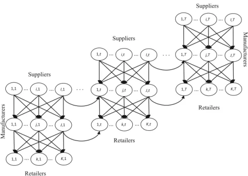
horizon is finite and is discretized intoT periods, as shown in Fig.1. As we endeavour to
extend the model proposed byCruz and Liu(2011), the indices and decision variables used
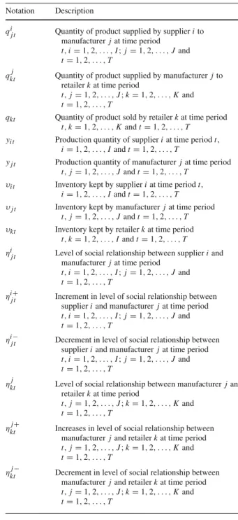
throughout the paper are adopted fromCruz and Liu(2011), and are described in Tables1
and2.
The SCN under consideration comprises of three tiers. The top tiers (i.e. suppliers) provides parts/raw-materials to the manufacturers, who convert them to finished goods, which are then sold to the retailers i.e. the bottom tier of the SCN. The retailers sell these products to the consumers. In our model, we have assumed that there are no constraints on the interaction between the tiers i.e. each manufacturer can procure materials from any of the suppliers, and each of the retailers can acquire products from any of the manufacturers. This would result in
two variables (1) transaction quantity(q)and (2) social relationship level (η) associated with
any pair of supplier and manufacturer, manufacturer and retailer. We have also considered a fixed planning horizon with discretised time periods. The evolution of the SCN over the
planning horizon is shown in Fig.1.
. . . 1,1 1,1 1,1 I,1 i,1 ... ... ... ... ... J,1 K,1 k,1 j,1 ... 1,t 1,t 1,t I,t i,t ... ... ... ... ... J,t K,t k,t j,t ... 1,T 1,T 1,T I,T i,T ... ... ... ... ... J,T K,T k,T j,T ... . . . Suppliers Suppliers Suppliers Retailers Retailers Retailers Manufacturers Manufacturers
Table 1 Indices used throughout
the paper i=1, . . . ,I Supplier
j=1, . . . ,J Manufacturer
k=1, . . . ,K Retailer
t=1, . . . ,T Time period
The model consists ofI number of suppliers,J number of manufacturers,K number of
retailers, and a fixed planning horizonT which is discretized into periods: 1,…,t,…,T. A
typical supplier in the top tier is denoted byi, a typical manufacturer in the middle tier is
denoted by j, and a typical retailer in the bottom tier is denoted byk. As shown in Fig.1,
the nodes (i,t)denotes supplieriin time periodt, node (j,t) represents the manufacturer j
in time periodt, and the node (k,t)denotes the retailerkin time periodt. In summary, the
suppliers (1,…,i,…,I), manufacturers (1,…,j,…,J), and retailers (1,…,k,…K) remain the
same throughout the planning horizon, but the transaction quantities, and social relationship
levels varies with time period. Therefore, the SCN at a time periodtrepresents the level of
transaction quantity and social relationship between the entities of the SC. The indices and
decision variables used throughout the paper are adopted fromCruz and Liu(2011), and are
described in Tables1and2.
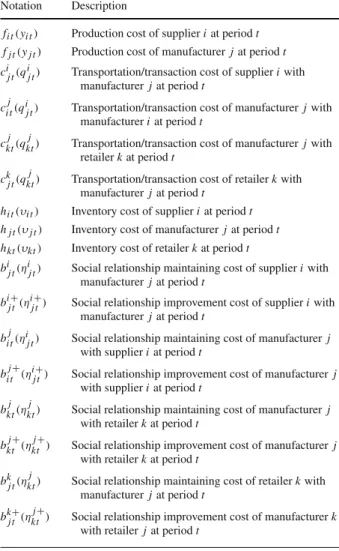
The cost incurred on suppliers, manufacturers, and retailers are described in terms of
transaction and social relationship level in Table3. The production cost for each supplier or
manufacturer at each time periodt is a function of product out-turns. The transaction cost
between stakeholders depends upon product quantity transacted between them. Suppliers, manufacturers and retailers may keep inventory to avoid supply disruption and to quickly deliver product. Thus, inventory cost depends upon quantities of product held for the peri-ods. Furthermore, to mitigate risks associated with SCN, certain level of relationships to be achieved between the supplier and the manufacturer, the manufacturer and the retailer, and vice-versa. To achieve this objective, each stakeholder may spend money in the form of time, service, information sharing, assets or additional personnel. The relationship cost functions reflect the expenditure in order to maintain and/or improve the relationship level. However, relationship establishment and maintenance cost functions for each combination such as supplier–manufacturer or manufacturer–retailer may be distinct. The buyer–seller
interac-tion and communicainterac-tion magnitude changes the relainterac-tionship strength (Crosby and Stephens
1987), and vice-versa. The functional form of social relationship cost may be influenced
by many factors such as the willingness of decision-maker to establish/maintain a level of
social relationship and improvement in level of relationship (Cruz and Liu 2011). The level
of relationship is a real number that lies between zero and one where zero indicates no social relationship and one indicates the strongest possible level of social relationship. The levels of social relationship and the material flows are endogenous and are determined by the decision maker.
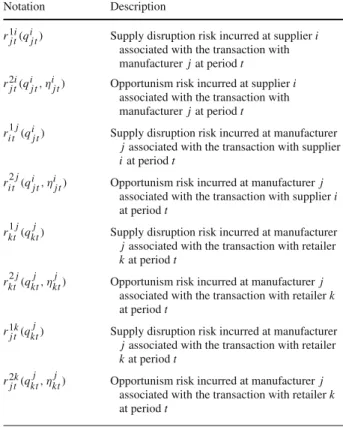
Table4presents the description of the risk functions, which are often inherent in the supply
chain. The risk functions considered in this model are functions of the transaction quantity
and the relationship level.Juttner et al.(2003) highlighted that there are mainly three sources
of supply chain-relevant risk: (1) environmental, e.g., fire, flood, or social-political actions, (2) organizational, e.g., supply disruption, production uncertainties or exchange rate risk,
and (3) network-related risk. Furthermore,Johnson(2001) andNorrman and Jansson(2004)
discussed that lack of cooperation and interaction between the stakeholders within the SC engender network-related risk. This model assumes that each stakeholder faces environmental
Table 2 Description of decision
variables Notation Description
qij t Quantity of product supplied by supplierito manufacturerjat time period
t,i=1,2, . . . ,I;j=1,2, . . . ,Jand
t=1,2, . . . ,T
qktj Quantity of product supplied by manufacturerjto retailerkat time period
t,j=1,2, . . . ,J;k=1,2, . . . ,Kand
t=1,2, . . . ,T
qkt Quantity of product sold by retailerkat time period t,k=1,2, . . . ,Kandt=1,2, . . . ,T
yi t Production quantity of supplieriat time periodt, i=1,2, . . . ,Iandt=1,2, . . . ,T
yj t Production quantity of manufacturerjat time period t,j=1,2, . . . ,Jandt=1,2, . . . ,T
υi t Inventory kept by supplieriat time periodt, i=1,2, . . . ,Iandt=1,2, . . . ,T
υj t Inventory kept by manufacturerjat time period t,j=1,2, . . . ,Jandt=1,2, . . . ,T υkt Inventory kept by retailerkat time period
t,k=1,2, . . . ,Iandt=1,2, . . . ,T ηi
j t Level of social relationship between supplieriand
manufacturerjat time period
t,i=1,2, . . . ,I;j=1,2, . . . ,Jand
t=1,2, . . . ,T ηi+
j t Increment in level of social relationship between
supplieriand manufacturerjat time period
t,i=1,2, . . . ,I;j=1,2, . . . ,Jand
t=1,2, . . . ,T ηi−
j t Decrement in level of social relationship between
supplieriand manufacturerjat time period
t,i=1,2, . . . ,I;j=1,2, . . . ,Jand
t=1,2, . . . ,T ηj
kt Level of social relationship between manufacturerjand
retailerkat time period
t,j=1,2, . . . ,J;k=1,2, . . . ,Kand
t=1,2, . . . ,T ηj+
kt Increases in level of social relationship between
manufacturerjand retailerkat time period
t,j=1,2, . . . ,J;k=1,2, . . . ,Kand
t=1,2, . . . ,T ηj−
kt Decrement in level of social relationship between
manufacturerjand retailerkat time period
t,j=1,2, . . . ,J;k=1,2, . . . ,Kand
t=1,2, . . . ,T
and/or organizational engendered supply disruption risks, and opportunism risk engendered by insufficient cooperation and commitment between the partners of the SCN. In this research, our presented model considers organizational risk, environmental risk and network related risk of supply chain by defining risk as a function of transaction volume and level of social relationship.
Table 3 Description of cost
functions Notation Description
fi t(yi t) Production cost of supplieriat periodt fj t(yj t) Production cost of manufacturerjat periodt cij t(qij t) Transportation/transaction cost of supplieriwith
manufacturerjat periodt
ci tj(qij t) Transportation/transaction cost of manufacturerjwith manufactureriat periodt
cktj(qktj) Transportation/transaction cost of manufacturerjwith retailerkat periodt
ckj t(qktj) Transportation/transaction cost of retailerkwith manufacturerjat periodt
hi t(υi t) Inventory cost of supplieriat periodt hj t(υj t) Inventory cost of manufacturerjat periodt hkt(υkt) Inventory cost of retailerkat periodt
bij t(ηij t) Social relationship maintaining cost of supplieriwith manufacturerjat periodt
bij t+(ηij t+) Social relationship improvement cost of supplieriwith manufacturerjat periodt
bi tj(ηij t) Social relationship maintaining cost of manufacturerj
with supplieriat periodt
bi tj+(ηij t+) Social relationship improvement cost of manufacturerj
with supplieriat periodt
bktj(ηktj) Social relationship maintaining cost of manufacturerj
with retailerkat periodt
bktj+(ηktj+) Social relationship improvement cost of manufacturerj
with retailerkat periodt
bkj t(ηktj) Social relationship maintaining cost of retailerkwith manufacturerjat periodt
bkj t+(ηktj+) Social relationship improvement cost of manufacturerk
with retailerjat periodt
Table 5presents a description of the emission functions. The growing environmental
concerns motivate to incorporate the environmental issues specifically carbon emission while modelling a SC problem (Qiu et al. 2001). The amount of emissions generated depends upon the volume of product produced and transacted as well as level of social relationship in
current and previous periods (Cruz and Wakolbinger 2008). In this model, we assume that the
decision maker seeks to minimize the total emissions generated by suppliers, manufacturers and retailers in the process of production as well as in the process of product delivery to the next tier of supply chain.
The inverse demand function associated with the retail market is presented in Table6.
3.1 Profit maximization
The first objective of this MOP is to maximize the total profit of entire supply chain over
the planning horizonT. Most of the decision variables considered in this model are adopted
Table 4 Description of risk
functions Notation Description
r1j ti(qij t) Supply disruption risk incurred at supplieri
associated with the transaction with manufacturerjat periodt
r2j ti(qij t, ηij t) Opportunism risk incurred at supplieri
associated with the transaction with manufacturerjat periodt
ri t1j(qij t) Supply disruption risk incurred at manufacturer
jassociated with the transaction with supplier
iat periodt
ri t2j(qij t, ηij t) Opportunism risk incurred at manufacturerj
associated with the transaction with supplieri
at periodt
rkt1j(qktj) Supply disruption risk incurred at manufacturer
jassociated with the transaction with retailer
kat periodt
rkt2j(qktj, ηktj) Opportunism risk incurred at manufacturerj
associated with the transaction with retailerk
at periodt
r1j tk(qktj) Supply disruption risk incurred at manufacturer
jassociated with the transaction with retailer
kat periodt
r2j tk(qktj, ηktj) Opportunism risk incurred at manufacturerj
associated with the transaction with retailerk
at periodt
Table 5 Description of emission
functions Notation Description
eij t(qij t, ηij t) Emission at supplieriassociated with manufacturer
jat periodt
ei tj(qij t, ηij t) Emission at manufacturerjassociated with supplier
iat periodt
ektj(qktj, ηktj) Emission at manufacturerjassociated with retailer
kat periodt
ekj t(qktj, ηktj) Emission at retailerkassociated with manufacturer
jat periodt
Table 6 Inverse demand
function Notation Description
ρ3kt(dt) Inverse demand function in the retail market
described in Table3. The profit of entire supply chain is the sum of the profits earned by the
suppliers, manufacturers, and retailers over the periodsT. Hence, the profit maximization
max T t=1 I i=1 ⎡ ⎣J j=1 ρi 1j tqij t−cij t qij t −bij t ηi j t −bij t+ ηi+ j t −fi t(yi t)−hi t(υi t) ⎤ ⎦ + T t=1 J j=1 ⎡ ⎢ ⎢ ⎣ K k=1 ρj 2ktq j kt−c j kt qktj−bktj ηktj−bktj+ηktj+−fj t yj t −hj t υj t −I i=1 ci tj qij t +bi tj ηi j t +bi tj+ ηi+ j t +ρi 1j tq i j t ⎤ ⎥ ⎥ ⎦ + T t=1 K k=1 ⎡ ⎣ρ3ktqkt−fkt(qkt)−hkt(υkt)− J j=1 [ckj t qktj +bkj t ηk j t +bkj t+ ηk+ j t ] − J j=1 ρj 2ktq j kt ⎤ ⎦ (1)
Equation (1) represents the cost function of entire SCN. The first summation represents
cost functions of all suppliers, in which first term represents revenue and the next five terms represent transaction costs, costs of social relationship with manufacturers, costs of social relationship improvement, production costs and inventory costs respectively. The second
summation of Eq. (1) represents cost function for all manufacturers, in which first term
rep-resents revenue and subsequent five terms represent transaction costs with retailers, costs of social relationship with retailers, costs of social relationship improvement with retailers, production costs and inventory costs respectively. Remaining four terms of the second sum-mation represent transaction costs with suppliers, social relationship costs with suppliers, costs of social relationship improvement with suppliers and purchasing costs respectively. The last summation represents cost function for retailers, in which first term represents rev-enue, second term represents production cost, third term represents inventory cost, fourth term represents transaction costs with manufacturer, fifth term represents costs of social relation-ship with manufacturer, sixth term represents cost of social relationrelation-ship improvement with
manufacturer, and the last one represents purchasing costs. Equation (1) can be simplified
and re-written in the following form: max T t=1 K k=1 ⎡ ⎣ρ3ktqkt − fkt(qkt)−hkt(υkt)− J j=1 ckj t qktj +bkj t ηk j t +bkj t+ ηk+ j t ⎤ ⎦ − T t=1 I i=1 ⎡ ⎣J j=1 cij t qij t +bij t ηi j t +bij t+ ηi+ j t + fi t(yi t)+hi t(υi t) ⎤ ⎦ − T t=1 J j=1 ⎡ ⎢ ⎢ ⎣ K k=1 cktj qktj +bktj ηj kt +bktj+ ηj+ kt + fj t yj t +hj t υj t +I i=1 ci tj qij t +bi tj ηi j t +bi tj+ ηi+ j t ⎤ ⎥ ⎥ ⎦ (2) 3.2 Risk minimization
The second objective of the proposed MOP is the minimization of risks. In this model, individual firms intend to minimize both supply disruption and opportunism risks while dealing with the adjacent echelon/echelons. The parameters related to the risks are described
in Table4. The risk minimization of the entire SC is mathematically expressed as:
min T t=1 I i=1 J j=1 ω1i j r1j ti qij t +ω2i jr2j ti qij t, ηij t
+ T t=1 J j=1 I i=1 ω1j i r 1j i t qij t +ω2j i r 2j i t qij t, ηij t + K k=1 ω1j k r 1j kt qktj +ω2j k r 2j kt qktj, ηktj + T t=1 K k=1 J j=1 ω1k j r1j tk qktj +ω2k j r2j tk qktj, ηktj (3)
In Eq.3, ω1ji, ωi1j, ωk1j and ω1jk are non-negative weights assigned for supply
disrup-tion risk, and ω2ji, ω2ij, ω2kj andω2jk are non-negative weights assigned for opportunism
risk. The non-negative weights quantify importance of risks, in addition it also trans-form these values into monetary units. In general, supply disruption and opportunism
risks are uncertain in nature. As Cruz and Liu (2011) suggested, statistical uncertainty
is included in these two types of risk. In particular,r1j ti
qij t ,ri t1j qij t ,rkt1j qktj and r1j tk qktj
are defined as expected material quantities subject to the supply disruption risk, andr2j ti qij t, ηij t ,ri t2j qij t, ηij t ,rkt2j qktj, ηjj t andr2j tk qktj, ηktj
are expected material
quantities subject to opportunism risk, and these are defined as follows in Eqs. (4)–(11).
r1j ti qij t = qij t 0 qij t−u pij(u)du (4) ri t1j qij t = qij t 0 qij t−u pij(u)du (5) rkt1j qktj = qktj 0 qktj −u pkj(u)du (6) r1j tk qktj = qktj 0 qktj −u pkj(u)du (7) r2j ti qij t, ηij t =φi j t 1−ηij t qij t (8) ri t2j qij t, ηij t =φj i t 1−ηij t qij t (9) rkt2j qktj, ηktj =φj kt 1−ηktj qktj (10) r2j tk qktj, ηktj =φk j t 1−ηktj qktj (11)
wherepij(u)is probability distribution function indicating that supplieriis able to deliver
uunits of the material/parts to manufacturer jwithout any disruption and delay.φij t is the
probability that manufacturer j conduct opportunism behaviours such as cancellation of
level between the two parties is 0.pij(u),pkj(u)andpkj(u), andφi tj, φktj andφkj tcan be defined in the similar way.
3.3 Emission minimization
The third objective of the MOMP supply chain is the minimization of the total emissions engendered during production and transactions among SC partners, over the planning horizon
T. Hence, total emissions of entire SC can be expressed mathematically as:
min T t=1 I i=1 J j=1 ω3i jeij t qij t, ηij t + T t=1 J j=1 I i=1 ω3j i e j i t qij t, ηij t + K k=1 ω3j k e j kt qktj, ηktj + T t=1 K k=1 J j=1 ω3k j ekj t qktj, ηktj (12)
In emission minimization as mentioned in Eq. (12),ω3jiis a non-negative weight assigned by
supplieri to total emission engendered by production process and transaction with
manu-facturerj.ωi3jandω3kjare non-negative weights assigned by manufacturer to total emission
engendered by production activities and transaction with supplieri and retailerk,
respec-tively. Non-negative weightω3jk is assigned by retailer k to total emission generated by
production process and transaction with manufacturer j. The non-negative weights quantify
the importance of emissions, and, in addition transform these values into monetary units. In particular,eij t,ei tj,ektj andekj tare defined as follows in Eqs. (13)–(16).
eij t qij t, ηij t = 1−aij t s=1 ηi j s qij t (13) ei tj qij t, ηij t = 1−aij t s=1 ηi j s qij t (14) ektj qktj, ηktj = 1−akj t s=1 ηj ks qktj (15) ekj t qktj, ηktj = 1−akj t s=1 ηj ks qktj (16)
whereaij,aij,akjandakjare positive real numbers. Most of these functions are adopted from
Cruz and Liu (2011).
3.4 Constraints
The constraints imposed on the suppliers, manufacturers, and retailers are discussed as follows in Eqs. (17)–(31).
yi1≥ J j=1 qij1+υi1 (18) yi t+υi t−1≥ J j=1 qij1+υi t,t=2, . . . ,T (19) yj t ≤C A Pj t,∀t (20) yj t ≤ I i=1 qij t,∀t (21) yj1≥ K k=1 qkj1+υj1 (22) yj t+υj t−1≥ K k=1 qk jj +υj t,t=2, . . . ,T (23) J j=1 qkj1≥qk1+υk1 (24) J j=1 qktj +υkt−1≥qkt+υkt,t =2, . . . ,T (25) ηi j1= ˙ηij (26) ηi j t+ηij t+−η i− j t =η i j t+1,t=1,2, . . . ,T−1 (27) ηj k1= ˙η j k (28) ηj kt+η j+ kt −η j− kt =η j kt+1,t=1,2, . . . ,T−1 (29) K k=1 qkt =dt,∀t (30) qij t ≥0,qktj ≥0,qkt ≥0,0≤ηij t≤1,0≤ηij t+≤1,0≤η i− j t ≤1,0≤η j kt ≤1,0 ≤ηj+ kt ≤1,0≤η j− kt ≤1, 0≤ηkj t ≤1,0≤ηkj t+ ≤1,0≤ηkj t−≤1,yi t ≥0,yj t≥0, υi t ≥0, υj t ≥0, υkt ≥0, ρ3kt ≥0,∀i,j,k,t (31)
Constraint (17) restricts the produced quantity of material/part by supplieri in each time
periodtless than or equal to production capacity. Constraints (18) and (19) provide a balanced
relationship among production, inventory and material for manufacturers in each time period
t. Constraint (20) restricts the produced quantity of material/part by manufacturer jin each
time periodt be always less than or equal to production capacity. Constraint (21) ensures
the material requirement for production by manufacturers. Constraints (22) and (23) provide
the balance relationship among production, inventory and material flow for retailers in each
time periodt. Constraints (24) and (25) provide the balanced relationship between inventory
and material flow for customers. Constraints (26) and (27) identify the relationship levels
between suppliers and manufacturers, and constraints (28) and (29) identify the relationship
Constraints in Eq. (31) are non-negativity constraints related to transaction quantities, social relationship levels, production quantities and inventories.
The following section discusses the method used for solving the multi-objective mathe-matical model developed in this section.
4 Solution methodology
4.1 Multi-objective optimization approach
A MOO technique deals with simultaneous optimization of several conflicting objective functions. One of the major difficulties is to find the best or the global solution with respect to all the objectives. The classical MOO techniques focussed on combining the multiple objective functions into a single composite objective, and then optimize it by using traditional mathematical methods. In this process, a precedence or utility function needs to be identified according to the preference of a decision-maker. The other method, which is frequently used, is Pareto optimal. This method is based on the non-dominance solution concept, and
prohibits converting the multi-objective functions into a single objective function (Govindan
et al. 2014). In Pareto optimal solutions, the improvement of each objective component of any solution along with the Pareto front is based on the degradation of at least one of its other objective component. In the non-dominated set, no solution is absolutely better than any other, thus any one of them is an acceptable solution. As it is difficult to choose a particular solution as a unique global optimal solution without iterative interaction with the decision maker, the general approach is to choose entire set of the Pareto optimal solutions. There are many algorithms that can be used to generate the non-dominant Pareto optimal solutions such as ant-Q algorithm, tabu search, Simulated Annealing (SA), fuzzy logic, neural networks, genetic
algorithm and other evolutionary strategies etc. (Luh et al. 2003). A detailed description
of these meta-heuristics is discussed inOsman(1993),Shukla et al.(2009),Shukla et al.
(2013a,b). A population search based multi-objective evolutionary algorithm (MOEA) can present a set of Pareto optimal solution of a MOP. MOEA randomly generates an initial set of solutions called a population and thereafter performs a set of genetic operations namely selection, crossover and mutation, to generate a new set of solutions for next iteration called
a generation (for detail seeDeb 2001). After a certain number of iterations, the final set of
solutions is obtained based on defined criteria. The following presents some definitions that are useful for further discussion.
A solutionxof multi-objective minimization problem,f(x)= [f1(x),f2(x), . . . , fm(x)] subject to constraintsgj(x)≤0(j=1, . . . ,k), dominates a solutiony(x ≺y)if∀i,fi(x)≤
fi(y)and there exists at least onelsuch that fl(x) < fl(y). Ifxdoes not dominateyand vice-versa, the two are called to be non-dominated solutions. A set of non-dominated solutions is called a non-dominated front.
The non-dominated front obtained for a given population can be ranked on domination
criterion. Each front is represented by a unique numberk, and is denoted by Fk, where
k(k ≥ 1) is the front number. The smaller value of k represents a higher rank and is a
better solution. For example, F1 ranks higher than F2, and F2 ranks higher than F3. The
non-dominated fronts have the properties: (1) every solution inFk+1must be dominated by
at least solution ofFkand (2) a solution inFkmay or may not dominate solutions inFk+1.
Hence, high-ranked solutions front have higher fitness value (preference), and are preferred for selection in comparison to low-ranked fronts.
4.2 Non-dominated sorting genetic algorithm-II (NSGA-II)
The concept of non-dominated sorting genetic algorithm (NSGA) is introduced byGoldberg
(1989), and is first time implemented bySrinivas and Deb(1995) in the context of MOO
problem. The working of selection operator in NSGA is the only criterion that differenti-ates it from the well-established genetic algorithm (GA). Although, NSGA has been widely used to solve a variety of MOPs, yet it has some drawbacks such as: (1) high computational complexity of non-dominated sorting, (2) lack of elitism and (3) the need for specifying the
tuning parameters.Deb et al.(2002) developed a robust algorithm called non-dominated
sorting genetic algorithm-II (NSGA-II) to overcome these drawbacks associated with NSGA.
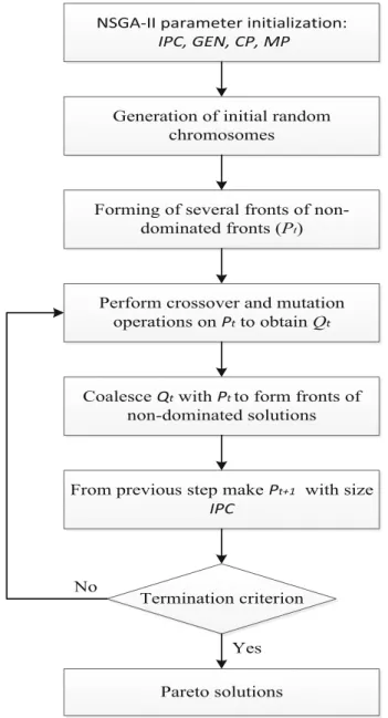
NSGA-II maintains a population of random individuals, which are improved over iter-ations. The improvement over iterations is represented in terms of the fitness value of the individual with respect to all the objectives of the problem. Each individual in a population is called as a chromosome and it represents an individual solution of the problem. Chromo-somes may be coded as binary or real value strings. The population is updated over iterations through a process of genetic operations of selection, cross-over and mutation. In crossover operation, two individuals or chromosomes exchange digits to form two new individuals or new chromosomes. In mutation, an individual is modified through string modification
oper-ations. In NSGA-II, we first create an offspring populationQt (of sizeN) from the parent
population Pt. Offspring population thus obtained is combined with parent population to
form an intermediate population of size 2N. The new population is obtained after updating
the existing population. In each iteration, the fitness of the individual is evaluated in terms of all the objectives. After evaluation of individuals in each generation, multiple individuals are selected through different selection mechanism. The detailed steps involved in NSGA-II
are schematically presented in Fig.2.
4.3 Implementation of NSGA-II
The detailed implementation of the algorithm to solve the current multi-objective model is discussed as follows.
4.3.1 Chromosome representation
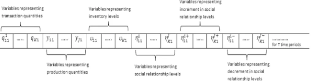
Each bit of the chromosome represents a decision variable described in Table2. The model
consists ofI suppliers, J retailers, K retailers, andT time periods. For a particular time
period, there would be a total of I× J transaction quantity variables between the
suppli-ers and the manufactursuppli-ers,J×K transaction quantity variables between the manufacturers
and the retailers, andK transaction variables representing the quantity sold by the retailers.
These transaction quantity variables are represented by the firstI×J+J×K+K bits of
the chromosome. The nextI+J bits of the chromosome represent the production quantity
variables ofIsuppliers andJmanufacturers. Similarly the nextI+J+K bits of the
chro-mosome represents the inventory variables ofIsuppliers,J manufacturers, andK retailers.
There would be a total ofI×Jsocial relationship level variables between the suppliers and
manufacturers, andJ×K social relationship level variables between the manufacturers and
retailers. These transaction quantity variables are represented by the nextI ×J +J×K
bits of the chromosome. The nextI × J +J ×K bits of the chromosome represent the
Generation of initial random chromosomes
NSGA-II parameter initialization:
IPC, GEN, CP, MP
Forming of several fronts of non-dominated fronts (Pt)
Perform crossover and mutation operations onPtto obtainQt
CoalesceQtwithPtto form fronts of non-dominated solutions
From previous step makePt+1 with size
IPC
Termination criterion
Pareto solutions Yes No
Fig. 2 Flow-chart of NSGA-II algorithm
the lastI×J+J×K bits of the chromosome represent the increment in the value of the
social relationship level at a particular time period. Hence, a total of
(I×J+J×K+K+I+J+I+J+K+I×J+J×K+I×J+J×K+I×J+J×K)
bits are used to represent the variables of one time period. Representing variables of all the time periods would require a chromosome of length
(I×J+J×K+K+I+J+I+J+K+I×J+J×K+I×J+J×K+I×J+J×K)×T
Fig. 3 Chromosome representation
of bits representing different variables in the chromosomes is not important. But an assumed fixed order is to be maintained throughout the population of chromosomes generated, so that when an optimal solution is generated in the form of a chromosome, it would be convenient to map the values of the bits of the chromosome to the variables. A sample representation of
chromosome is presented in Fig.3.
Initially a set of random chromosomes (Initial Population Count –IPC) are generated.
The algorithm is run for a specified number of generations (GEN), considering it as the
termination criterion.
4.3.2 Crossover operation
Since the encoded chromosomes consist of real values, in the current problem simu-lated binary crossover (SBX) has been used. The number of chromosomes participating
in crossover is controlled by crossover probability (CP). A detailed study on SBX can be
found inDeb(2001).
4.3.3 Mutation operation
A polynomial mutation is used to perform the mutation operation in NSGA II to solve the problem under consideration. The number of bits participating in mutation is controlled by
mutation probability (MP), which is a tuning parameter. A detailed study on polynomial
mutation can be found inDeb(2001).
There are four controllable parameters in NSGA-II: (1)IPC, (2)GEN, (3)CP, and (4)MP.
The quality of solution obtained depends largely on these four parameters. User defined these parameters and therefore there is a need to choose the optimal values for these parameters that yield better solutions. This can be achieved by tuning of parameters. Many parameter tuning approaches have been studied in literature, among them Taguchi method is vastly used for the analysis of robust design. In this research, Taguchi method of fractional factorial design has been implemented to obtain the optimal NSGA-II parameters. This method has
been discussed in the Sect.6.
5 An illustrative example and computational studies
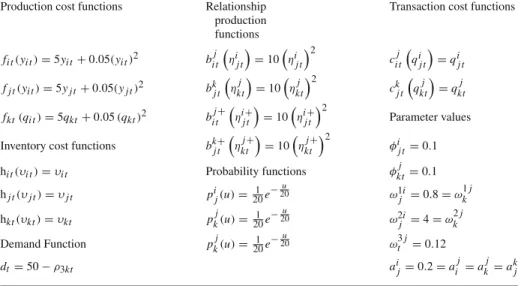
An illustrative example is presented and analysed using the above mentioned NSGA-II
algo-rithm. Most of the functions and parameters considered in this study are collected fromCruz
numer-Table 7 Functions and parameters used for computational study Production cost functions Relationship
production functions
Transaction cost functions
fi t(yi t)=5yi t+0.05(yi t)2 bi tj ηi j t =10ηij t2 ci tj qij t=qij t fj t(yi t)=5yj t+0.05(yj t)2 bkj t ηj kt =10ηktj2 ckj tqktj=qktj fkt(qi t)=5qkt+0.05(qkt)2 bi tj+ ηi+ j t =10ηij t+2 Parameter values Inventory cost functions bkj t+ηktj+=10ηktj+2 φij t=0.1 hi t(υi t)=υi t Probability functions φktj =0.1 hj t(υj t)=υj t pij(u)=201e− u 20 ω1i j =0.8=ω 1j k hkt(υkt)=υkt pkj(u)= 1 20e− u 20 ω2i j =4=ω 2j k Demand Function pkj(u)= 201e−20u ω3tj=0.12 dt=50−ρ3kt aij=0.2=a j i =a j k =akj
ical problem considers two suppliers(I =2), two manufacturers(J =2), and two retailers
(K =2), who trade for a term of five periods(T =5).
Suppliers primarily incur production costs and inventory holding costs for the given supply chain problem. Manufacturers incur costs related to transaction, supply disruption, oppor-tunism risks, and relationship maintenance and improvement in addition to production and inventory costs. Since, there is no production involved at the retailers, they mainly incur handling costs, inventory costs, costs related to transaction, supply disruption, opportunism risks, and relationship maintenance and improvement.
In this research, handling and fixed production costs are not considered and are assumed as sunk costs. Linear terms used for handling and production costs reflect the unit costs. The fact of increasing marginal production as the production quantity approaches the maximum capacity is reflected by the quadratic terms.
Analysis of this study has been carried out by solving four different variants of the problem: (1) profit versus risk, (2) profit versus emission, (3) emission versus risk, and (4) profit versus
risk versus emission. These analysis are presented in Sect.7followed by parameter setting
and Taguchi application in the next section.
6 Parameter tuning and application of Taguchi method
This section discusses Taguchi method implementation (Sadeghi et al. 2014) for NSGA-II
parameters setting in order to obtain the better quality solutions (with respect to objectives’ values) of the proposed SCN model. Fisher introduced factorial designs to investigate the effect of various factors on the mean response. In our context, factors are the parameters of algorithmic solution and response is the fitness value of the solution. In order to reduce large number of experiments in full factorial designs, Taguchi designed fractional factorial experiments. In Taguchi method the parameters affecting the solution are divided into two
be directly controlled. In order to reduce the variation around the target, Taguchi developed
a procedure to control the N factors. Analysis of results is performed in two ways: (1)
employing analysis of variance of experiments with a single replicate; (2) using signal to
noise ratio(S/N)in experiments with multiple replications. Owing to the better performance
of the second way (the one with multiple replications), solution in the current problem is
analysed usingS/N ratio. This method aims to minimize the effect of noise factors, in other
words the parameter setting at which the S/N ratio is maximum [effect of Signal (S) is much greater than effect of Noise (N)] is considered as the optimal.
6.1 Implementation of Taguchi method
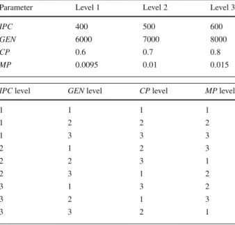
Four tuning parameters namely,IPC,GEN,CP, andMPof NSGA-II are considered as the
affecting parameters in Taguchi method. Three different levels of these parameters employed
for fractional factorial design are shown in Table8. These levels of the parameters have been
obtained using trial and error procedure. Tuning of parameters is carried out utilizing the
Taguchi L9orthogonal array shown in Table9.
Three different responses: (1) Pareto solution count (PSC), (2) spacing (Sp), and (3)
best solution (Bsol) (Deb 2001), each representing a specific quality of a solution obtained
using NSGA-II are considered as response variables for the experiments. To obtain the
Bsolin a replication, the fitness values of the solution are first normalized employing the
linear dimensionless approach of a multi-attribute decision making processes. Then they are summed together with a weight of 1/3 each. Since it is a minimization problem the solution with the lowest combined value of the normalized objective function values is considered as
the best. In case of a minimization problem, lower value ofSpand higher values ofPSCand
Bsolexplain better efficiency of NSGA-II.
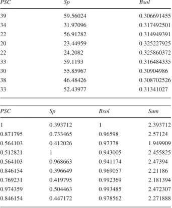
Three replications have been carried out for analysis. The results obtained for nine different
parameter settings (L9orthogonal array) in the first replication are displayed in Table10.
Table 8 Three different levels of parameters considered for parameter tuning
Parameter Level 1 Level 2 Level 3
IPC 400 500 600
GEN 6000 7000 8000
CP 0.6 0.7 0.8
MP 0.0095 0.01 0.015
Table 9 Nine different sets of
parameter setting IPClevel GENlevel CPlevel MPlevel
1 1 1 1 1 2 2 2 1 3 3 3 2 1 2 3 2 2 3 1 2 3 1 2 3 1 3 2 3 2 1 3 3 3 2 1
Table 10 Metrics obtained in the
first replication PSC Sp Bsol
39 59.56024 0.306691455 34 31.97096 0.317492501 22 56.91282 0.314949391 20 23.44959 0.325227925 22 24.2082 0.325860372 33 59.1193 0.316484335 30 55.85967 0.30904986 38 46.48426 0.308702526 33 52.43977 0.31341027
Table 11 Normalized metrics obtained in case of first replication PSC Sp Bsol Sum 1 0.393712 1 2.393712 0.871795 0.733465 0.96598 2.57124 0.564103 0.412026 0.97378 1.949909 0.512821 1 0.943005 2.455825 0.564103 0.968663 0.941174 2.47394 0.846154 0.396649 0.969057 2.21186 0.769231 0.419795 0.992369 2.181394 0.974359 0.504463 0.993485 2.472307 0.846154 0.447172 0.978562 2.271888
Table11shows the normalized values of responses, and the sum for each parameter setting.
These normalized values are obtained as follows.
ForPSC, normalized value of a parameter settingiis given by :
P SCi
max(P SC1,P SC2, . . . ,P SC9)
(32)
ForSp, normalized value of a parameter settingiis given by :
min(Sp1,Sp2, . . . ,Sp9) Spi
(33)
ForBsol, normalized value of a parameter settingiis given by :
min(Bsol1,Bsol2, . . . ,Bsol9) Bsoli
(34)
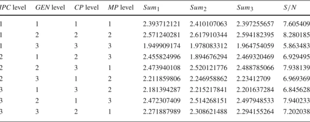
Sum values of all three replications are displayed in Table12. Since a solution with the
highest sum is desired, the aim is to find the maximumS/N calculated by
S/N = −Log10 1 n n i=1 1 sum2i (35)
wheren =3 represents the number of replications, andsumi represents the sum in theith
Table 12 Experimental results of three replications
IPClevel GENlevel CPlevel MPlevel Sum1 Sum2 Sum3 S/N
1 1 1 1 2.393712121 2.410107063 2.397255657 7.605409 1 2 2 2 2.571240281 2.617910344 2.594182395 8.280185 1 3 3 3 1.949909174 1.978083312 1.964754059 5.863483 2 1 2 3 2.455824996 1.894676294 2.469320469 6.929495 2 2 3 1 2.473940108 2.520121776 2.488785066 7.938139 2 3 1 2 2.211859806 2.246958862 2.23412709 6.969369 3 1 3 2 2.181394287 2.215217841 2.201637284 6.845628 3 2 1 3 2.472307409 2.514268151 2.497948533 7.940233 3 3 2 1 2.271887989 2.308621488 2.294155264 7.202038
Fig. 4 MeanS/Nplot for different levels ofIPC
7 7.5 8 1 2 3 Mean S/N IPC
Mean
S/N
vs.
IPC
Fig. 5 MeanS/Nplot for different levels ofGEN
6 6.5 7 7.5 8 8.5 9 1 2 3 Mean S/N GEN
Mean
S/N
vs.
GEN
Figures4,5,6and7display the graph of meanS/Nagainst the three levels ofIPC,GEN,
CP, andMP. The mean value ofS/N for a level jof the various parameters is calculated as
Fig. 6 MeanS/Nplot for different levels ofCP 6 6.5 7 7.5 8 1 2 3 Mean S/N CP
Mean
S/N
vs.
CP
Fig. 7 MeanS/Nplot for different levelsMP 6 6.5 7 7.5 8 1 2 3 Mean S/N MP
Mean
S/N
vs.
MP
mean(S/N)j = 1 3 ⎡ ⎣ i∈I PCj (S/N)i ⎤ ⎦ (36)whereI PCj represents the set of parameter combinations in which the level ofIPCis j.
mean(S/N)j = 1 3 ⎡ ⎣ i∈G E Nj (S/N)i ⎤ ⎦ (37)
whereG E Njrepresents the set of parameter combinations in which the level ofGENis j.
mean(S/N)j = 1 3 ⎡ ⎣ i∈C Pj (S/N)i ⎤ ⎦ (38)
whereC Pj represents the set of parameter combinations in which the level ofC Pis j.
mean(S/N)j = 1 3 ⎡ ⎣ i∈C Mj (S/N)i ⎤ ⎦ (39)
whereC Mj represents the set of parameter combinations in which the level ofC M is j.
Based on the highest mean values ofS/N, optimal NSGA-II parameters are obtained after
7 Results and discussion
In this section, illustrative example presented in Sect.4is solved by NSGA-II, where optimal
algorithmic parameters (IPC = 600, GEN = 7000, CP = 0.6,andMP = 0.0095) derived by
Taguchi method application in the above section, has been used. Next, we discuss the results obtained for four problem variants.
7.1 Problem 1: profit versus risk
We solve the proposed model considering three different cases with a view to examine the effectiveness of the parameters of relationship maintaining cost and risks on the decision policies. It is also aimed to answer the first three questions mentioned in the introduction section.
Case 1: the functions and parameters mentioned in Table7are used in this case. It can be observed that all the transaction costs and relationship costs are same between any pair of stakeholders of different tiers (i.e., between suppler and manufacturer; between manufacturer and retailer). Since profit maximization and risk minimization are conflicting objectives, our natural conscience would be to expect a Pareto-optimal relation between profit and risk.
Figure8shows a graph displaying the relationship between the risk and profit of the SCN.
It is evident from the graph that as risk decreases profit also decreases. This can be justi-fied by arguing that an increase in the level of social relationship requires investment in the form of time, additional personnel, money, etc. leading to decreased profit. This improve-ment in relationship level curtails the opportunism risks due to improved co-operation and communication between the tiers of supply chain. A firm chooses one solution among the Pareto-optimal front based on its profit preference and risk standards. One solution from the set of Pareto solutions, displaying data related to product flows, relationship level, demand
and inventories is shown in Table13.
It can be observed from Table13that social relationship level between each pair of
adja-cent echelon firm increases from 0 in period 1 to 0.429 in period 5, which means that social relationships become stronger over the periods. The increasing relationships curtail oppor-tunism risks leading to a decrease in overall risk in supply chain. The following observations
can also be made from Table13: product flow consistently increase from 2.909 to 3.865
200 250 300 350 400 450 500 900 1000 1100 1200 1300 Risk Profit