Level set segmentation of retinal structures

(1)

Level Set Segmentation of Retinal

Structures

Submitted by

Chuang Wang

for the degree of Doctor of Philosophy

of the

Department of Computer Science

Brunel University London

(2)

Declaration

I hereby declare that this thesis is solely completed by the candidate, Chuang Wang. The original research work has not been presented for the award of any other degree in the past. Some work in it has been published previously and that is stated in the text where relevant. All sources of material have been properly acknowledged and references have been provided.

(3)

List of Publications

Part of the work included in this thesis has been previously published in the following papers:

1. Chuang Wang, Yaxing Wang and Yongmin Li “Automatic Choroidal Layer Seg-mentation Using Markov Random Field And Level Set Method.”, (under review).

2. Chuang Wang and Yongmin Li “Blood Vessel Segmentation from Retinal Images Using the Level Set Method.” (under review).

3. Chuang Wang, Djibril Kaba and Yongmin Li “Level Set Segmentation of Optic Discs from Retinal Images.” Journal of Medical and Bioengineering, Vol. 4, No. 3, pp. 213-220, June 2015.

4. Chuang Wang, Yaxing Wang, Djibril Kaba, Zidong Wang, Xiaohui Liu and Yong-min Li, “Automated Layer Segmentation of 3D Macular Images Using Hybrid Methods.” The 8th International Conference on Image and Graphics (ICIG). Springer International Publishing, 2015, 614-628.

5. Chuang Wang, Yaxing Wang, Djibril Kaba, Haogang Zhu, Zidong Wang, Xiaohui Liu and Yongmin Li “Segmentation of Intra-retinal Layers in 3D Optic Nerve Head Images.” The 8th International Conference on Image and Graphics (ICIG), Springer International Publishing, 2015, 321-332.

(4)

Discs from Retinal Images.” International Conference on Biomedical and Bioin-formatics Engineering (ICBBE 2014).

The author of this thesis has also published the following papers during the PhD period, but the contents are not included in this thesis:

1. Djibril Kaba, Yaxing Wang, Chuang Wang, Yongmin Li, Xiaohui Liu, Haogang Zhu and Ana G. Salazar-Gonzalez “Retina Layer Segmentation Using Kernel Graph Cuts and Continuous Max-Flow.” Optics Express, 2015, 23(6): 7366-7584.

2. Djibril Kaba, Chuang Wang, Yongmin Li, Ana Salazar-Gonzalez, Xiaohui Liu, and Ahmed Serag. “Retinal blood vessels extraction using probabilistic mod-elling.” Health Information Science and Systems, 2, no. 1 (2014): 2.

(5)

(6)

Abstract

Changes in retinal structure are related to different eye diseases. Various retinal imaging techniques, such as fundus imaging and optical coherence tomography (OCT) imaging modalities, have been developed for non-intrusive ophthalmology diagnoses according to the vasculature changes. However, it is time consuming or even impossible for ophthalmologists to manually label all the retinal structures from fundus images and OCT images. Therefore, computer aided diagnosis system for retinal imaging plays an important role in the assessment of ophthalmologic diseases and cardiovascular disorders. The aim of this PhD thesis is to develop segmentation methods to extract clinically useful information from these retinal images, which are acquired from different imaging modalities. In other words, we built the segmentation methods to extract important structures from both 2D fundus images and 3D OCT images.

In the first part of my PhD project, two novel level set based methods were pro-posed for detecting the blood vessels and optic discs from fundus images. The first one integrates Chan-Vese’s energy minimizing active contour method with the edge con-straint term and Gaussian Mixture Model based term for blood vessels segmentation, while the second method combines the edge constraint term, the distance regularisation term and the shape-prior term for locating the optic disc. Both methods include the pre-processing stage, used for removing noise and enhancing the contrast between the object and the background.

Three automated layer segmentation methods were built for segmenting intra-retinal layers from 3D OCT macular and optic nerve head images in the second part of my PhD project. The first two methods combine different methods according to the data characteristics. First, eight boundaries of the intra-retinal layers were detected from the 3D OCT macular images and the thickness maps of the seven layers were pro-duced. Second, four boundaries of the intra-retinal layers were located from 3D optic nerve head images and the thickness maps of the Retinal Nerve Fiber Layer (RNFL) were plotted. Finally, the choroidal layer segmentation method based on the Level Set

(7)

framework was designed, which embedded with the distance regularisation term, edge constraint term and Markov Random Field modelled region term. The thickness map of the choroidal layer was calculated and shown.

(8)

Acknowledgement

I would like to thank my supervisor, Dr. Yongmin Li (Brunel University), for the guidance, support and patience throughout my PhD research and also appreciate his encouragement and carefulness while editing my papers. I could not finish my PhD on time without his guidance. I would also like to thank Djibril Kaba, Nick Rixon and Martin for proofreading drafts and providing suggestions and support. I would also like to thank the Department of Computer Science of Brunel University London for the funding of my research project.

Special thanks go to all the members of my PhD jury, Professor Steve Maybank (Department of Computer Science and Information Systems, Birkbeck, University of London), Dr. George Ghinea (Department of Computer Science, Brunel University) and Dr. Panos Louvieris (Department of Computer Science, Brunel University) who managed to take time off their busy schedules; go to all the lab members of Intelligent Data Analysis (IDA) group of the Department of Computer Science including Valeria Bo, Neda Trifonova, Moshina Ferdous, Miqing Li, Liang Hu, Izaz Rahman, Khalid Eltayef, Azerikatoa Ayoung, Hafedh Alrahbi and Almed Al-Madi, for friendship, inter-esting discussions and valuable comments through my PhD study.

Sincere thanks go to J.J. Staal and A. Hoover for publishing their retinal pho-tographs publicly; go to Dr. Yaxing Wang (Tongren Hospital, Beijing, China) and Haogang Zhu (Department of Optometry and Visual Science, City University, London, United Kingdom) for advices and providing the 3D retinal data both on macular and optic nerve head area. It is impossible to finish the work in the thesis without the data from these different institutes. I would like to thank Chunming Li et al. for providing the source code of the level set method, Quan Wang et al. for providing the source of the Markov Random Field method and Yuan Jing et al for providing the source of the continuous max-flow algorithm

Finally, a deep thanks to my parents, brother, sister-in-law (Xiaofeng Wang, Chungxia Huang, Qiang Wang and Peiqi Liao) and all the other relatives in my big family in China

(9)

(10)

List of Figures

1.1 The overview of my Ph.D. Work. . . 4

2.1 Schematic diagram of the cross-sectional view of eye and its major struc-tures copied from [eye, 2015]. The retina and choroid are the yellow tissue and reddish tissues with blood vessels inside, respectively. . . 10 2.2 Photograph of retina structures: blood vessels, optic disc, optic cup,

macula and fovea . . . 11 2.3 Illustration of ten cellular layers of the retina from Berne [Berne et al.,

2008]. . . 12 2.4 First human fundus image drawn by Van Trigt in 1853 [Van Trigt, 1853]. 15 2.5 Three different angle views of fundus images [Saine and Tyler, 2002]. . . 16 2.6 Some example images obtained from different fundus imaging techniques.

(A)Fluorescein Angiogram, (B) Scanning Laser Ophthalmoscopy, (C) Colour Fundus Photography, (D) Red-Free Photography, (E) Two reti-nal images taken from two different viewpoints for Stereo Fundus Pho-tography. . . 17 2.7 OCT scanner system schematic [Kraus et al., 2012]. Left: A-scan.

Backscattered intensity along the axial direction is measured and formed a single depth profile. Middle: B-scan. The OCT beam is measured in transverse direction. Right: Volumetric image. Multiple B-scans are acquired and formed into a 3D volumetric image. . . 19

(14)

2.8 The setup of the time domain OCT (TD-OCT) imaging system [Schu-man, 2008]. . . 20 2.9 The setup of the spectral domain OCT (SD-OCT) imaging system

[Schu-man, 2008]. . . 22 2.10 The SD-OCT example images captured by using the RTVue-100 system

around the ONH area. . . 23 2.11 The SD-OCT example images taken by using the Spectralis HRA+OCT

system around the macular area. . . 24 2.12 The SD-OCT example images taken by using the Spectralis HRA+OCT

system around the ONH area. . . 25 2.13 The setup of the swept source OCT (SS-OCT) imaging system

[Schu-man, 2008]. . . 26 2.14 Glaucomatous damage shown on fundus images [Gao et al., 2015]. (A)

Healthy fundus example, (B) Angle-closure Glaucoma fundus example, (C) Open-angle Glaucoma fundus example. . . 28 2.15 Some examples of fundus images which are affected by diabetes

retinopa-thy, including exudates, cotton-wool and drusen [Niemeijer et al., 2007]. 30 2.16 Some examples of AMD damage shown on B-scan macula and fundus

images [mac, 2015]. (A) Dry AMD example for both B-scan macular and fundus images, (B) Wet AMD example both on B-scan macula and fundus images. . . 32

3.1 Block diagram of the proposed blood vessel segmentation method. (a) The original retinal image. (b) The grey level image (Ig) of the original

image. (c) The closing operation of Ig (Ic). (d) The difference image

Id is obtained from the absolute difference between Ig and Ic. (e) The

matched filtering response of Id (Im). (f) Final output of the proposed

(15)

3.2 The DRIVE dataset: (a, d) Retinal images. (b, e) Our segmentation results. and (c, f) Ground truth image. . . 60 3.3 The STARE dataset (Normal): (a, d) Retinal images. (b, e) Our

seg-mentation results. and (c, f) Ground truth images. . . 60 3.4 The STARE dataset (Abnormal): (a, d) Retinal images. (b, e) Our

segmentation results. and (c, f) Ground truth images. . . 61

4.1 The process to locate the optic disc centre. (a) Rescaled image. (b) TheI

channel image. (c) Closing operation of I channel. (d) The template with the size of 201×201. (e) The Fourier correlated image. (f) The mask of rescaled image. (g) The border eroded image. (h) The convoluted image. (i) The optic disc centre located image. (j) The cropped image fromFrwith the size of 201×201. (k) The blood vessel segmented image.

(l) Open operation of vessel segmented image. (m) The optic disc centre reseted image. . . 68 4.2 Morphological close operation on the cropped retinal images. The first

row contains the input images, the second row contains the closed im-ages. . . 70 4.3 The DRIVE dataset: (a, d, g, j) The cropped retinal images. (b, e, h, k)

The optic disc centre reseted images. (c, f, i, l) Our segmentation results (Red is our segmentation result, blue is the ground truth). . . 79 4.4 The DIARETDB1 dataset: (a, d, g, j) The cropped retinal images. (b,

e, h, k) The optic disc centre reseted images. (c, f, i, l) Our segmentation results (Red is our segmentation result, blue is the ground truth). . . . 79 4.5 The DIARETDB0 dataset: (a, d, g, j) The cropped retinal images. (b,

e, h, k) The optic disc centre reseted images. (c, f, i, l) Our segmentation results (Red is our segmentation result, blue is the ground truth). . . . 79

(16)

5.1 Block diagram of retinal layers segmentation process. (NFL: Nerve Fiber Layer, GCL: Ganglion Cell Layer, IPL: Inner Plexiform Layer, INL: Inner Nuclear Layer, OPL: Outer Plexiform Layer, ONL: Outer Nuclear Layer, IS: Inner Segment, OS: Outer Segment, RPE: Retinal Pigment Epithelium) . . . 85 5.2 a) Original 3D macular image. b) The filtered image by nonlinear

anisotropic diffusion. c) The filtered image by ellipsoidal averaging. . . 86 5.3 a) The de-noised 3D macular image. b) The segmented object image. c)

The lower part of the segmented image across the IS boundary. d) The upper part of the segmented image across the IS boundary. . . 89 5.4 a) Graph construction for continuous max-flow and min cut with two

labels; b) Graph construction for max-flow and min-cut with n labels. . 90 5.5 Illustration of eight intra-retinal layers segmented result on an example

B-scan from top to bottom: 1. Vitreous, 2. NFL, 3. GCL-IPL, 4. INL, 5. OPL, 6.ONL-IS, 7. OS, 8. RPE, 9. Choroid. . . 96 5.6 Three examples of 3D visualisation of eight surfaces. . . 97 5.7 Twelve B-scan segmentation results from an example 3D segmented

mac-ular, (a)-(m) are10th, 30th, 50th, 70th, 90th, 110th, 130th, 150th,170th, 190th, 210th, 230th B-scans, respectively. . . 98 5.8 Examples of thickness maps of 7 retinal layers, layers exclude choroid

layer and total layers. The seven layers are 1. NFL, 2. GCL-IPL, 3. INL, 4.OPL, 5.ONL-IS, 6. OS, 7. RPE . . . 99

6.1 Block diagram of retinal layers segmentation process for 3D optic nerve head images. . . 103

(17)

6.2 Illustration of three intra-retinal layers segmented results of two cross-sectional B-scans from a 3D OCT optic nerve head image. (a) the 60th B-scan, which includes the optic disc region, (b) the 10th B-scan. Layer 1: retinal nerve fiber layer (RNFL), Layer 2 includes Ganglion Cell Layer, Inner Plexiform Layer, Inner Nuclear Layer and Outer Nuclear Layer (GCL, IPL, INL and ONL), Layer 3: retinal pigment epithelium layer (RPE). . . 109 6.3 Three examples of 3D OCT optic nerve head image layers segmentation

results. Four segmented layer surfaces of 3 different 3D images are vi-sualised in 3D. The shape of the surfaces are hypothesised to be related with eye diseases. . . 110 6.4 Ten B-scan segmentation results from an example 3D segmented optic

nerve head image, (a)-(k) are 10th, 20th, 30th, 40th, 50th, 60th, 70th, 80th, 90th, 100th B-scans, respectively. According to the segmentation results on B-scans from the 3D retinal images around the optic nerve head, the efficiency and accuracy of our method are shown. . . 111 6.5 The thickness maps of retinal nerve fiber layer (RNFL) from two 3D

optic nerve head image examples. The RNFL thickness map is useful in discriminating for glaucomatous eyes from normal eyes. (a) a healthy subject (b) a glaucomatous patient. . . 112

7.1 The challenge of the choroidal layer segmentation. (a) The original mac-ular B-scan. (b) The inhomogeneous texture from the B-scan. (c) The inseparable histogram distribution of the background and object from the B-scan. (d) The ground truth of the B-scan. . . 117 7.2 Block diagram of automatic choroidal layer segmentation. (a) The

orig-inal macular OCT image. (b) The de-noised OCT image by using the 3D anisotropic diffusion method. (c) The chopped OCT image. . . 119

(18)

7.3 The segmentation error of the bottom choroidal layer boundary of the dataset. (a) The signed mean and standard deviation(sd) difference between the ground truth and the proposed segmentation results for the bottom choroidal boundary (b) The unsigned mean and sd difference between the ground truth and the proposed segmentation results for the bottom choroidal boundary. . . 127 7.4 The Dice’s coefficient of the choroidal layer between the proposed method

and the ground truth. . . 128 7.5 The mean segmentation error of the bottom choroidal layer boundary

of the different methods, including the proposed method (A), GMM and MRF based Level Set Method (LSM) (B), MRF (C), Graph Cut method (D), Canny Edge detection (E), K-means algorithm (F), and Chan-Vese LSM (G). (a) The mean signed mean and standard deviation (sd) difference between the ground truth and the segmentation results (b) The mean unsigned mean and sd difference between the ground truth and the segmentation results. . . 128 7.6 The mean Dice’s coefficient of the choroidal layer between the

meth-ods and the ground truth, including the proposed method, GMM and MRF based LSM, MRF, Graph Cut, Canny Edge detection, K-means algorithms, and Chan-Vese LSM. . . 129 7.7 A choroid layer segmented example. (a)-(l) are the 10th, 30th, 50th,

70th, 90th, 110th, 130th, 150th,170th, 190th, 210th, 230th B-scans with the segmented choroidal bottom boundary marked in red, respectively. 129 7.8 Choroidal thickness map of the choroidal layer from this segmented

ex-ample. . . 130 7.9 3D view of the segmented choroidal bottom boundary from this example. 130

(19)

List of Tables

3.1 Performance of the segmentation methods on the DRIVE and STARE datasets . . . 57 3.2 Performance of vessel segmentation method on the STARE dataset

(nor-mal versus abnor(nor-mal images) . . . 58

4.1 The optic disc detection performance on the DRIVE, DIARETDB0 and DIARETDB1 datasets. . . 76 4.2 The optic disc segmentation performance on DRIVE, DIARETDB0 and

DIARETDB1 datasets. . . 78

5.1 Signed and unsigned mean and SD difference between the ground truth and the proposed segmentation results for the eight surfaces, respectively. 94 5.2 Average thickness of the 7 layers and overall of all the 30 volume images,

absolute thickness and relative thickness difference between the ground truth and the proposed segmentation results of the 7 layers and overall from all the data. . . 95

6.1 Signed and unsigned mean and SD difference between the ground truth and the proposed segmentation results for the four surfaces, respectively. 108

(20)

(21)

OCT Optical Coherence Tomography. DR Diabetes Retinopathy.

AMD Age-Related Macular Degeneration. DEM Diabetic Macular Edema.

CNV Choroidal Neovascularisation.

DRIVE Digital Retinal Images for Vessel Extraction. DIARETDB0 Diabetic Retinopathy Database 0.

DIARETDB1 Diabetic Retinopathy Database 1. STARE Structured Analysis of the Retina.

SD-OCT Spectral Domain Optical Coherence Tomography. MRF Markov Random Field.

HMRF Hidden Markov Random Field. LSM Level Set Method.

EM Expectation Maximisation. GMM Gaussian Mixture Model. HSI Hyper-spectral imaging.

SLO Scanning Laser Ophthalmoscope.

cSLO confocal Scanning Laser Ophthalmoscope. TD-OCT Time Domain Optical Coherence Tomography. CCD Charge-coupled device.

ONH Optic Nerve Head.

SS-OCT Swept- source Optical Coherence Tomography. IOP Intraocular pressure.

CDR Cup-to-disc ratio.

ALT Argon Laser Trabeculoplasty.

VEGF Vascular Endothelial Growth Factor. AREDS Age-Related Eye Disease Study. CVD Cardiovascular Diseases.

CHD Coronary Heart Diseases. NHS National Health Service. PAD Peripheral Arterial Disease. PVD Peripheral Vascular Disease. RHD Rheumatic Heart Disease. CHD Congenital Heart Disease.

(22)

DVT Deep Vein Thrombosis. k-NN k Nearest Neighbor. SDF Signed Distance Function.

CV Chan-Vese.

TPR True Positive Rate. FPR False Positive Rate. ACC Accuracy Rate.

RNFL Retinal Nerve Fibre Layer. FOV Field of view.

MAD Mean Absolute Distance. GCL Ganglion Cell Layer. IPL Inner Plexiform Layer. INL Inner Nuclear Layer. OPL Outer Plexiform Layer. ONL Outer Nuclear Layer.

IS Inner Segment.

OS Outer Segment.

REP Retinal Pigment Epithelium. WHO World Health Organisation. SD Standare deviation.

FT Fourier Transformation.

GT Ground Truth.

MLE Maximum Likelihood Estimators. MRI Magnetic Resonance Image. PCA Principle Component Analysis. RMSE Root-Mean Square Error. ROI Region of Interest. SVM Support Vector Machine.

(23)

Chapter 1

Introduction

Changes in the retinal structure, such as the area of the optic disc cup and optic disc, the thickness of retinal layers and so on, manifest many important eye diseases as well as systemic diseases, which originate either in the eye, the brain or the cardiovascular system. Much research in retinal structure analysis has been done to diagnose some of the most prevalent ocular diseases including glaucoma, diabetes, diabetic retinopathy, cardiovascular disease and age-related macular degeneration, most of which are common causes of irreversible blindness in the world. It is necessary and important to extract the retinal structure from retinal images, which are acquired from different imaging modalities, to assist the ophthalmologists in diagnosing eye diseases accurately and provide efficient treatment and management systems. In order to understand how retinal diseases affect the retinal structure, retinal structure analysis is introduced in Section 1.1. Section 1.2 introduces the aims of the Ph.D project. Finally, a thesis overview is briefly introduced in Section 1.3.

1.1 Retinal Structure Analysis

Retinal structure analysis has attracted more and more researchers and ophthalmolo-gists over the past 20 years. During this period retinal imaging technology has rapidly

(24)

1.1. Retinal Structure Analysis 1. Introduction

developed and enabled greater visibility of structures behind the retina and choroid. Retinal structure analysis has become an essential part of detecting and diagnosing eye diseases, and preventing loss of sight or blindness. Fundus imaging and optical coher-ence tomography (OCT) imaging modalities are two of the most widely used imaging systems in clinics and eye hospitals, used to aid ophthalmologists in obtaining a diag-nosis. Therefore, we mostly focus on retinal structure analysis using both the fundus images and OCT images.

Fundus imaging is an essential part of diagnosing and treating diabetic retinopathy (DR) and Age-related Macular Degeneration (AMD), which are the two most common forms of vision loss and blindness across the world. Almost all patients diagnosed with diabetes will develop diabetic retinopathy. AMD is the leading causes of vision loss among the elderly. It is non-reversible with undetectable early symptoms and eventu-ally may destroy sharp central vision. As diagnoses of diabetes are increasing and the percentage of the worlds’s elderly population is continuing to rise, both DR and AMD are becoming more serious health problems [Abr`amoff et al., 2010]. However, both dis-eases are manageable with a range of treatments available if patients are examined at least once a year [Ouyang et al., 2013]. The fundus image taken during such an exami-nation is analysed by ophthalmologists for signs of abnormality or further deterioration within the retina area. Based on the data analyse from the fundus images, diagnoses and treatments can be made and prescribed to the patient before the condition can deteriorate beyond a state where it can be managed.

Fundus photography can be used to diagnose other medical conditions in the body [Abr`amoff et al., 2010]. Often, cardiovascular conditions such as stroke, myocardial infarction and hypertension can change the structure of the retina, affecting the di-ameter of retinal arterioles and venules [Wong et al., 2004]. For example, when the ratio of the diameters of arterioles and venules becomes unbalanced, this can indicate an abnormality in the arterioles and venules, which is often associated with myocar-dial infarction. The ability to view such abnormalities from fundus images by using

(25)

some retinal structure analysis tools can help to detect symptoms and diagnose the dis-eases earlier, enabling proper treatment to prevent deterioration or even non-reversible blindness.

OCT imaging provides more information about the retinal morphology, which makes it possible for this imaging technique to be used for close monitoring of reti-nal status and guidance of retireti-nal treatment strategies [Abr`amoff et al., 2010]. OCT imaging is successfully used as an image guided diagnosis and treatment system in ophthalmology, especially in diabetic macular edema (DME) and choroidal neovascu-larization. DME is a form of diabetic retinopathy, while choroidal neovascularization (CNV) is the wet form of age related macular degeneration. The DME causes vision loss through fluid leakage into the macula. By using the OCT imaging technology, the thickness of the central retina can be measured and used as an important indicator for diagnosing DME [Murakami and Yoshimura, 2013]. CNV is the creation of new blood vessels in the choroid layer which can rupture and bleed because they are weaker than normal blood vessels. The CNV may produce extreme myopia, myopic degeneration, or age-related developments, which may cause a sudden degeneration of central vision. The parameters of the cystoid spaces, diffuse intra-retinal fluid, retinal fluid, sub-retinal hyper-reflective material, or a change of fluid measured from OCT images is important to indicate CNV [Mokwa et al., 2013].

OCT photography is widely used to diagnose glaucoma, which is the second most common cause of blindness all over the world [Resnikoff et al., 2004]. The structural changes in the optic nerve head and retinal nerve fiber layer are measured from OCT images for early glaucoma diagnosis and aid in providing proper treatment to prevent visual loss. The cup-to-disc ratio calculated from 3D optic nerve head OCT images is an important indicator for glaucoma. The thickness of the retinal nerve fiber layer is calculated for aiding a glaucoma diagnosis.

Retinal structure analysis is increasingly important in clinical applications for as-sisting ophthalmologists in diagnosing eye diseases, especially during early diagnosis

(26)

Figure 1.1: The overview of my Ph.D. Work.

and management for eye diseases. The aim of my Ph.D project is to build a structure analysis tool for extracting important retinal structures from both 2D and 3D retinal images, which are obtained from different imaging modalities including fundus cameras and OCT imaging systems, for assisting ophthalmologists in diagnosing eye diseases and providing the proper treatment strategies in advance to prevent serious deterio-ration. Figure 1.1 shows the framework of this Ph.D project. The first part of this project mainly focused on fundus image analysis to segment out the blood vessels and optic discs. The second part of this project focused on OCT image analysis, and the images involved in this project are acquired from two different imaging modalities and taken around different retinal areas including the optic nerve head area and macular area.

(27)

1.2. Aims and Objectives 1. Introduction

1.2 Aims and Objectives

Retinal imaging technology has developed dramatically during the last few decades. This has enabled ophthalmologists to capture a clearer view of the structure and tissues of the retina or even the choroid. However, it is time consuming or even impossible to hand label all the retinal structures to detect the tiny changes in the captured images. Therefore, the aim of this thesis is to develop retinal image analysis tools for images obtained from different imaging modalities. The tools are used to detect the retinal structure changes and extract useful information, which enable ophthalmologists to precisely diagnose diseases especially in their early stages and give proper treatment to prevent future deterioration.

The specific objectives of the Ph.D. project, as described in this thesis, are sum-marised as follows:

• Blood vessels: Develop an automated segmentation method for extracting blood vessels from retinal images and evaluate the performance of the segmentation us-ing two public datasets DRIVE and STARE.

• Optic disc: Develop an automated optic disc segmentation method for retinal images and evaluate the performance of the segmentation method using three public datasets DRIVE, DIARETDB0 and DIARETDB1.

• Macular: Develop a fully automated segmentation method for extracting seven intra-retinal layers from 3D macular images and evaluate the performance of this method using a dataset collected from Tongren Hospital, Beijing, China by using the imaging modality SD-OCT Spectralis HRA+OCT (Heidelberg Engineering, Germany).

• Optic nerve head: Develop a method for intra-retinal layers segmentation from 3D optic nerve head images and evaluate the performance of the method on images obtained from Moorfield Eye Hospital by using the imaging modality

(28)

1.3. Thesis Overview 1. Introduction

RTVue-100 SD-OCT (Optovue, Fremont, CA, USA).

• Choroidal layer: Develop a method for detecting the choroidal layer from 3D macular images and validate the performance of the method through a dataset from Tongren Hospital by using the imaging modality SD-OCT Spectralis HRA+OCT (Heidelberg Engineering, Germany).

1.3 Thesis Overview

This thesis includes 8 chapters. The rest of the thesis is organised as follows:

• Chapter 2 provides some relevant background and explains the major challenges of this project. It includes an introduction to the anatomy of the eye. This is fol-lowed by a describtion of the fundus and Optical Coherence Tomography (OCT) imaging techniques. Then, some of the most prevalent retinal diseases includ-ing glaucoma, diabetes, diabetes retinopathy, age-related macular degeneration, and cardiovascular disease are discussed. Two classical models of the level set method are discussed. Finally, some major topics and challenges in fundus and OCT image analysis are described.

• Chapter 3 describes an automated and unsupervised blood vessel segmenta-tion method from fundus images by using the level set method, which combines Chan-Vese’s region based term with the Gaussian Mixture term and distance reg-ularisation term. The morphological closing operation and matched filtering are used as a preprocessing process to keep the vessels inside the optic disc, remove the noise of the optic disc boundary, and enhance the blood vessel information. The proposed method is tested and compared with the state-of-the-art meth-ods on two public datasets namely DRIVE and STARE. It achieves an average accuracy greater than 95%.

(29)

from digital fundus images. The template matching method is used to approx-imately locate the optic disc centre, and the blood vessels are extracted to re-located the centre of the optic disc. This is followed by applying the level set method, which incorporates the edge term, distance regularization term and shape-prior term, to segment the shape of the optic disc. Seven measurements are used to evaluate and compare the performance of our proposed methods with the state-of-the-art methods on three public datasets: DRIVE, DIARETDB0 and DIARETDB1.

• Chapter 5 presents an automated segmentation method to detect intra-retinal layers in OCT macular images acquired from a high resolution SD-OCT Spec-tralis HRA+OCT (Heidelberg Engineering, Germany). The algorithm starts by removing all the OCT imaging artifects including the speckle noise and enhances the contrast between layers using both 3D nonlinear anisotropic and ellipsoid av-eraging filers. Eight intra-retinal boundaries of the retina are detected by using a hybrid method which combines the hysteresis thresholding method, level set method, and multi-region continuous max-flow approaches.

• Chapter 6introduces an intra-retinal layer segmentation method from SD-OCT images around the optic nerve head acquired from a high resolution RTVue-100 SD-OCT (Optovue, Fremont, CA, USA). This method starts by removing all the OCT imaging artifects including the speckle noise and enhances the contrast between layers using the 3D nonlinear anisotropic diffusion filter. Afterwards, we combine the level set method, k-means and Hidden Markov Random Field (HMRF) method to segment four surfaces of the retinal images around optical nerve head.

• Chapter 7 presents a choroidal layer segmentation method from 3D macular images by using the level set method, which adopts the Markov Random Feld term with the distance regularisation and edge constraint terms. Before that, the

(30)

3D nonlinear anisotropic diffusion filter is used to remove all background noise. The segmented results are compared with the manual segmented cross-sectional B-scans. The experimental results show that our method can accurately estimate the choroidal boundary.

• Chapter 8provides conclusions for this Ph.D project in this thesis and highlights some potential future research directions under investigation.

(31)

Chapter 2

Background

This chapter describes the background of this Ph.D. project. In order to understand the structure of the eye, Section 2.1 briefly discusses the eye anatomy. Some typical retinal diseases are introduced in Section 2.2. This is followed by a description of the retinal imaging techniques in Section 2.3. A simple discussion of the retinal image analysis is given in Section 2.4. Two famous level set models are introduced in Section 2.5.

2.1 Eye Anatomy

It is important to understand the structure and functions of the eye to help the diagnosis and treatment of eye diseases. The diagram of the cross-sectional view of the eye and its major structures [eye, 2015] is shown in Figure 2.1. The eye works similar to a camera with many parts of the eye working together to produce clear vision. The white part of the eye is called the sclera, which is used to protect the eyeball. The black dot at the centre of the eye through which the light enters the eye is called the pupil. The coloured iris, which is brown, green, blue or a mix of these colours is part of the eye, and surrounds the pupil and adjusts the size of the pupil to control the amount of light entering the eye. The curved shape of the cornea is the “front window”of the

(32)

2.1. Eye Anatomy 2. Background

Figure 2.1: Schematic diagram of the cross-sectional view of eye and its major structures copied from [eye, 2015]. The retina and choroid are the yellow tissue and reddish tissues with blood vessels inside, respectively.

eye and transmits and focuses light onto the lens underneath. The curve of the cornea can determine if someone has near or long sight as well as other vision impairments. Corrective laser surgery works by reshaping the cornea to change the focus.

The lens is located behind the pupil and acts similarly to a camera lens by focusing light onto the retina. The retina is the yellow part of the eye and contains two types of photoreceptor: rods and cones. There are approximately 6 million cones within the macula area of the retina and are the most densely spaced together in the Fovea. Cones primarily process light and colour. Rods are positioned in the outer edge of retina and are responsible for sight during low light and peripheral vision. Through the photoreceptor cells, the retina absorbs and converts light to electrical impulses, which are transferred to the brain along the optic nerve. The optic nerve is located in the centre of the retina. The choroid is located between the retina and the sclera and

(33)

provides oxygen and nourishment to the retina.

Figure 2.2: Photograph of retina structures: blood vessels, optic disc, optic cup, macula and fovea

Figure 2.2 shows the digital fundus image with retinal structures marked, which includes retinal blood vessels, the optic disc, and macula. The macula area is the dark region located roughly at the centre of the retina, which is responsible for the vision needed for daily activities such as reading and writing. At the centre of the macula is the fovea, which contains the greatest concentration of cone cells in the eye. The fovea is responsible for central, sharp vision and is necessary for reading, driving and other activities. The optic disc is the visible part located at the front of the optic nerve, which is known as the blind spot because it contains no rods and cones. The optic cup is located at the centre of the optic disc. The ratio between the diameter of the optic

(34)

cup and the diameter of the optic disc is important in the diagnosis of glaucoma.

Figure 2.3: Illustration of ten cellular layers of the retina from Berne [Berne et al., 2008].

Ten cellular layers of the retina from [Berne et al., 2008] are illustrated in Figure 2.3. The retina is divided into the following layers:

1. The pigment epithelium: the main function is to maintain the quality of an image through absorbing the stray light and preventing scatter;

2. Photoreceptor layer: composed of photoreceptor (rods and cones), which receive light from a particular part of the visual field;

3. The external limiting membrane: it forms intercellular connections with the pho-toreceptors, M¨uller cells and photoreceptors;

(35)

2.2. Retinal Imaging Techniques 2. Background

4. The outer nuclear layer: it includes the cell bodies of rods and cones;

5. The outer plexiform layer: formed of the synapses between the photoreceptors (rods and cones) and retinal horizontal and bipolar cells;

6. The inner nuclear layer: made up of the nuclei, cell bodies of the horizontal cells, the bipolar cells and M¨uller cells;

7. The inner plexiform layer: the synaptic formation between the bipolar cells axons and ganglion cells dendrites;

8. The ganglion cell layer: formed by the cell bodies of the ganglion cells;

9. The retinal nerve fibre layer: composed of axons of the ganglion cells, through which the electrical impulses are transmitted to the visual cortex;

10. The inner limiting membrane: it contains the M¨uller cells and is located within the innermost layer of the retina.

Below the retina is the choroid, which supplies blood to the retina. The structure of the choroid consists of the following layers:

1. The Bruch’s membrane: separates the choroid from retina;

2. The choriocapillaris;

3. The Sattler’s layer: contains the medium diameter blood vessels;

4. The Haller’s layer: composed of larger diameter blood vessels and is located at the outermost layer of the choroid.

2.2 Retinal Imaging Techniques

Retinal imaging is used by optometrists to take pictures of the retina, blood vessels and the optic nerve inside of the eye. These pictures help ophthalmologists to diagnose and

(36)

manage eye diseases including glaucoma, diabetes, macular degeneration and so on. This method is a non-invasive imaging technique, which captures a more detailed view of inside of the eye compared to conventional methods. Retinal disorders are detected in their early stages by using retinal imaging techniques. This early detection makes it possible to prevent serious disease progression or even vision loss. Retinal images are captured and stored giving a permanent and historical record of the eye, and make it easier for ophthalmologists to discover minor changes in the eye by comparing images taken over time. Nowadays, retinal imaging modalities, such as fundus photography and optical coherence tomography (OCT) machines, are widely used in clinics. Fundus imaging techniques are widely used to detect eye diseases including diabetic retinopa-thy, glaucoma, and age-related macular degeneration, while OCT imaging techniques are famous for diagnosing and managing patients with diabetic retinopathy, macular degeneration, and inflammatory retinal diseases [Abr`amoff et al., 2010].

2.2.1 Fundus Imaging

The Dutch ophthalmologist Van Trigt drew the first fundus image in 1853 [Van Trigt, 1853] as shown in Figure 2.4. Fundus photography was invented in the 1920’s and has been widely used since the 1960’s [Gramatikov, 2014]. Fundus photographs are used to detect medical signs, such as hemorrhages exudates, cotton wool spots, blood vessel abnormalities, and pigmentation. Fundus imaging is one of the most widely used imaging tools in clinics.

Fundus photography uses a fundus camera to capture retinal images of the interior surface of the eye. A fundus camera is installed with a low power microscope which provides a magnified view of the retina. A fundus image obtained from the camera provides 2-D representative image of 3-D retina by using reflected light. The typical width of the camera view is from 30 to 50 degrees. The whole imaging process takes around 5 to 10 minutes. Figure 2.5 shows fundus images with three different widths of view: 20, 40, 60 degrees, respectively [Saine and Tyler, 2002].

(37)

Figure 2.4: First human fundus image drawn by Van Trigt in 1853 [Van Trigt, 1853].

The broad category of fundus imaging contains the following modalities [Abr`amoff et al., 2010]:

1. Fundus photography (including red-free photography): A filter is used to select specific colours from the imaging lights to enhance the appearance of specific areas of the retina. Red-free photography is used to highlight the blood vessels by removing the red colour. An example image is shown in Figure 2.6(D).

2. Colour fundus photography: Provides a full colour fundus image, Figure 2.6(C) shows an example of a colour fundus image.

3. Stereo fundus photography: Two images of the same retina are taken from two different viewpoints and fused to obtain a virtual, depth-enhanced stereo image,

(38)

Figure 2.5: Three different angle views of fundus images [Saine and Tyler, 2002].

which helps the physician study the patient’s retina more easily and compre-hensively. Two retinal images taken from different angles are shown in Figure 2.6(E).

4. Hyper-spectral imaging (HSI): Used to obtain an electromagnetic spectrum for each pixel in the image, which can be used to record subtle variations of spectral properties, for finding objects, identifying materials, or detecting processes. It is widely used for analysing the spectra of inhomogeneous materials that contain a wide range of spectral and spatial information [Park et al., 2006]. The

(39)

hyper-2.2. Retinal Imaging Techniques 2. Background

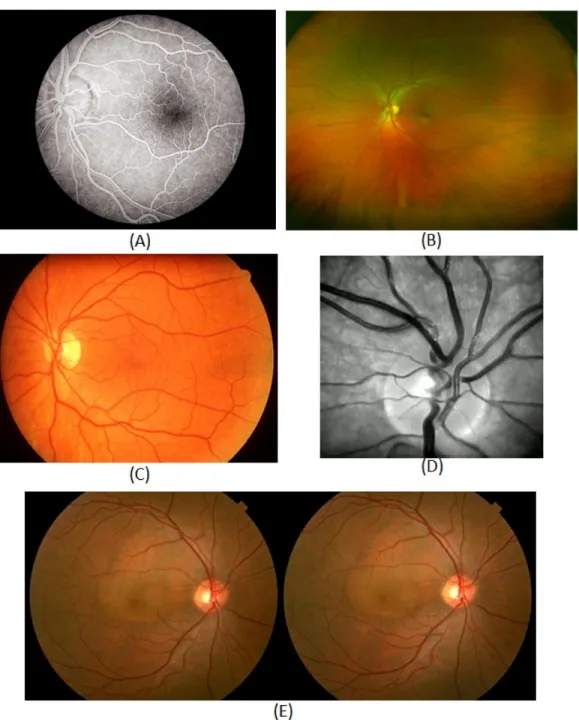
Figure 2.6: Some example images obtained from different fundus imaging techniques. (A)Fluorescein Angiogram, (B) Scanning Laser Ophthalmoscopy, (C) Colour Fundus Photography, (D) Red-Free Photography, (E) Two retinal images taken from two dif-ferent viewpoints for Stereo Fundus Photography.

spectral camera detects the consumption of the oxygen in the retina, which is used to diagnose diseases including hemorrhagic shock, peripheral artery disease,

(40)

diabetes and many other abnormalities [Gramatikov, 2014].

5. Scanning laser ophthalmoscopy (SLO): Provides a high quality television image of any specific area of the retina by utilising horizontal and vertical scanning mirrors. This technique is widely used for diagnosing eye disorders, such as glaucoma, macular degeneration and other retinal pathologies. Figure 2.6(B) shows an example SLO image.

6. Adaptive optics SLO: Used to measure living retinal cellular and sub-cellular structures in the human eye to help diagnose retinal disorders [Huang et al., 2012]. It provides a high resolution image of a specific region of interest on the retina with adaptive optics technology, which is used to reduce the effect of wavefront distortions.

7. Fluorescein angiography: Require the injection of a small amount of dye into a vein at the bend of the elbow. After that, a specialised camera is used for imaging the blood flow in the retina and choroid. Because fluorescein angiography obtains images with high contrast between the blood vessel and background, it can be used to accurately detect and quantify the geometric changes in blood vessels. However, this technique is not available for all patients because of allergic reactions. Fluorescein angiography is normally used for the diagnosis of the eye disorders, such as: macular degeneration, and diabetic retinopathy. An example image of fluorescein angiography is shown in Figure 2.6(A).

2.2.2 Optical Coherence Tomography (OCT) Imaging

OCT is a non-invasive technology used to obtain high resolution, cross-sectional images of the microstructure of the eye. OCT was designed by Fujimoto’s group at MIT in 1991 and was first introduced commercially in 1996 [Huang et al., 1991]. OCT uses light to scan in a similar way to an ultrasound scan. An OCT scan generally shows much finer detail than an ultrasound scan. However, ultrasound can be used to scan

(41)

deeper into tissue and through structures that are opaque to light [Fujimoto et al., 2000]. OCT is used to see details of the cornea or the retina, while ultrasound is used to see structures hidden by the iris. A near infrared low intensity light is directed into the retina of the patient. The light that is reflected back is captured by the OCT modality’s detectors and converted into a high resolution cross-sectional image of the internal microstructure of the retina, displaying the different intra-retinal layers. The different layers of the retina reflect the light back at different frequencies. This allows the different layers to be seen.

Figure 2.7: OCT scanner system schematic [Kraus et al., 2012]. Left: A-scan. Backscattered intensity along the axial direction is measured and formed a single depth profile. Middle: B-scan. The OCT beam is measured in transverse direction. Right: Volumetric image. Multiple B-scans are acquired and formed into a 3D volumetric image.

This imaging technique has been used to diagnose and manage many retinal disor-ders including glaucoma, choroidal neovascularization, macular edema, vitreomacular traction and diabetic retinopathy [Jaffe and Caprioli, 2004]. The main advantage of this technique in medical applications is that it is possible to image tissue structure on

(42)

site and in real time. There are three main OCT imaging techniques developed to cap-ture cross-sectional or volumetric images of retina. An image scanned along the depth direction of the retina is called A-scan as Figure 2.7 (Left). Several A-scans across the area of the tissue can be collected together and used to create one cross sectional image which is called a B-scan as Figure 2.7 (Middle). A 3D image can be created using a collection of B-scans in parallel Figure 2.7 (Right).

Time-domain OCT (TD-OCT)

Figure 2.8: The setup of the time domain OCT (TD-OCT) imaging system [Schuman, 2008].

The TD-OCT technique is frequently compared to ultrasound due to the similarity in technique. TD-OCT technique uses the backscattered echo time delay and light intensity levels to create a cross-sectional image. TD-OCT has around 10µm axial resolution, which is much higher than ultrasound at around 150µm. TD-OCT modality captures around 400 axial scans per second. The traditional OCT method (TD-OCT)

(43)

is used to represent the location of each reflection within the position of a moving reference mirror in the time information [Huang et al., 1991]. The StratusOCT (Carl Zeiss Meditec Inc., Dublin, CA, USA) is one of the most widely used TD-OCT devices in clinical applications. It acquires 400 A-scans per second with an axial resolution of 10 µm. The highest lateral resolution is up to around 20µm.

Figure 2.8 shows the time-domain OCT (TD-OCT) imaging system setup [Schuman, 2008]. TD-OCT works by shining light from a light source, such as a superluminescent diode (superluminescent diodes operate on a bandwidth of around 20 to 50 nanometers) or a broad bandwidth laser into a beam splitter (fiber coupler). This splits the light into two beams, with one going to the mirror on the reference arm, and one going to the mirror on the sample arm which can be adjusted to localise the depth of scan into the tissue. Some light from the sample arm mirror is reflected back off the eye tissue but most of it scatters away in different angles. Light from the sample and reference mirrors then travels back to the beam splitter. If the sample and reference lights are coherent, meaning that the light depths of the sample and reference mirrors are the same, a combination of both reflections of light produces an interference pattern that is processed by the photodetector to produce an image or an A-scan [Huang et al., 1991]. If the sample and reference light are incoherent, they will not produce an interference pattern that can be converted to an image. It is difficult to precisely image retinal tissue in three dimensions because of eye movement.

Spectral-domain OCT (SD-OCT)

Although fundamentally similar to TD-OCT, SD-OCT has some significant variations. SD-OCT systems are able to scan and perform imaging at a higher speed and scan depth, and are able to take thousands of A-scans a second. Both TD-OCT and SD-OCT use a central wavelength range of approximately 800 to 1100 nm. Figure 2.13 shows a schematic of spectral domain OCT (SD-OCT) imaging system setup. One of the main differences is that the reference mirror is in a fixed position in SD-OCT. The

(44)

adjustments of the referencing mirror used in TD-OCT are not efficient and limit in the speed and sensitivity of the scans. It is faster and more efficient to detect reflections from the entire range of depths simultaneously. Therefore, in SD-OCT the reference mirror is kept stationary, and the interference between the sample and reference beams is detected as a spectrum. The interference pattern is split using a grating diffraction into its frequency components and all of these components are simultaneously detected by a charge-coupled device (CCD) camera. The CCD camera is sensitive to several different frequencies.

Figure 2.9: The setup of the spectral domain OCT (SD-OCT) imaging system [Schu-man, 2008].

SD-OCT machines are up to 40 to 110 times faster than TD-OCT machines [Schu-man, 2008]. This faster speed allows for a more rapid capturing of B-scans, and for a higher level of precision when modelling and visualising 3D datasets. However, TD-OCT is only be able to reach a maximum of around 512 A-scans. Images from B-scans can be presented as grey scale or false colour images. Greyscale images are usually preferable for identifying fine detail, for example, the differences in the layers of the

(45)

retinal microstructure. In false colour images, bright colours such as red or white rep-resent areas of high reflectivity, while darker colours such as blue or black reprep-resent areas where the reflections are minimal or nonexistent.

Figure 2.10: The SD-OCT example images captured by using the RTVue-100 system around the ONH area.

RTVue-100 (Optovue, Fremont, CA, USA) system is one example of a SD-OCT imaging system with high speed image capture (26,000 A-scans per second). It achieves up to 5µmaxial resolution, which is two times higher resolution than the StratusOCT (Carl Zeiss Meditec Inc., Dublin, CA, USA) system. This system can obtain a 3D optic nerve head (ONH) image with 16 bits per pixel and 101 B-scans, 513 A-scans, 768 pixels in depth. An example 3D image acquired by using RTVue-100 system around the optic nerve head (ONH) area is shown in Figure 2.10. Figure 2.10 (A) shows the ONH SD-OCT volume, Figures 2.10 (B)-(D) show the reduced volumes of the original ONH volume in X, Y, Z direction. Figures 2.10 (E)-(O) are the 1st, 10th, 20th, 30th,

(46)

40th, 50th, 60th, 70th, 80th, 90th, 100th scans from the ONH volume, respectively. Figures 2.10 (P) and (Q) are the colour and the grey level en face images.

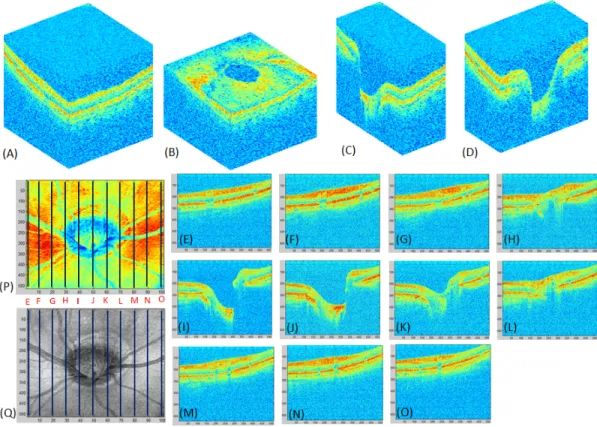
Figure 2.11: The SD-OCT example images taken by using the Spectralis HRA+OCT system around the macular area.

Spectralis HRA+OCT (Heidelberg Engineering, Germany) is another example of a SD-OCT system. It acquires up to 40,000 A-scans per second for a 3D image. It achieves up to 3.9µm axial resolution, 7µm depth resolution and 14µm lateral reso-lution. This imaging system has been widely used to diagnose retinal diseases, which provides 3D image with 256 B-scans, 512 A-scans, 992 pixels in depth and 16 bits per pixel. Figures 2.11 and 2.12 show example volume images of SD-OCT Spectralis HRA+OCT around the macula and ONH, respectively. Figure 2.11 (A) shows the example macular OCT volume, Figures 2.11 (B)-(D) show the reduced macula SD-OCT volumes in X, Y, Z direction. Figures 2.11 (E)-(O) are the 1st, 25th, 50th, 75th, 100th, 125th, 150th, 175th, 200th, 225th, 250th scans from the ONH volume,

(47)

respec-2.2. Retinal Imaging Techniques 2. Background

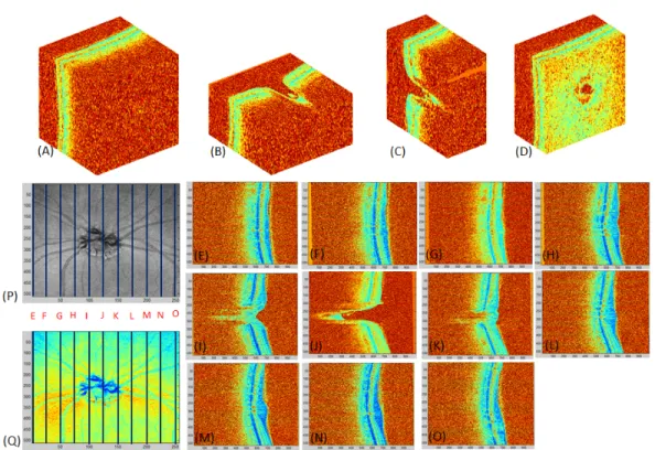
Figure 2.12: The SD-OCT example images taken by using the Spectralis HRA+OCT system around the ONH area.

tively. The grey level and colour en face images of the macular volume are shown in Figures 2.11 (P) and (Q) respectively. An example ONH volume captured by using the Spectralis HRA+OCT system is shown in 2.12 (A). The reduced volumes of the ONH volume in X, Y, Z direction are shown in Figures 2.12 (B)-(D), respectively. The 1st, 25th, 50th, 75th, 100th, 125th, 150th, 175th, 200th, 225th, 250th scans captured from the ONH volume are shown in Figures 2.12 (E)-(O), respectively. Figure 2.12 (P) and (Q) are the grey level and colour en face images.

Swept-source OCT (SS-OCT)

Swept-source OCT (SS-OCT) is the latest form of OCT. Because previous forms of OCT technologies do not have the ability to view deeply or clearly enough into the eye tissues, the primary function and development of SS-OCT is to enable a clearer and deeper view into the eye, gaining the ability to visualise the choroid. SS-OCT employs

(48)

a fast wavelength scanning light source such as laser rather than a low-coherence light source compared to TD-OCT and SD-OCT [Lim et al., 2014].

Figure 2.13: The setup of the swept source OCT (SS-OCT) imaging system [Schuman, 2008].

The setup of the swept-source OCT imaging system is shown in Figure 2.13 [Schu-man, 2008]. Instead of using a spectrometer and a CCD camera to detect the inter-ference signal in SD-OCT technology, a frequency swept laser source and a high speed photodetector are used to detect the interference signal. The reflections from the scan-ning mirror and reference mirror are detected by a single photodetector, which greatly increases the scanning speed and reduces the cost because the photodetector is much cheaper and simpler than a CCD camera [Schuman, 2008]. By using the swept source, the SS-OCT system is able to provide faster scanning speeds, uniform image quality and improved vitreous visualisation. Furthermore, the SS-OCT adopts longer wavelengths

(49)

2.3. Retinal Diseases 2. Background

(1050 nm) which increase tissue penetration, reduce intra-tissue light scattering, and make it possible to see the optic nerve and macula on the same scan.

DRI OCT-1 Atlantis (Topcon, Tokyo, Japan) is one example of a SS-OCT system. It provides 100,000 A-scans per second with 1,050nmwavelength, which is the fastest scanning speed in the world [Schuman, 2008]. It enables the viewing of deep eye tissues such as choroid and sclera within a very short time. This system achieves a high resolution with 20µm lateral resolution and 8µm in-depth resolution.

2.3 Retinal Diseases

The retina is the light sensitive tissue which is responsible for vision. It is located on the inside back wall of the eye. The retina are vulnerable to diseases, including glaucoma, diabetes retinopathy, age-related macular degeneration, cardiovascular diseases and other inherited retinal degenerations. Some of the diseases can lead to visual loss or permanent blindness. Some of the most prevalent retinal diseases are briefly introduced in the following.

2.3.1 Glaucoma

Glaucoma affects the optic nerve of the eye. It increases the pressure in the eye because the extra eye fluid (Aqueous Humour) flows though an area of the sclera known as the Trabecular Meshwork and disrupts this area [Quigley and Broman, 2006]. Glaucoma is the second highest cause of permanent blindness [Thylefors et al., 1995]. The eye regu-lates the necessary drainage of fluid through the Trabecular Meshwork. This pressure is known as Intra Ocular Pressure (IOP). Although people with a high IOP may not necessarily go on to develop Glaucoma, sufferers do tend to have a higher level of IOP which may often be hereditary. Glaucoma is typically without symptoms until later in life. These affected are usually 40 and over. The symptoms of Glaucoma are: gradual loss of peripheral vision leading to tunnel vision.

(50)

There are two main types of Glaucoma: Open-angle Glaucoma and Angle-closure Glaucoma. Figure 2.14 compares the two types of Glaucomatous fundus images with the image of a healthy fundus. The cup-to-disc ratio (CDR) is measured to diagnose and track the progression of glaucoma. This ratio is calculated by comparing the diameter of the optic cup with the diameter of the optic disc. A healthy eye normally has almost a 0.3 cup-to-disc ratio. A large cup-to-disc ratio may indicate glaucoma.

Figure 2.14: Glaucomatous damage shown on fundus images [Gao et al., 2015]. (A) Healthy fundus example, (B) Angle-closure Glaucoma fundus example, (C) Open-angle Glaucoma fundus example.

Open-angle Glaucoma

Open-angle Glaucoma is the most common type of Glaucoma [Quigley and Broman, 2006]. The pressure in the eye is raised in two ways: first, the eye fluid cannot effectively drain through the trabecular meshwork even though it may appear to be unobstructed; second, the eye produces more fluid than can be drained. This type of Glaucoma is usually caused by age-related degeneration. As the condition takes a long time to manifest, sufferers may not be aware of symptoms until later in life, typically from the ages of 40 onwards [Quigley and Broman, 2006]. Symptoms are often painless and gradually lead to a slow degeneration of vision.

(51)

Angle-closure Glaucoma

Angle-closure Glaucoma is the most serious form of Glaucoma [Quigley and Broman, 2006]. It occurs when the flow of eye fluid through the trabecular meshwork on to the drainage site is impeded because the iris is at an angle and pushed against the trabecular meshwork, causing an acute build-up of pressure. If Angle-closure Glaucoma is not detected early, significant damage can be caused to the retina and optic nerve. The symptoms of this form of Glaucoma manifest rapidly and include severe pain in the eye, nausea, blurred vision, halos seen when looking into a light, and redness to the eye. Angle-closure Glaucoma is treated as a medical emergency, as symptoms are not apparent until they become severe.

Treatments for Glaucoma

Although Glaucoma cannot be cured, the condition can be managed. The degeneration of the eye can be slowed by treatments which help drain the eye, such as prostaglandins in the form of eye drops, oral supplements, or the use of beta blockers to reduce pressure within the eye. Also, surgical treatments can be performed such as an argon laser trabeculoplasty (ALT) , which improves the flow of fluid through the trabecular meshwork, or removal of a portion of the trabecular meshwork to relieve pressure as well as improve the flow of fluid.

2.3.2 Diabetes

Diabetes is a long term metabolic disease in which blood sugar levels are high because the body produces an insufficient amount of insulin or the cells are unable to respond properly to it. Nowadays, diabetes affects 387 million people worldwide, increasing by 205 million by 2035 according the International Diabetes Federation [Guariguata, 2013]. There are two different types of diabetes. In Type 1 diabetes the body’s immune system attacks the cells that produce insulin [Harjutsalo et al., 2013], [Alberti et al., 1998]. Type 1 diabetes usually develops in children and young adults. People with Type

(52)

1 diabetes need injections of insulin every day in order to manage blood glucose levels, or they will die. In addition, regular blood tests are necessary to check blood-glucose levels and a special diet should be followed as well. Type 2 diabetes accounts for 90% of cases [Melmed et al., 2011]. The pancreas is not able to produce sufficient insulin to regulate blood glucose levels or the body’s cells are unable to react to it properly. Type 2 diabetes can occur at any age but is often associated with obesity. Damage to the area of the retina that is used for fine vision (maculopathy) and cataracts are the largest problems for people with Type 2 diabetes. Type 2 diabetes can usually be managed with diet and exercise but most people eventually require oral drugs or insulin injections.

Diabetes retinopathy, i.e. damage to the retina, is a side effect of diabetes, even-tually leading to blindness. In the first 20 years of the disease nearly all patients with Type 1 Diabetes and 60% of patients with Type 2 diabetes develop diabetic retinopa-thy. Excess blood-glucose caused by diabetes damages the blood vessels in the eye which can lead to fluid draining into the macula which causes it to swell leading to blurred central vision. In later stages of diabetes retinopathy, these damaged blood vessels can leak blood into the centre of the eye which can lead to loss of vision.

Figure 2.15: Some examples of fundus images which are affected by diabetes retinopa-thy, including exudates, cotton-wool and drusen [Niemeijer et al., 2007].

(53)

et al., 2007]. There are four stages of diabetic retinopathy: Mild: The earliest stage of retinopathy. Small balloon-like swellings occur in the retina’s tiny blood vessels causing microaneurysms which begin to damage the eye. Moderate: Blood vessels leading to the retina become blocked causing malnourishment and damage. Severe: The retina attempts to grow new blood vessels but the vessels created are abnormal and weaker than usual with thin walls which can rupture. These new weaker blood vessels rupture causing them to leek blood into the retina, destroying it, and resulting in severe vision loss or blindness.

The main symptoms of diabetes retinopathy are: intermittent blurred vision, double-vision, difficulty reading, spots in field of double-vision, shadows or veils across the field of vision, redness of the eye and pain or pressure [Melmed et al., 2011]. There is no direct cure for diabetic retinopathy but laser surgery can reduce further damage especially if carried out before the retina is severely damaged. A vitrectomy (surgical removal of the vitreous gel) and anti-VEGF (Vascular endothelial growth factor) inactions or anti-inflammatory medicine are effective in shrinking the new weakened blood vessels in the later proliferative stage.

2.3.3 Age-Related Macular Degeneration (AMD)

Age-related macular degeneration (AMD) is a medical condition affecting the macula, an area of the retina responsible for all central vision. AMD is a leading cause of visual impairment and blindness in adults aged 50 and over [Friedman et al., 2004]. Typically, individuals with AMD experience loss or corruption of vision in the centre of their visual field with peripheral vision generally unaffected. The symptoms of AMD are: blurring of central vision, straight lines appearing blurred or distorted, blind spots in the central field of vision, eyes taking longer than usual to adjust to normal light after bright light. Deterioration and an increased frequency of symptoms occur more quickly with those who have wet AMD. It is still unclear what causes AMD. However, age, smoking, diet and family history are known to be contributory factors. There are

(54)

two kinds of AMD, dry AMD and wet AMD. Figure 2.16 shows wet and dry AMD examples on B-scan macula and fundus images.

Figure 2.16: Some examples of AMD damage shown on B-scan macula and fundus images [mac, 2015]. (A) Dry AMD example for both B-scan macular and fundus images, (B) Wet AMD example both on B-scan macula and fundus images.

Dry AMD

The dry form of AMD is caused by a build-up of waste products known as drusen [Friedman et al., 2004]. Drusen are naturally occurring waste products that increase in quantity with age as the eye becomes less able to remove them. It is uncertain what causes the increase. Drusen cause macular degeneration, and there is often a link between increased Drusen and Multiple Sclerosis (MS). Dry AMD is the most common form of AMD and accounts for 90% of all AMD cases. Although dry AMD cannot be cured or reversed, and it generally involves only a slow degeneration with some individuals retaining clarity of vision for many years. In later stages dry AMD can evolve into wet AMD. Although there are no current treatments for dry AMD, the Age-Related Eye Disease Study (AREDS) has concluded that high dose of Antioxidants and Zinc may help to slow the advance of dry AMD [Group et al., 2001].

(55)

Wet AMD

The wet form of AMD is known as the choroidal neovascularization (CNV) [Friedman et al., 2004]. It includes 10% of all AMD cases and is responsible for 90% of legal blindness in all AMD patients [Holz and Spaide, 2010]. Wet AMD occurs due to abnormal blood vessels breaking and leaking under the macula, eventually scarring and causing cell damage. Symptoms of wet AMD can manifest quickly and without treatment the condition can deteriorate rapidly, usually within a period of weeks or even days. Several forms of treatment for wet AMD exist, most commonly in the form of injections knowns as anti-angiogenic therapy. Anti-angiogenics, such as Lucentis, help to stem the development of abnormal blood vessel growth around the macula. Other treatments involve laser therapy which acts to block damaged blood vessels and prevent further abnormal growth in areas around the macula helping to reverse some of the damage and slow further degeneration.

2.3.4 Cardiovascular Diseases (CVD)

Cardiovascular diseases primarily affect the function of the heart and blood vessels. In 2008, over 17.5 million people died worldwide from CVD, 31% of all causes of death [Alwan et al., 2011]. In the EU alone, the estimated annual cost of CVD to the economy is around e196 billion [Nichols et al., 2012]. Within this total, 54% is for healthcare, with 24% for productivity losses and 22% for informal care of CVD patients.

The primary examples of CVDs are:

1. Coronary heart disease (CHD): This disease is a blockage or narrowing of blood vessels that supply oxygen and blood to the heart, caused by a buildup of fat and cholesterol in the artery walls. It is the leading cause of death worldwide. According to the National Health Service (NHS), it causes around 1117,000 deaths per year in United Kingdom [of Health, 2000].

(56)

causing limited or no blood flow to the affected areas [Flammer et al., 2013]. Cerebrovascular disease includes aneurysms, a chronic dilation of the bronchi which can enlarge and eventually rupture. This disease is often a common cause of strokes. A stroke occurs when part of the brain is damaged by a lack of blood supply or there is bleeding into the brain from a burst blood vessel. The lack of blood supply causes part of the brain to die, a process known as cerebral infarction. About 10% of strokes are caused by bleeding from arteries in the brain, which directly damages the brain’s tissues and can also cause loss of blood supply.

3. Peripheral arterial disease (PAD): This is also called Peripheral Vascular Disease (PVD). Deposits of fat build-up in the arteries, restricting the blood supply to the leg muscles. This process is called atherosclerosis. PAD is more common with age increasing, affecting approximately 1 in 5 over 70s. On the average, men develop PAD earlier than women.

4. Rheumatic Heart Disease (RHD): This disease is caused by rheumatic fever, strep-tococcal bacteria, which damage the heart muscle and valves [Flammer et al., 2013]. Rheumatic fever may develop in very young children and young adults, but it is most common in 5 to 15 years old children.

5. Congenital heart disease (CHD): This disease is a malformation of the heart of birth. It is a defect with the heart’s structure and blood vessels, which causes more deaths than other disease in the first year of life. According to the NHS, it affects up to 9 out of 1000 babies born in Unite kingdom [of Health, 2000].

6. Deep vein thrombosis (DVT) and pulmonary embolism: Blood clots mainly formed in the veins in the lower leg and thigh. The clots can move to the heart and the lungs when dislodged. According to the NHS, DVT affects 1 in every 1000 people in the United Kingdom each year [of Health, 2000].