N
EURAL
N
ETWORK
L
EARNING FOR
E
VOLVING
D
ATA
-
STREAMS
by
D
IEGO
M
ARR
ON
´
V
IDA
Advisors:
Eduard Ayguad´
e
Jos´
e Ram´
on Herrero
Albert Bifet
DISSERTATION
Submitted in partial fulfilment of the requirements for the degree of Doctor of Philosophy in the Department of Computer Architecture
Universitat Polit`ecnica de Catalunya 2019
High-throughput real-time Big Data stream processing requires fast incremental algorithms that keep models consistent with most recent data. In this scenario, Hoeffding Trees are considered the state-of-the-art single classifier for processing data streams and they are widely used in ensemble combinations.
This thesis is devoted to the improvement of the performance of algorithms for machine learning/artificial intelligence on evolving data streams. In particular, we focus on improving the Hoeffding Tree clas-sifier and its ensemble combinations, in order to reduce its resource consumption and its response time latency, achieving better throughput when processing evolving data streams.
First, this thesis presents a study on using Neural Networks (NN) as an alternative method for processing data streams. The use of random features for improving NNs training speed is proposed and important is-sues are highlighted about the use of NN on a data stream setup. These issues motivated this thesis to go in the direction of improving the cur-rent state-of-the-art methods: Hoeffding Trees and their ensemble com-binations.
Second, this thesis proposes the Echo State Hoeffding Tree (ESHT), as an extension of the Hoeffding Tree to model time-dependencies typ-ically present in data streams. The capabilities of the new proposed ar-chitecture on both regression and classification problems are evaluated.
Third, a new methodology to improve the Adaptive Random Forest (ARF) is developed. ARF has been introduced recently, and it is con-sidered the state-of-the-art classifier in the MOA framework (a popular framework for processing evolving data streams). This thesis proposes the Elastic Swap Random Forest, an extension to ARF that reduces the number of base learners in the ensemble down to one third on average, while providing accuracy similar to that of the standard ARF with 100 trees.
And finally, a last contribution on a multi-threaded high performance scalable ensemble design that is highly adaptable to a variety of hard-ware platforms, ranging from server-class to edge computing. The pro-posed design achieves throughput improvements of 85x (Intel i7), 143x (Intel Xeon parsing from memory), 10x (Jetson TX1, ARM) and 23x (X-Gene2, ARM) compared to single-threaded MOA on i7. In addition, the proposal achieves 75% parallel efficiency when using 24 cores on the Intel Xeon.
This dissertation would not be possible without guidance and continuous support of my advisors, Eduard Ayguad´e, Jos´e Ram´on Herrrero, and Albert Bifet. Special mention to Nacho Navarro, for taking me as his PhD student, and giving full resources and freedom to pursue my research; I know how happy and proud he would be to see this work completed. You all have been great role models as researchers, mentors and friends.
I would like to thank to my colleagues at Barcelona Supercomputing Cen-ter, Toni Navarro, Miquel Vidal, Marc Jord`a, Kevin Sala and Pau Farr´e. For your patience and the insane funny moments and crazy moments during this journey. I would like to mention my earlier colleagues at BSC, Lluis Vilanova and Javier Cabezas for their mentorship and help at the beginning of this PhD. Last, but certainly not least, I am extremely grateful to Judit, Valeria and Hugo for your incredible patience, unconditional support and for inspiring me to pursue my dreams; half of this is your merit. I am also deeply grateful to my Parents, sister and bother in-law for your patience and support dur-ing these years, and most important for teachdur-ing me to never give up even when circumstances are not favourable. All of you always believed in me and wanted the best for me. Certainly, without you, none of this would have been possible.
Page
List of Tables ix
List of Figures xi
1 Introduction 1
1.1 Supervised Machine Learning . . . 1
1.2 Processing Data Streams in Real Time . . . 2
1.3 Decision Trees and Ensembles for Mining Big Data Streams . . . 3
1.4 Neural Networks . . . 4
1.5 Contributions of this Thesis . . . 5
1.5.1 Neural Networks and data streams . . . 5
1.5.2 Echo State Hoeffding Tree learning . . . 5
1.5.3 Resource-aware Elastic Swap Random Forest . . . 6
1.5.4 Ultra-low latency Random Forest . . . 6
1.6 Organization . . . 7
1.7 Publications . . . 8
2 Preliminaries and Related Work 11 2.1 Concept Drifting . . . 13
2.1.1 ADWIN Drift Detector . . . 14
2.2 Incremental Decision and Regression Trees . . . 15
2.2.1 Hoeffding Tree . . . 16 2.2.2 FIMT-DD . . . 19 2.2.3 Performance Extensions . . . 20 2.3 Ensemble Learning . . . 21 2.3.1 Online Bagging . . . 22 2.3.2 Leveraging Bagging . . . 22
2.3.3 Adaptive Random Forest . . . 23
2.4 Neural Networks for Data Streams . . . 23
2.4.1 Reservoir Computing: The Echo State Network . . . 24
2.5 Taxonomy . . . 26
3.1 MOA . . . 30
3.2 Datasets . . . 30
3.2.1 Synthetic datasets . . . 31
3.2.2 Real World Datasets . . . 34
3.2.3 Datasets Summary . . . 35
3.3 Evaluation Setup . . . 35
3.3.1 Metrics . . . 35
3.3.2 Evaluation Schemes . . . 37
4 Data Stream Classification using Random Features 39 4.1 Random Projection Layer for Data Streams . . . 40
4.1.1 Gradient Descent with momentum . . . 40
4.1.2 Activation Functions . . . 42
4.2 Evaluation . . . 45
4.2.1 Activation functions . . . 45
4.2.2 RPL comparison with other data streams methods . . . . 49
4.2.3 Batch vs Incremental . . . 50
4.3 Summary . . . 51
5 Echo State Hoeffding Tree Learning 53 5.1 The Echo State Hoeffding Tree . . . 53
5.2 Evaluation . . . 54
5.2.1 Regression evaluation methodology: learning functions . 55 5.2.2 Regression evaluation . . . 56
5.2.3 Classification evaluation methodology and real-world datasets . . . 64
5.2.4 Classification evaluation . . . 64
5.3 Summary . . . 66
6 Resource-aware Elastic Swap Random Forest for Evolving Data Streams 69 6.1 Preliminaries . . . 70
6.2 ELASTIC SWAPRANDOMFOREST . . . 72
6.3 Experimental Evaluation . . . 76
6.3.1 SWAPRANDOMFOREST . . . 77
6.3.2 ELASTICSWAPRANDOM FOREST. . . 78
6.3.3 ELASTICRANDOM FOREST . . . 83
6.4 Summary . . . 87
7 Low-Latency Multi-threaded Ensemble Learning for Dynamic Big Data Streams 89 7.1 LMHT Design Overview . . . 90
7.1.2 Leaves and Counters . . . 92
7.2 Multithreaded Ensemble Learning . . . 93
7.2.1 Instance Buffer . . . 94
7.2.2 Random Forest Workers and Learners . . . 94
7.3 Implementation Notes . . . 95
7.4 Experimental Evaluation . . . 95
7.4.1 Hoeffding Tree Accuracy . . . 96
7.4.2 Hoeffding Tree Throughput Evaluation . . . 97
7.4.3 Random Forest Accuracy and Throughput . . . 99
7.4.4 Random Forest Scalability . . . 103
7.5 Summary . . . 104
8 Conclusions 109 8.1 Summary of Results . . . 109
8.2 Future Work . . . 111
TABLE Page
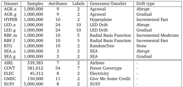
3.2.1Synthetic (top) and real-world (bottom) datasets used for
perfor-mance evaluation and comparison. . . 36
4.2.1Random numbers initialization strategy for the different activation functions . . . 45
4.2.2ELEC dataset best results obtained by RPL with different activation functions . . . 46
4.2.3COVT Evaluation . . . 47
4.2.4SUSY Evaluation . . . 48
4.2.5RPL accuracy (%) comparison against other popular data streams methods. . . 50
4.2.6SGD Batch vs Incremental . . . 50
5.2.1Map from ASCII domain to 4-symbols . . . 63
5.2.2Email address detector results . . . 63
5.2.3ESHT performance comparison against a single HT, and the best results obtained on each dataset. . . 66
5.2.4Comparing ESHT execution time against other data-streams meth-ods. . . 66
6.1.1Difference in accuracy for differenceARFsizes with respect the best one. A negative result means worse then the best. . . 71
6.1.2Average number of background learners for ARF with 100 and 50 learners. Note that RTG dataset has no drift, thus, ARF needed 0 background learners . . . 72
6.3.1Synthetic (top) and real-world (bottom) datasets used for perfor-mance evaluation and comparison. Synthetic datasets drift type: A (abrupt), G (gradual) I.F (incremental fast), I.M (incremental moderate), N (None) . . . 76
6.3.2Accuracy comparison between ARF100 and SRF with |F S| = 35 and|F S|= 50 . . . 78
6.3.3ESRF comparison with ARF100. Resource-constrained scenario: Tg= 0.01andTs= 0.001 . . . 83
6.3.4ESRF comparison with ARF100. Ts=Tg = 0.001 . . . 83
6.3.5ESRF resize factorr = 5comparison with ARF100. Tg = 0.01 and
Ts= 0.5 . . . 87
6.3.6ERF comparison with ARF100. Resource-constrained scenario:Tg =
0.01andTs= 0.001. . . 87
6.3.7ERF comparison with ARF100. Resource-constrained scenario:Tg =
0.1andTs= 0.1 . . . 88
7.4.1Datasets used in the experimental evaluation, including both real world and synthetic datasets . . . 96 7.4.2Platforms used in the experimental evaluation . . . 97 7.4.3Single Hoeffding Tree accuracy comparison . . . 97 7.4.4Single Hoeffding Tree throughput (instances per ms) on Intel (top)
and ARM (bottom) compared to MOA. ↓ indicates speed-down (MOA is faster) . . . 98 7.4.5Comparing LMHT parser overhead (instances per ms). Parser
in-cludes time to parse and process input data;No Parsermeans data is already parsed in memory. . . 99 7.4.6Random Forest Accuraccy . . . 100 7.4.7Random Forest throughput comparison (instances/ms) . . . 103
FIGURE Page
2.2.1Decition tree example. Square nodes represent internal test/split
nodes, circle nodes represent leaf nodes. . . 15
2.4.1Echo State Network: Echo State Layer and Single Layer Feed for-ward Network . . . 25
2.4.2Echo State Layer . . . 25
2.5.1Taxonomy for data streams methods used in this dissertation. Clas-sification methods: Hoeffding Tree[30], SAMKNN [95], SVM [24], Leveraging Bagging [13] and Adaptive Random Forest [44]. Re-gression methods: FIMT-DD [62], SVM [46], Adaptive Random Forest regression [42] . . . 27
3.1.1MOA’s workflow . . . 30
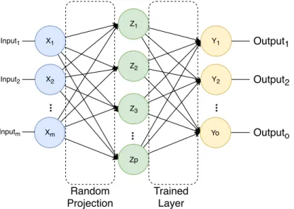
4.1.1RPL Architecture. The trained layer uses sigmoid function and MSE as the objective function, while Echo State layer (Random Projection) activation function can vary. . . 41
4.1.2Sigmoid activation function . . . 42
4.1.3ReLU activation function . . . 43
4.1.4RBF activation function using a Gaussian distance. . . 44
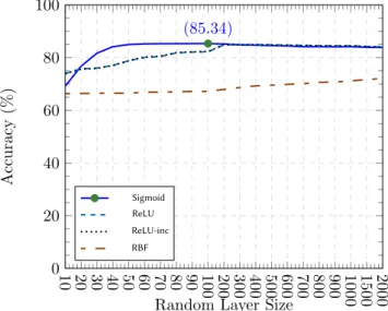
4.2.1ELEC Dataset accuracy evolution for the different random layer sizes. This plot usedµ= 0.3andη= 0.11 . . . 47
4.2.2COVT Normalized Dataset . . . 48
4.2.3SUSY Dataset . . . 49
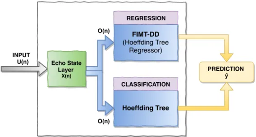
5.1.1Echo State Hoeffding Tree design for regression (top blue box) and classification (bottom blue box) . . . 54
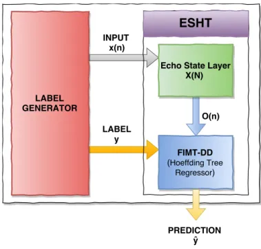
5.2.1Module internal design: label generator and ESHT . . . 55
5.2.2Countergenerator functions . . . 57
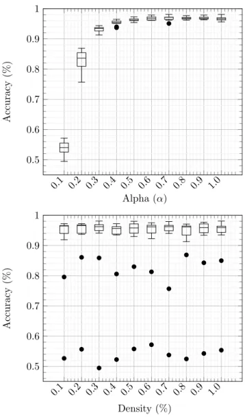
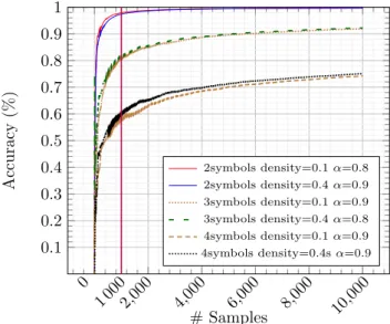
5.2.3Cumulativeloss(up) andaccuracy(bottom) on theCounterstream. 58 5.2.4Influence of parameters α and densityon the Counter stream. In each figure, the box plot shows the influence of the other parameter. 59 5.2.5lastIndexOf generation function . . . 60
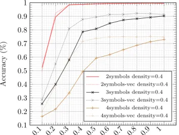
5.2.6Accuracy for thelastIndexOf function for alphabets with 2, 3 and 4
symbols. . . 60
5.2.7Encodingxsymbol as a vector . . . 61
5.2.8Effect on the accuracy of coding the input tolastIndexOf as a scalar or a vector of features (density=0.4) . . . 61
5.2.9Effect ofalphaanddensityon the accuracy forlastIndexOf . . . 62
5.2.10Cumulative loss(top) andaccuracy(bottom) evolution foremailFilter 65 5.2.11Influence of α on the ESHT accuracy; Fixed density=1.0 and 10 neurons in the ESL . . . 66
6.1.1ARF accuracy evolution with ensemble size. . . 70
6.3.1SRF accuracy evolution as the ensemble size increases . . . 77
6.3.2Influence of using a resize factor r = 1 in the accuracy distance w.r.t. ARF100 of the grow and shrink thresholds on the synthetic datasets. Negative numbers means ARF100 is better. . . 81
6.3.3Influence of using a resize factor r = 1 in the accuracy distance w.r.t. ARF100 of the grow and shrink thresholds on the real-world datasets. Negative numbers means ARF100 is better. . . 82
6.3.4Influence of using a resize factor r = 5 in the accuracy distance w.r.t. ARF100 of the grow and shrink thresholds on the synthetic datasets. Negative numbers means ARF100 is better. . . 85
6.3.5Influence of using a resize factor r = 5 in the accuracy distance w.r.t. ARF100 of the grow and shrink thresholds on the real-world datasets. Negative numbers means ARF100 is better. . . 86
7.1.1Splitting a binary tree into smaller binary trees that fit in cache lines 90 7.1.2Sub-tree L1 cache line layout . . . 91
7.1.3L1 cache line tree encoding . . . 91
7.2.1Multithreaded ensemble design . . . 93
7.2.2Instance buffer design . . . 94
7.4.1LMHT and StreamDM speedup over MOA using a single HT (Intel i7). Down bars mean speed-down (slower than MOA) . . . 100
7.4.2LMHT, StreamDM and MOA single HT throughput comparison (in-stances/ms) . . . 101
7.4.3Random Forest learning curve: COVT (top) and ELEC (bottom) . . 102
7.4.4Random Forest relative speedup on Intel i7 . . . 104
7.4.5Random Forest relative speedup on Jetson TX1 . . . 105
7.4.6Random Forest speedup on X-Gene2 . . . 105
7.4.7Intel Xeon Platinum 8160 scalability, with the parser thread stream-ing from storage (top) and memory (bottom). . . 106
1
Introduction
Machine learning (ML) is an important branch of Artificial Intelligence (AI) that focuses on building and designing algorithms to make decisions or pre-dictions about present or future events, based on learning from past events. These algorithms extract patterns and structures from examples of data in or-der to learn specific tasks without any human interaction or programming. The success of this learning process is heavily influenced by the amount, scope, and quality of input data.
Nowadays, a wide spectrum of technical and scientific areas use ML as part of its core development strategies: healthcare, manufacturing, travel, financial services, dynamic pricing, autonomous vehicles, fraud detection, fast adaptation to new user behavior, among many others. Its broad adoption in the industry is sparking new research opportunities, making ML one of the most active and prolific fields in computer science research today.
1.1
Supervised Machine Learning
This dissertation is focused on Supervised Machine Learning, a machine learn-ing task that based on trainlearn-ing dataset, builds a model capable of maklearn-ing predictions of new un-seen instances. The training dataset contains a set of labeled instances representing the specific task to learn. An instance is defined
by the values of attributes (or features) that describe essential characteristics of the task. For example, a labeled instance can be a raw image, labeled with ayesif the image contains a cat, or anootherwise.
The primary goal of a supervised algorithm is to infer a function that gen-eralizes the task to learn. This supervised algorithm processes the training dataset in order to refine the inferred function, also called model. At the out-put level, a function quantifies the current model performance by examining the model’s output for an instance (predicted label) and its correct answer (target label), and updates the model accordingly. This step is known as the induction process. A model produced by an inducer algorithm is called regres-sor if the output label belongs to the real-valued domain. When the output is a set of pre-defined (discretized) values, the model is called a classifier. Tra-ditionally, an inducer algorithm builds the model by iterating over the dataset several times until the desired error is achieved, or after a maximum number of iterations. In this dissertation, we refer to this learning strategy asbatch learningoroffline learning.
Batch learning is a challenging process that can last for hours, days or weeks, depending on the dataset. During the learning process, algorithms typically need to deal with the following challenges: noise in data, unbal-anced classes, or instances with missing values for some of the features among others. In the case of Big Data, when the dataset does not fit in memory, out-of-core or distributed learning is required, potentially affecting the final model accuracy.
In addition, offline learning works well for static problems that do not change over time. However, data generated by many of today’s application can change as time passes presenting non-stationary distributions, a fact that most batch learners do not consider. For example, TCP/IP packet monitoring [21] or credit card fraud detection [98], are situations that requires fast adap-tation and reaction to attackers’ new techniques in order to keep them away. The usual approach in these situations is to process data on–the–fly in real time.
1.2
Processing Data Streams in Real Time
Recent advances in both hardware and software fuelled ubiquitous sources generating Big Data streams in a distributed way (Volume), at high speed (Ve-locity) with new data rapidly superseding old data (Volatility). For example, the Internet of Things (IoT) is the largest network of sensors and actuators connected by networks to computing systems. This includes sensors across a huge range of settings, for industrial process control, finance, health analyt-ics, home automation, and autonomous cars, and often interconnected across domains, monitoring and functioning in people, objects and machines in real time. In these situations, storing data that is generated at an increasing
vol-ume and velocity for processing it offline can quickly become a bottleneck as time passes. Also, the uncertainty of when data will be superseded increases considerably the complexity of managing the stored data: once data is super-seded a new model is required, and methods need to discriminate at which point data became irrelevant so it should not be used for building the new model. Thus, processing this type of data requires a different approach than the traditional batch learning setup: data should be processed as a continuous stream in real time.
Extracting knowledge from data streams in real time requires fast incre-mental algorithms that are able to deal with potentially infinite streams. In addition to the challenges already present in batch learning (see Section 1.1) processing data streams in real time imposes the following challenges:
• Deal with potentially infinite data streams: data is not stored, and used exactly once (no iteration over the dataset).
• Models must be ready to predict at any moment.
• Use limited resources (CPU time and memory) with a response time in the range of few seconds (high latency) or few milliseconds (low latency).
• Algorithms should be adaptive to the evolution of data distributions over time, since changes in them, can cause predictions to become less accu-rate with time (Concept Drift).
The preferred choice for processing data streams in a variety of applica-tions is the use of incremental algorithms that can incorporate new informa-tion to the model without rebuilding it. In particular, incremental decision trees and their ensemble combinations are the preferred choices when pro-cessing Big Data streams, and are the focus of this dissertation.
1.3
Decision Trees and Ensembles for Mining Big
Data Streams
In this dissertation, we focus on the usage of the Hoeffding Tree (HT) [30], an incremental decision tree that is able to learn very efficiently and with high accuracy from data streams. Usually, single learners such as the HT are combined in ensemble methods to improve their prediction performance.
The HT is considered the state-of-the-art single classifier for processing data streams. It is based on the idea that only examining a small subset of the data is enough for deciding how to grow the model. Deciding the exact size of each subset is a difficult task, which is tackled in the HT by using the Hoeffding probability bound. The main advantage of the HT is that with high probability
the model produced will be similar to the one produced by an equivalent batch inducer. In this dissertation, we also use the Fast Incremental Model Trees with Drift Detection (FIMT-DD) [62], an incremental regressor tree that is also based on the Hoeffding probability bound. Both HT and FIMT-DD are further described in chapter 2.
Ensemble learners are the preferred method for processing data streams due to their better predictive performance over single models. Ensemble methods build a set of base models which are used in combination for obtain-ing the final label. Models built by an ensemble can use the same induction algorithm for building all models or use different inductors. In this disserta-tion, we only consider ensembles of homogeneous learners, and in particular, the Leveraging Bagging (LB) [13] and the Adaptive Random Forest (ARF) [44], two very popular methods for building ensembles of HT. Again, these two ensembles are further described in detail in chapter 2.
1.4
Neural Networks
Neural Networks (NN) are very popular nowadays, due to the large number of success stories when using Deep Learning (DL) methods in both the academic and industrial world. DL methods are even outperforming humans in complex tasks such as Image recognition [50], or playing Go [101], becoming the new state-of-the-art methods in Machine Learning.
Deep Learning aims for a better data representation at multiple layers of abstraction. In each layer, the network needs to be fine tuned. In classifica-tion, a common algorithm to fine tune the network is the Stochastic Gradient Descent (SGD) which minimizes the error at the output layer using an ob-jective function, such as the mean square error. A gradient vector is used to back-propagate the error to previous layers. The gradient nature of the al-gorithm makes it suitable to be trained incrementally in batches of size one, similar to how standard incremental training is done.
Although deep NN can learn incrementally, they have so far proved to be too sensitive to their hyper-parameters and initial conditions; for this reason NN are not considered as an effectiveoff–the–shelf solution to process data streams [80]. Observe that the ideal NN for data streams should have similar characteristics to the ones already mentioned in Section 1.2:
1. Work out-of-the-box.
2. Trained incrementally visiting each example exactly once. 3. Ready to be used at any moment.
4. Fast response time in the order of few milliseconds or few seconds. 5. React to concept drifting.
Recurrent Neural Networks (RNN) are a type of NN with an internal mem-ory that allow them to capture temporal dependencies. Training a RNN is challenging and requires a large amount of time, making them not viable for real-time learning [113, 81]. In recent years, Reservoir Computing (RC) has emerged as an alternative to RNN, aiming for a simpler and faster training [78, 64]. Reservoir Computing can be seen as an standard NN that learns from what is called a ”reservoir” unit, which is responsible for capturing the temporal dependencies of the input data stream. Although conceptually sim-pler than most RNN, computationally cheap, and easier to implement, RC still have high sensitivity to hyper-parameter configurations (i.e. small changes to any of them affect the accuracy in a non-predictable way [75]).
1.5
Contributions of this Thesis
The main goals of this thesis are to improve the Hoeffding Tree and its ensem-ble combinations from both algorithmic and implementation point of view, in order to be able to provide higher throughput and to reduce the consumption of resources while providing similar or better accuracy.
1.5.1 Neural Networks and data streams
The first contribution of this dissertation is to study the use of Neural Networks (NN) as an alternative method for processing data streams. How to use them to process data streams is not straightforward due to: 1) the fact that the NN convergence is slow, requiring large amounts of data; and 2) NN are highly sensitive to hyper-parameter configurations such as the depth or the number of neurons, which complicates their deployment in production environments. In this first contribution, we propose the use of random features in the form of a random projection layer in order to mitigate NN deployment and latency issues. We test the proposal on top of a single layer feed-forward NN, trained with SGD.
We show that NN can achieve good results on data streams classification problems; however they still require some more work to become a feasible method for processing data in real time. We also show that the HT is an easy-to-deploy method, for fast and accurate learning from data streams.
1.5.2 Echo State Hoeffding Tree learning
In this second contribution, we extend two popular incremental tree-based models for data streams, the Hoeffding Tree (HT) and the Fast Incremental Model Trees with Drift Detection (FIMT-DD), in order to capture temporal behaviour. We reuse some of the insights obtained from the first contribution in this dissertation, and propose the use of a reservoir memory that makes use of random features as a recurrent layer that enables capturing temporal
patterns. The reservoir’s output is then used as the input to a HT or a FIMT-DD. We call this combination Echo State Hoeffding Tree (ESHT).
The ESHT regression capabilities are tested on learning some typical string-based functions with strong temporal dependences. We show how the new architecture is able to incrementally learn these functions in real time with fast adaptation to unknown sequences, and we analyse the influence of the reduced number of hyper-parameters in the behaviour of the proposed solu-tion.
On classification problems, we tested our proposed architecture to learn three well-known data streams datasets. We show that our architecture can in fact improve a single HT. However, our design requires tuning of additional hyper-parameters which makes the proposal not very suitable for production environments, as opposed to other well established methods based on the use of ensembles, such as the Adaptive Random Forest (ARF).
1.5.3 Resource-aware Elastic Swap Random Forest
In this third contribution, we present an extension to ARF for processing evolv-ing data streams: Elastic Swap Random Forest (ESRF). ESRF aims at reducevolv-ing the number of trees required by the state-of-the-art ARF ensemble while pro-viding similar accuracy. ESRF extends ARF with two orthogonal components: 1) a swap component that splits learners into two sets based on their accuracy (only classifiers with the highest accuracy are used to make predictions; the rest are trained as candidates and may be swapped with the others if their accuracy is higher); and 2) an elastic component for dynamically increasing or decreasing the number of classifiers in the ensemble.
The experimental evaluation of ESRF and its comparison with the original ARF shows how these two new components effectively contribute to reduce the number of classifiers up to one third while providing almost the same accuracy. This reduction results in speed-ups, in terms of per-sample execu-tion time, close to 3x. In addiexecu-tion, we perform a sensitivity analysis of the two thresholds determining the elastic nature of the ensemble, establishing a trade–off in terms of resources (memory and computational requirements) and accuracy (which in all cases is comparable to the accuracy achieved by ARF using a fix number of 100 trees).
1.5.4 Ultra-low latency Random Forest
This final contribution presents a high-performance, scalable architecture for designing decision trees and ensemble combinations to tackle today’s applica-tion domains. The proposed architecture offers ultra-low latency (few mi-croseconds) and good scalability with the number of cores on commodity hardware when compared to other state-of-the-art implementations.
The evaluations show that on an Intel i7-based system, processing a single decision tree is 6x faster than MOA (Java), and 7x faster than StreamDM (C++), two well-known reference implementations. On the same system, the use of six cores (and 12 hardware threads) available allow processing an ensemble of 100 learners 85x faster that MOA while providing the same accuracy.
Furthermore, the proposed implementation is highly scalable: on an Intel Xeon socket with large core counts, the proposed ensemble design achieves up to 16x speed-up when employing 24 cores with respect to a single-threaded execution.
Finally, our design is highly adaptive to different hardware platforms in-cluding constrained hardware platforms such as the Raspberry Pi3, where our proposed design achieves similar performance than MOA on an Intel i7-based machine.
1.6
Organization
The rest of this dissertation is organized as follows:
Chapter 2 provides the context of the work presented in this dissertation and the fundamentals for understanding the challenges in learning from data streams. The necessary technical details are also reviewed in this chapter, alongside with a brief overview of other research works related to this disser-tation.
Chapter 3 describes the workloads used in the evaluations and provides the information on framework that has been used to evaluate the proposals in this dissertation.
Chapter 4 presents the first contribution of this dissertation, Neural net-works and data streams. This chapter details the study of neural networks as an alternative method for processing data streams in real time.
Chapter 5 details and evaluates the second contribution of this disserta-tion, theEcho State Hoeffding Tree,s an architecture for real-time classification based on the combination of a Reservoir and a HT decision tree.
Chapter 6 discusses the Resource-Aware Elastic Swap Random Forest con-tribution. We propose and evaluate two methods for reducing the resources needed on ensemble learning: Swap Random Forest (SRF) and Elastic Swap Random Forest (ESRF).
Chapter 7 discusses and evaluates the last contribution of this dissertation:
Ultra-low latency Random Forest, a high-performance scalable design for deci-sion trees and ensemble combinations that make use of the vector SIMD and multicore capabilities available in modern processors to provide the required throughput and accuracy (in the order of microseconds).
Finally, chapter 8 concludes this dissertation, summarizing its key contri-butions and results. Also, it presents potential future work and open research
lines.
1.7
Publications
The following publications contain the contributions in this dissertation as presented in journals and conferences.
Journal Publications
• Data Stream Classification Using Random Feature Functions and
Novel Method Combinations
Journal of Systems and Software, 2016
Diego Marr´on, Jesse Read, Albert Bifet, Nacho Navarro
Conference Publications
• Echo State Hoeffding Tree Learning
The 8th Asian Conference on Machine Learning, 2016, Hamilton, New Zeland
Diego Marr´on, Jesse Read, Albert Bifet, Talel Abdessalem, Eduard Ayguad´e,
Jos´e R. Herrero
• Low-latency Multi-threaded Ensemble Learning for Dynamic Big Data
Streams
IEEE International Conference on Big Data 2017, Boston, MA, USA
Diego Marr´on, Eduard Ayguad´e, Jos´e R. Herrero, Jesse Read, Albert
Bifet
• Elastic Swap Random Forest(Submitted)
International Joint Conference on Artificial Intelligence (IJCAI) 2019, China
Diego Marr´on, Eduard Ayguad´e, Jos´e R. Herrero, Jesse Read, Albert
Bifet
Poster Session
• Random Projection Layer for Neural Networks
PhD Poster Session at The Fourteenth International Symposium on In-telligent Data Analysis, 2015
Video Contest
• Random Projection Layer for Neural Networks
The Fourteenth International Symposium on Intelligent Data Analysis, 2015
https://www.youtube.com/watch?v=ySoaG-rqbr0 Diego Marr´on, Jesse Read, Albert Bifet, Nacho Navarro
2
Preliminaries and Related
Work
Learning from data streams can be considered as an infinite dynamic process that encapsulates on a single cycle, the collection of the data, the learning pro-cess, and the validation of the learned model. It mainly differs from the tradi-tional supervised machine learning by the fact that instances are not available as a large static dataset. Instead, instances are provided one by one from a continuous data stream that can last potentially forever.
Extracting useful knowledge from a potentially infinite amount of data im-poses serious challenges. First, given the vast amount of data arriving, storing it before the processing step is not feasible. Second, when collecting data for long enough periods the relations or patterns learned from data are likely to change as time passes, making old instances to become irrelevant for the current learned model. For example, trends in social networks continuously change due to different reasons. And third, data streams algorithms require sophisticated mechanisms for dealing with noise and contradictory informa-tion as they arrive, which adds another dimension to the already complicated task of providing theoretical guarantees on the performance of online learning algorithms.
The stream data mining community has approached the problem from a more practical perspective: algorithms must be designed to satisfy a list of requirements in order to efficiently process data streams. In [58, 14], authors
identified the ideal features a data stream algorithm should possess: 1. Should make a single-pass over the data.
2. The model should incrementally incorporate new information without rebuilding the entire model.
3. High speed of convergence.
4. Time for processing each instance is limited.
5. Ideally, CPU and memory consumption must be constant and indepen-dent of the number of samples processed.
6. Should react/adapt to changes while they are occurring.
Features 1-5 can in fact be met by variety of learning schemes, including batch learners where batches are constantly gathered over time, and newer models replace older ones as memory fills up [92, 20, 34, 89]. Nevertheless, incremental methods remain strongly preferred in the data streams literature [9, 11, 74] since they usually produce better results [93]. Among them, incre-mental decision trees are one of the well established methods for processing data streams, being the building block for more powerful methods such as ensemble combinations. Decision trees and their ensemble combinations are the focus of this dissertation. Another popular choice is thek-nearest neigh-bors (kNN) [100, 5, 73, 65] method, which uses the distance as the metric to find the k-nearest neighbors from the training dataset to a target data point. The original method internally stores instances in order to find the closest neighbors of each input instance which is not feasible in a real time streams setup. Extensions to the originalkNN have been proposed for dealing with the inherent performance limitations over a potentially infinite stream [66, 116, 72, 103].
Last feature, feature 6, refers to a change in the function generating the stream. When a persistent change occurs, old instances may become irrele-vant or even harmful to the current learned model, degrading its performance or invalidating it. This change is referred to as concept drifting, and data streams which present concept drift are conventionally known as evolving data streams.
This chapter is organized as follows. In Section 2.1, we give the necessary background for understanding concept drifting and the challenges it presents in a data streams setup. Incremental decision and regression trees are intro-duced in Section 2.2, giving details about the Hoeffding Tree and FIMT-DD, the two methods used in the contributions of this dissertation. Section 2.3 in-troduces ensemble learning, and give relevant details for the ensemble meth-ods that are also used in this dissertation. Finally, Section 2.4 reviews the current status of Neural Networks applied to data streams, as an alternative methodology to decision trees and ensemble methods.
2.1
Concept Drifting
Learning from data streams is challenging since conventional machine learn-ing methods assume that the data is static (i.e., the data distribution is sta-tionary), while many situations in the real world tend to be dynamic (i.e., non-stationary data distribution). For example, trending topics in social networks or people’s opinion about a celebrity/politician change frequently, frauds evolve constantly. These situations imply a change in the target con-cept (e.g., what was interesting in the past it is not interesting anymore) po-tentially invalidating old patterns previously learned before the change. This highlights another important aspect when processing data streams: the strong temporal dependence of data, in the sense that only recent data is relevant for the current concept.
A concept drift is a persistent change in the underlying probability distri-bution generating the data stream, and it should not be confused with outliers (which are transient). Different reasons can cause a change in the concept; however, in practice, the focus of attention is the speed of the change. De-pending on that, drifts can be of any of the following types [112]:
• Abrupt/Sudden: the concept (data distribution) changes abruptly from
one time instance (t) and the next one (t+ 1). All instances∈[0, t]are generated using conceptC1, and starting fromt+ 1samples are drawn from conceptC2.
• Gradual: the change to the new concept takes a while to complete.
While the change is active, the probability of seing samples from C2 increases while the probability of seing samples fromC1decreases. This transition is usually monotonic, but not necessarily.
• Incremental: change also takes a while to complete, but unlike in
grad-ual drifts, concepts are blended while drift is active. This type of drift is difficult to detect since it can be easily confused with a series of short abrupt drifts. If this drift is active during a short period of time, it is called incremental fast drift; otherwise, it is known as an incremental moderate.
• Recurrent: When a previous concept re-appears over time. Note that a
previous concept can re-appear suddenly, incrementally or gradually. The presence of a concept drifting is usually reflected in the model perfor-mance: the number of errors gradually or abruptly increase due to the incon-sistency between the induced model and newly arriving instances. Therefore, to ensure a proper model adaptation to the current concept, appropriate mon-itoring of the learning process is necessary.
There are several strategies for dealing with concept drifting [112, 37]. In this dissertation, we use the ADWIN [10] drift detector which provides theoretical guarantees about false positives and negatives.
2.1.1 ADWIN Drift Detector
The Adaptive Windowing (ADWIN) [10] is a concept drift detector that uses an adaptive size sliding window algorithm for detecting changes in data streams. Its main features are: 1) the sliding window is automatically resized depending on the stream characteristic, 2) it provides theoretical guarantees on the ratio of false positives and false negatives when detecting drifts, and 3) it makes no assumptions about the data.
The ADWIN algorithm keeps a sliding windowW, with the lastnrecently received values. Input values can be a binary stream representing errors in classification or a stream of real values representing the loss. The algorithm repeatedly split W into two sub-windows w0 and w1 at different points in the windowW. For each split point, it computesµˆw0 andµˆw1 corresponding to the average of the values in sub-windows w0 and w1, respectively. If the difference in the averages is above a thresholdcut (i.e.,| µˆw0 - µˆw1 |> cut) this indicates a significant drop in performance caused by a change in the error distribution, and a change in the stream is signaled. When a drift is detected, older elements in W are dropped until | µˆw0 - µˆw1 | is below the threshold
cut; this causesW to shrink.
The thresholdcut is computed as shown in equation 2.1, whereW is the
current length of W, andm is the harmonic mean of the two sub-windows averages µˆw0 and µˆw1 (as shown in equation 2.2). Observe that the only parameter required to configure the ADWIN is δ ∈ (0,1) representing the confidence in applying the cut-offcut.
(2.1) cut = r 1 2mln 4W δ (2.2) m= 1 1 ˆ µw1 + 1 ˆ µw1
ADWIN does not explicitly store all elements inW. Instead, it compresses values using a variation of the exponential histogram [26] requiring only O(logW) memory for storing values, whereW is the length of the window. This way, instead of testing W split points for dividing W into w0 and w1, ADWIN only needs to test O(logW) split points.
2.2
Incremental Decision and Regression Trees
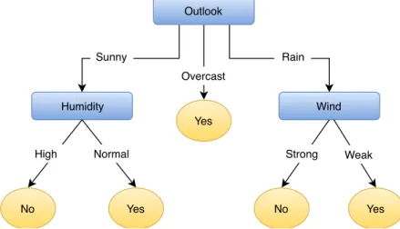
Decision and regression trees use tree-based data structures for modelling complex decision making. They consist of nodes, branches and leaves as shown in Figure 2.2.1. Each internal node (blue squares) tests on a sin-gle attribute (e.g., outlook attribute) in order to chose the appropriate path. Branches are the paths connecting two nodes from two subsequent levels in the tree structure; a node has as many branches as values it can take. Leaf nodes (yellow circles) is where the actual label prediction is done; however, they also contain the necessary information for choosing the next split at-tribute when necessary. In that case, the leaf node is substituted by an internal node representing the attribute to test on.
Figure 2.2.1: Decition tree example. Square nodes represent internal test/s-plit nodes, circle nodes represent leaf nodes.
Outlook Humidity Wind Yes No Yes No Yes Sunny Overcast Rain Normal
High Strong Weak
Decision trees are built using a divide-and-conquer strategy for partition-ing the data into smaller subsets. This partitionpartition-ing works at attribute (or feature) space, which is recursively partitioned into smaller subsets until a stopping criterion is met. For example, in Figure Figure 2.2.1, the Humid-ity represents the data partition using all instances that hasOutlook=Sunny, and similarly on the rest of nodes. How an attribute is selected for splitting the attribute space is algorithm-dependent, but in general, it is an expensive operation in term of memory and CPU time.
Incremental tree-based models have been proposed in the literature for classification [108, 109] and for regression [110]. Among incremental mod-els, the Hoeffding Tree (HT) [30] is considered the state-of-the-art single clas-sifier for data streams classification, being widely used in this dissertation. In Chapter 5, we also use the FIMT-DD [62], an incremental regressor tree based on the same principles than the HT. Both are further detailed in the next two
subsections.
2.2.1 Hoeffding Tree
The Hoeffding Tree (HT) [30] is an incrementally induced decision tree, and it is considered the state-of-the-art learner for data streams classification. It provides theoretical guarantees that the induced tree is asymptotically close to a tree that would be produced by a batch learner when the number of instances is large enough.
The induction of the HT mainly differs from the induction of batch decision trees in that it processes each instance only once, at the time of arrival (instead of iterating over the entire dataset). Instead of considering the entire training data for choosing the best attribute to split on, the HT states that it may be sufficient only to consider a small subset of the data seen at a leaf node. The Hoeffding Bound (HB) [54] is used to decide the minimum number of instances required with theoretical guarantees. It states that the deviation of an arbitrarily chosen hypotheses with respect the best one is no higher thanwith probability 1−δ (whereδ is the confidence level). The very nice property of this test is that it works independently of the data distribution, at expenses of requiring more instances to reach the same level of error than the equivalent distribution-specific tests.
Algorithm 1 shows the HT induction algorithm. The starting point is an HT with a single node (the root). Then, for each arriving instanceXthe induction algorithm is invoked, which routes through HT the instanceX to leafl (line 1). For each attributeXiin X with valuejand labelk, the algorithm updates
the statistics in leaf l (line 2) and the number of instances nl seen at leaf l
(line 3).
Splitting a leaf is considered every certain number of instances (grace pa-rameter in line 4, since it is unlikely that an split is needed for every new instance) and only if the instances observed at that leaf belong to different labels (line 4). In order to make the decision on which attribute to split, the algorithm evaluates the split criterion functionGfor each attribute (line 5). Usually this function is based on the computation of the Information Gain, which is defined as:
(2.3) G(Xi) = L X j Vi X k aijk Tij log(aijk Tij ) ∀i∈N
beingN the number of attributes,Lthe number of labels and Vi the number
of different values that attributeican take. In this expressionTij is the total
number of values observed for attributeiwith labelj, andaijk is the number
of observed values for which attributeiwith labeljhas valuek. The Informa-tion Gain is based on the computaInforma-tion of theentropywhich is the sum of the
probabilities of each label times the logarithmic probability of that same la-bel. All the information required to compute the Information Gain is obtained from the counters at the HT leaves.
The algorithm computes G for each attribute Xi in leaf l independently
and chooses the two best attributes Xa and Xb (lines 6–7). The Hoeffding
Bound is used for testing the hypotheses thatG(Xa)andG(Xb)deviate from
each other. Therefore, an split on attribute Xa occurs only ifXa andXb are
not equal, andG(Xa)−G(Xb)> , whereis the Hoeffding bound which is
computed (line 8) as:
(2.4) =
s
R2ln(1
δ)
2nl
being R = log(L) and δ the confidence thatXa is the best attribute to split
with probability 1−δ. Since the value of decays monotonically with the number of instances seen, a leaf node only needs to accumulate examples untilbecomes smaller thanG(Xa)−G(Xb)for choosing Xaas the splitting
attribute. If the two best attributes are very similar (i.e. Xa−Xb tends to0)
then the algorithm uses a tie threshold (τ) to decide splitting (line 9).
Once splitting is decided, the leaf is converted to an internal node testing on Xa and a new leaf is created for each possible value Xa can take; each
leaf is initialised using the class distribution observed at attributeXacounters
(lines 11–13).
Leaf Classifiers
Although it is not part of the induction algorithm shown in Algorithm 1, pre-dictions are made at the leaves using leaf classifiers built using the statistics collected in them. Each classifier is trained using only the instances seen at its leaf node, and usually, reuses the same statistics collected for deciding the split attribute.
The Majority Class Classifier (MCC) is the simplest classifier used in the HT, which simply tags the arriving instance with the most frequent label seen in that leaf. It requires no extra statistics other than those already being col-lected at leaf nodes, and its computational cost is almost negligible.
Another very common classifier is Naive Bayes (NB) [38]. It is a relatively simple method that can reuse the statistics already collected at each leaf node. An advantage of this classifier is that it only requires a small number of train-ing data to estimate the parameters necessary for classification. By maktrain-ing the naiveassumption that all attributes are independent, the joint probabili-ties can be expressed as shown in Equation 2.5.
(2.5) p(Ck|x) =p(Ck) n
Y
i=1
Algorithm 1Hoeffding Tree Induction
Require:
X: labeled training instance DT: current decision tree
G(.): splitting criterion function
τ: tie threshold
grace:splitting-check frequency (defaults to 200)
:Hoeffding Bound
1: Sort X to a leaflusing HT
2: Update attribute counters inlbased on X
3: Update number of instancesnlseen atl
4: if(nl mod grace=0) and (instances seen at lbelong to more than 1
dif-ferent classes)then
5: For each attributeXiinlcomputeG(Xi) 6: LetXabe the attribute with highestGinl
7: LetXb be the attribute with second highestGinl 8: Compute Hoeffding Bound
9: ifXa6=XbandGl(Xa)−Gl(Xb)> or < τ then 10: Replacelwith an internal node testing onXa 11: foreach possible value ofXado
12: Add new leaf with derived statistics fromXa
13: end for
14: end if
15: end if
It is not not clear which classifier among MCC or NB is the best option. In some situations, NB can initially outperform the MCC, but, as time passes NB can be eventually overtaken by MCC. To address this situation, the Adaptive Naive Bayes HT was proposed [55] which only uses NB classifier when it outperforms MC.
Hoeffding Tree and Concept Drift
Concept drift detection and adaptation requires the use of extra modules (drift detectors), which are not included in the original HT algorithm presented in [30]. HT can adapt to a concept drift by either adapting the tree structure, or by starting a new empty tree.
Adapting the tree structure is done by identifying which sub-tree is af-fected by the drift. Since a drift in an attribute may invalidate its entire sub-tree, per-attributes drift detectors are used for determining the drifting attribute (the root node of the affected sub-tree). A common approach in data streams is the use of option trees where a new candidate sub-tree is started on the drifting attribute. Both candidate and original sub-trees are
trained in parallel until enough evidence is collected for dropping one of then by either confirming the drifting or a false positive. Extensions to the original HT have been proposed using this strategy, such as the Concept-adapting Very Fast Decision Trees CVFDT [59] and the Hoeffding Adaptive Tree (HAT) [11]. Dropping a tree and starting a new empty tree seems to be the simplest strategy: when a drift is detected the entire tree is substituted by a new empty one. This strategy only requires one drift detector monitoring the overall tree performance, which consumes considerably less memory and CPU-time. The drawback is that the there is a lag in time while the tree achieves good performance again. Ensemble combinations used in this dissertation prefer this strategy (as shown in the next section) due to its simplicity and the fact that in ensembles this drawback can be hidden by the rest of the trees.
2.2.2 FIMT-DD
The Fast Incremental Model Trees with Drift Detection (FIMT-DD)[62] is an incrementally induced regression tree which is also based on use of the Ho-effding Bound for growing the tree structure. In the FIMT-DD, the tree struc-ture is a binary tree, i.e. each internal node has two branches.
FIMT-DD uses the same induction strategy as in the HT with proper adap-tations for regression, as shown in Algorithm 2. The major difference with respect the HT is that the FIMT-DD incorporates a mechanism for adapting the tree structure in the presence of a concept drift is detected (lines 4–6). The other differences are the necessary changes for enabling the induction process to work in regression problems: 1) how leaf nodes select next attribute to split on (lines 10–14); and 2) predictions are made using a regressor instead of a classifier (not shown in Algorithm 2).
The algorithm computes Standard Deviation Reduction for each attribute in a leaf mode. LetAbe the attribute with highest SDR, andBthe second one. The ratiorbetweenSDRAandSDRBis computed as shown in equation 2.6.
The attribute is chosen as for splitting ifr > , whereis the Hoeffding bound already seen in equation 2.4.
(2.6) r = SDRB
SDRA
Prediction at leaf nodes is done using a perceptron with linear output. For each arriving instance an incremental Stochastic Gradient Descent is used for training the perceptron, using all numeric attributes (including those used during the tree traversal).
As mentioned above, in the presence of a concept drift the FIMT-DD starts a new sub-tree for the region where drift is detected (line 5). Both, new and old, sub-trees are grown in parallel until one of them is discarded. The drift detector used in FIMT-DD is the Page-Hinckley [85].
Algorithm 2FIMT-DD Induction
Require:
X: labeled training instance DT: current decision tree structure
G(.): splitting criterion function
grace:splitting-check frequency (defaults to 200)
:Hoeffding Bound
1: foreach example in the streamdo 2: Sort X to a leaflusing DT
3: Update change detection tests on the path
4: ifChange is detectedthen 5: Adapt the model tree
6: else
7: Update statistic inlbased on X
8: Update number of instancesnlseen atl 9: if(nl modgrace=0)then
10: Find two best split attributes (XaandXb) 11: ifGl(Xa)−Gl(Xb)> then
12: Replacelwith an internal node testing onXa 13: Make two new branches leading to empty leaves
14: end if
15: end if
16: end if
17: end for
2.2.3 Performance Extensions
The unfeasibility to store potentially infinite data streams has led to the pro-posal of classifiers able to adapt to concept drifting only with a single pass through the data. Although the throughput of these proposals is clearly lim-ited by the processing capacity of a single core, little work has been conducted to scale current data streams classification methods.
For example Vertical Hoeffding Trees (VHDT [69]) parallelize the induc-tion of a single HT by partiinduc-tioning the attributes in the input stream instances over a number of processors, being its scalability limited by the number of attributes. A new algorithm for building decision trees is presented in SPDT [6] based on Parallel binning instead of the Hoeffding Bound used by HTs. [104] propose MC-NN, based on the combination of Micro Clusters (MC) and nearest neighbour (NN), with less scalability than the design proposed in this paper.
Related to the parallelization of ensembles for real-time classification, [79] has been the only work proposing the porting of the entire Random Forest algorithm to the GPU, although limited to binary attributes.
2.3
Ensemble Learning
Instead of focusing on building the most accurate model, ensemble methods [22, 111, 68] combine a set of weak models (base models) for achieving bet-ter predictive performance than single models [36, 29]. The main belief in literature is that combining weak models allow wider exploration of different representations or search strategies if there is enough diversity among base learners [88, 94, 83, 84, 49]. Although there is no accepted definition for diversity, the consensus is that ensembles should ”spread” the error equally among all learners in the ensemble, so incorrect predictions can be corrected by the majority of the learners in the combination step [70].
Diversity in data streams is usually achieved by introducing a random com-ponent during the building of the model, since exhaustive exploration of all possible combinations can quickly become a heavy or an impossible task. Ran-domization in ensembles can be at different levels:
• Input: by creating random subsets from the input data. A well-known al-gorithm for manipulating the input is the Bagging alal-gorithm [17], which creates a different sub-set for each learner by sampling from the original dataset allowing repetitions
• Learner: randomness is introduced in order to improve the exploration of different strategies (sub-sets in this case). For example, Random Forests (RF) [18] use a variation of decision trees that only considers a random subset of the features in the leaf nodes.
The other important ensemble component, as mentioned in [88], is learner’s output combination to form the final prediction. A detailed study of different combination methods is presented in [107]. The implicit voting schemes used in the methods we use are the Majority Vote (MV), and the Weighted Majority Vote (WMV) scheme which are very similar: both schemes combine outputs using a fixed simple function (such as aggregation), and then the most voted label is select as the final prediction. The only difference is that MV assume all learners are equally important, while in WMV, a weight decides each learner importance when combining the outputs.
The way predictions can be combined is a direct consequence of how learn-ers interact with each other. According to [43], ensembles can be categorized in the following types depending on their architecture:
• Flat: Learners are trained independently on the input data, then their predictions are combined using a simple function (voting scheme). This architecture is the most common architecture used by ensemble meth-ods. Examples of ensembles using this architecture are Online Bagging [86], Leveraging Bagging [13] and Adaptive Random Forest [44].
• Meta-Learner: In this category, a meta-dataset substitutes the original input data, and it is used for training meta-learners. The meta-dataset can be created from the output of other learners, such as in Restricted Hoeffding Tree [9], or from data describing the learning problem.
• Hierarchical: Members are combined in a tree-like structure, including
the cascading or daisy chain. The most notable method for data streams in this category is the HSMiner [16], which breaks the classification problem into tiers in order to prune irrelevant features.
• Network: The ensemble is viewed as a graph, which vertices represent
learners and the edged represent how learners are connected according to a specific criterion. New connections and vertices can be added at any moment, resembling more to a computer network than to a static graph. For example, SFNC [4] uses a Scale-Free Network model to generate the connections (edges).
The focus of this thesis is in flat ensemble methods, due to their simpler architecture, and the fact that they usually make fewer assumptions about the data distribution. The specific methods used in this dissertation are Leverag-ing BaggLeverag-ing (LB) and the Adaptive Random Forest (ARF), which are described in the following subsections. Previous to describing LB and ARF, we describe the Online Bagging (OB) method since it is the base for both LB and ARF.
2.3.1 Online Bagging
The Online Bagging (OB) [86] is a flat ensemble method that enforces diver-sity by introducing randomization at input data, and uses the majority voting scheme for combining learners predictions. OB is the streaming adaptation of the well-known Bagging method introduced in [17].
In the original algorithm, each learner in the ensemble is trained using a subset of the original dataset which is created using the so-called sampling with repetition, i.e., each instance from the original dataset can appear 0, 1, or more in a subset. However, sampling requires storing all instances which is not feasible in the data streams setup.
The OB simulates the sampling with repetition by weighting each input instance instead of storing it. Weights are sampled from a Poisson distribution probability withλ= 1, and are expected to be0,1, or>1in frequencies 37%, 37%, 26% respectively. Observe that an instance with weightw = 0 means the instance is not present in the subset, whilew >1implies that the instance appears more than once.
2.3.2 Leveraging Bagging
Leveraging Bagging (LB) [13] is an extension of the OB ensemble method, that uses a HT as the base learner and includes a drift detection method.
This method leverages the use of the Poisson distribution by using aλ= 6, altering the output values distribution such as: 0.25% values equal to zero, 45% values lower than six, 16% of values equal to 6, and 39% values greater than 6. By using λ = 6, the ensemble is using more instances for training, which improves the learning of the ensemble.
LB is an adaptive ensemble method, i.e., it can detect and react to concept drifting. As soon as drifting is detected in any of thelearners, LB starts a new empty tree in order to replace the one with higher error. LB by design uses the ADWIN drift detector.
2.3.3 Adaptive Random Forest
The Adaptive Random Forest (ARF) [44] was introduced recently as a stream-ing adaptation of one of the most used machine learnstream-ing algorithms in the literature, the Random Forest (RF) [18]. ARF has become a popular ensemble method in data streams due to its simplicity in combining leveraging bagging with fast random Hoeffding Trees, a randomized variation of the HT that adds diversity at the learner level.
The Random Hoeffding Tree splits the input data by only considering a small subset of the attributes at each leaf node when growing the tree. When a leaf node is created, b√Nc attributes are randomly selected from the N
original attributes, and used to decide the next attribute to split on.
At input level, ARF enforces diversity by sampling with repetition using a Poisson(λ= 6), as in LB. At the output level, ARF uses the Weighted Majority Voting scheme in which each classifier is weighted using its accuracy.
To cope with evolving data streams, ARF uses a drift detection method based on a two threshold scheme: 1) a permissive threshold triggers a drift warning, which starts a local background learner; and 2) a second threshold confirms the drift, in which case the background learner substitutes the origi-nal learner. Although ARF is not tailored to any specific detector, the preferred (default) option is ADWIN.
2.4
Neural Networks for Data Streams
Most Neural Networks (NN) applications assume stationary data distribution where the training is done in a batch setup using a fixed network architecture (number of layers, neurons per layer). The training step is computationally very costly, which depending on the task to learn, it can take days or even weeks to reach the desired error level.
The Back Propagation (BP) [51, 96] algorithm is widely used for training neural networks in conjunction with the Stochastic Gradient Descent (SGD) [23, 47] for minimizing the error at the output layer. Although SGD can be trained incrementally and has strong convergence guarantees, its main issue is that its convergence is slow, which in the data stream setting contradicts
feature 4, that time for processing each instance is limited, mentioned at the beginning of this Chapter.
In the Deep Learning literature, extensions for accelerating the SGD con-vergence have been proposed, such as AdaGrad [32], RMSProp [106] and Adam [67]. AdaGrad uses a per-element (in the gradient vector) learning rate which automatically increases or decreases depending if an element is sparse or dense respectively. The learning rate is adapted based on the sum of squared gradients in each dimension. RMSProp and Adam use a moving average of the squared gradients for updating a per-element learning rate.
The depth of the network (number of layers) also influences the SGD con-vergence: shallow networks converge faster than deeper ones. In 2018, an Online Deep Learning framework was proposed [97] that dynamically increas-es/decreases the number of layers using a shallow to depth approach, using the Hedge algorithm [35] in conjunction with BP in the training process.
Recurrent Neural Networks [53, 41, 52, 28] have a natural ability for cap-turing temporal dependencies, a desirable feature for processing data streams since they typically present strong temporal dependence. At the moment of starting this dissertation the most interesting RNN for data streams was the so-called Reservoir Computing [99, 76, 77], and in particular the Echo State Network (ESN) [64]: a shallow RNN that aims for a simpler and faster train-ing [78, 64]. As detailed in the next subsection (2.4.1), despite ESNs betrain-ing more straightforward than other RNNs, they are computationally very cheap and very easy to implement being able to model non-linear patterns [87].
With the recent advances in Deep Learning and Neural Networks, some works have been proposed in the context of online learning and data streams, most of them after the work in this dissertation was started. Generative Adver-sarial Networks (GANs) [45] were introduced in 2014 and recently become very popular due to their ability to learn data representations and generate synthetic samples that are almost indistinguishable from the original data. In 2017 GANs were proposed in the context of online learning [7] where au-thors use GANs for storing historical training data instead of explicitly store the data, this way only the model is propagated instead of the actual data. Also, their proposed design can adapt to new classes online by resizing the output layer. However, it is not tested with concept drifting nor any typical data streams dataset. Other works include the use of forgetting mechanisms [39], or are based on Randomized Neural Networks [115] such as [90].
2.4.1 Reservoir Computing: The Echo State Network
The Echo State Network (ESN) uses aresevoirunit (Echo State Layer in Figure 2.4.1) which is responsible for capturing the temporal dependencies of the input data stream, allowing the ESN to act as dynamic short-term memory. The ESL is connected to a Single Layer Feed-Forward Network (SLFN), that
is trained using the standard Stochastic Gradient Descent (SGD) with Back Propagation.
Figure 2.4.1: Echo State Network: Echo State Layer and Single Layer Feed forward Network
Figure 2.4.2 details the ESL. It is a fixed single-layer RNN that transforms time-varying input U(n) to a spatio-temporal pattern of activations on the output O(n). The input U(n)∈RK is connected to the echo state X(n)∈
RN through a weight matrixWin
N,K. The echo state is connected to itself through
a sparse weight matrixWres
N,N.
Figure 2.4.2: Echo State Layer
Status update in the ESL involves no derivatives and no error back prop-agation typically required for training other RNNs. The update is a simple forward step combined with a vector addition, as shown in equations 2.7-2.9. The reduced number of computations needed by the update combined with the ability of modeling temporal dependencies (typically present in data streams), makes the ESL very attractive for real-time analysis.
(2.7) w˜(n) = tanh(WinU(n) +WresX(n−1))
(2.9) O(n) =X(n)
The hyper-parameterα is used during the echo stateX(n) update, and con-trols how the echo state is biased towards new states or past ones, i.e., concon-trols how sensible theX(n) is to outliers. This resembles the update formula for the momentum explained in Section 4.1.1, where defining(X) = ∇Ct−2 as the ”new concept to incorporate”, andwt=X(n)as the average, we obtain an
almost identical formula; the ESL is also behaving as an exponentially moving average.
Optionally, the input U(n) can be connected to the output O(n) ∈ RN
using a weight matrixWout
N,K. In this work, however, we do not useWN,Kout (see
Eq. 2.9) since it requires the calculation of correlation matrices or pseudo-inverses which are computationally costly.
The ESL uses random matrices (Win andWres) that, once initialized, are
kept fixed (as in the RPL in Chapter 4.1). The echo state X(n)is initialized to zero, and it is the only part that is updated during the execution. Note that the echo stateX(n)only depends on the input to change its state. As shown in equation 2.8, calculating X(n) is computationally inexpensive since it only computes a weighted vector addition; the update cost is almost negligible when compared to other RNNs training algorithms.
The ESL needs to satisfy the so-called Echo State Property (ESP): for a long enough input U(n) the echo state X(n) has to wash out any information from the initial conditions asymptotically. The ESP is usually guaranteed for any input if the spectral radius of the ESL Weight Matrix is smaller than unit but is not limited to it: under some conditions the larger the amplitude of the input the further above the unit the spectral radius may be while still obtaining the ESP [114].
Although conceptually simpler than most RNN, computationally cheap, and easier to implement, the ESN still have high sensitivity to hyper-parameter configurations (i.e., small changes to any of them affect the accuracy in a non-predictable way). In order to reduce the number of hyper-parameters, and to accelerate the convergence of the model we propose to replace the SLFN originally included in the ESN with an incremental decision tree, in particular a Hoeffding Tree.
2.5
Taxonomy
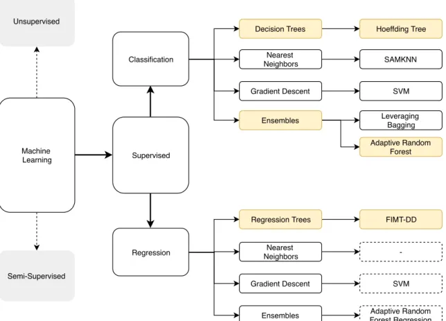
Figure 2.5.1 presents a taxonomy for the data streams methods used in this dissertation. Those methods that we specifically extend in our contributions are marked with a yellow box. Regression methods marked with a dashed box are shown for completeness (they are not used in this dissertation). To the best of our knowledge we could not find any nearest neighbor proposal
Machine Learning Unsupervised Classification Semi-Supervised Decision Trees Nearest Neighbors Gradient Descent Ensembles Regression Regression Trees Nearest Neighbors Gradient Descent Ensembles Supervised Hoeffding Tree SAMKNN SVM Leveraging Bagging FIMT-DD -SVM Adaptive Random Forest Regression Adaptive Random Forest
Figure 2.5.1: Taxonomy for data streams methods used in this dissertation. Classification methods: Hoeffding Tree[30], SAMKNN [95], SVM [24], Leve-raging Bagging [13] and Adaptive Random Forest [44]. Regression methods: FIMT-DD [62], SVM [46], Adaptive Random Forest regression [42]
for data streams regression. We also show other machine learning areas (grey boxes) for a better perspective of the scope of this dissertation.
3
Methodology
In order to evaluate some of the proposals in this dissertation, we made ex-tensive use of the MOA (Massive Online Analysis) framework [12], a software environment for implementing algorithms and running experiments for on-line learning from data streams in Java. MOA implements a large number of modern methods for classification and regression tasks, including Hoeffding Tree, K-Nearest Neighbors, Leveraging Bagging and Adaptive Random For-est, among others. Various combinations of these methods were used in the evaluations as a baseline comparison for our proposals.
This chapter also details the datasets used in the evaluations, which com-prises real-world and synthetic ones (generated using the synthetic stream generators included in MOA). For each generator, its main characteristics are further detailed in this chapter alongside with the configuration used in MOA for generating each dataset.
This chapter is organized as follows. Section 3.1 describes the MOA frame-work. Real-world and synthetic datasets used in the evaluations are described in Section 3.2. A table that summarizes all datasets (real-world and synthetic) can be found in Section 3.2.3. Finally, Section 3.3 details the metrics an