1-1-2017
Multi-Way Factorization Machine For Sentiment
Analysis
Jingwei Zhang
Wayne State University,Follow this and additional works at:http://digitalcommons.wayne.edu/oa_theses
Part of theComputer Sciences Commons
This Open Access Thesis is brought to you for free and open access by DigitalCommons@WayneState. It has been accepted for inclusion in Wayne State University Theses by an authorized administrator of DigitalCommons@WayneState.
Recommended Citation
Zhang, Jingwei, "Multi-Way Factorization Machine For Sentiment Analysis" (2017).Wayne State University Theses. 599.
by
JINGWEI ZHANG THESIS
Submitted to the Graduate School of Wayne State University,
Detroit, Michigan in partial fulllment of the requirements for the degree of
MASTER OF SCIENCE 2017
MAJOR: COMPUTER SCIENCE Approved By:
2017
me get better quality results. Without his guidance, I would not have the honor to show my research in this thesis.
Also, I would like to appreciate my parents for their seless love which support me spiritually throughout writing this thesis.
Acknowledgements iii
LIST OF TABLES vi
LIST OF FIGURES vii
CHAPTER 1: INTRODUCTION 1
1.1 Thesis objective . . . 1
1.2 Thesis motivation . . . 2
1.3 Our contribution . . . 3
1.4 Organization . . . 3
CHAPTER 2: RELATED WORKS 5 2.1 Feature representation and embedding . . . 5
2.1.1 One-hot encoding . . . 6
2.1.2 Bag of Words . . . 6
2.1.3 Continuous Bag of Words . . . 7
2.1.4 Skip-gram . . . 9
2.2 Text classication models . . . 10
2.2.1 Naïve Bayes . . . 10
2.2.2 Decision Tree and Random Forest . . . 10
2.2.3 k-Nearest-Neighbours . . . 11
2.2.4 Support Vector Machine . . . 11
2.2.5 Neural Networks . . . 13
2.3 Sentiment analysis methods . . . 16
2.3.1 Earlier research . . . 17
2.3.2 Recent research . . . 18 iv
CHAPTER 3: MULTI-WAY FM METHOD 21 3.1 Two-way FM . . . 21 3.2 Features' interaction . . . 23 3.3 Learning FM . . . 24 3.4 Multi-way FM . . . 25 3.5 Summary . . . 26 CHAPTER 4: Experiments 27 4.1 Methodology . . . 27 4.2 Datasets . . . 28
4.3 Model tunning with k . . . 28
4.4 Model tunning with m . . . 30
4.5 Method comparison . . . 30
CHAPTER 5: CONCLUSION 33 5.1 Summary of Contributions . . . 33
5.2 Future Research Directions . . . 33
REFERENCES 35
ABSTRACT 36
AUTOBIOGRAPHICAL STATEMENT 37
Table 2.2 AUC value reference Table . . . 20 Table 3.3 User movie review record Table . . . 23 Table 3.4 Properities of the Stochastic Gradient Descent (SGD) Learning Algorithm 25 Table 4.5 Performance comparison . . . 32
Figure 2.2 The structure of multi-word Continuous Bag of Words model . . . 8
Figure 2.3 The structure of Skip-gram model . . . 9
Figure 2.4 The structure of a single neural unit which includes 3inputs: x1,x2, x3, one constance, and one output: hW(x) . . . 14
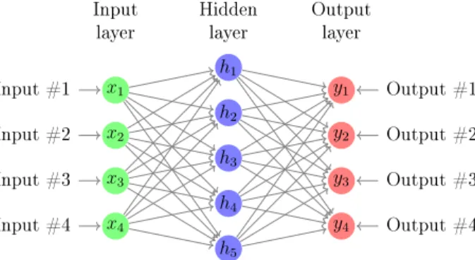
Figure 2.5 The structure of a general Neural Networks (NN) model . . . 15
Figure 4.1 The procedure of our multi-FM approach . . . 28
Figure 4.2 The length distribution of Twitter data . . . 29
Figure 4.3 The length distribution of movie review data . . . 30
Figure 4.4 The robust performance of our multi-way FM approach achieved by tun-ning a single parameter k . . . 31
Figure 4.5 The robust performance of our multi-way FM approach achieved by tun-ning a single parameter m . . . 32
CHAPTER 1: INTRODUCTION
Sentiment analysis is a process that learns the relationship between people's emotion and the corresponding text. It widely exists in lots of areas. Although it includes several tasks, such as opinion analysis, emotion mining, all of them belong to a part of sentiment analysis, which means they are now all under the tree of sentiment analysis or opinion mining. People from industry usually use single term sentiment analysis while people from academia often use sentiment analysis and opinion mining together. Actually, the meaning of them are same. They basically represent the same eld of study [8].
1.1 Thesis objective
Sentiment analysis has attracted considerable interest from both research community and industry. The purpose of sentiment analysis is to exploit classication models which can analyze sentiment information from texts in human natural language area includes opinions and emotions, with the aim to generate structured and actionable knowledge which can be applied by a decision-making system. As the fast developing of social networking, sentiment analysis has been considered as a signicant role.
Sentiment analysis is made of two successive stages, preprocessing and learning. For preprocessing, there are several popular word feature representation and embedding methods include Bag of Words (BOW), Continuous Bag of Words (CBOW), and Skip-gram (SG) [10]. All of them convert textual data into feature vectors and matrices. However, Bag of Words (BOW) simply represents words in a discrete and sparse space spanned by a word dictionary whereas Continuous Bag of Words (CBOW) and Skip-gram (SG) are feature embedding approaches that train a shallow and two-layer Neural Networks (NN) to reconstruct linguist context of words. For learning, classication methods learn the relationship between input matrices and sentiment labels.
Existing methods are eective either for longer or shorter textual data but not both. In this thesis, we propose using multi-way Factorization Machine (FM) as a new sentiment
analysis method for integrated feature embedding and sentiment classication. Importantly, our approach is suciently versatile and exible that achieves a robust performance for classifying a variety of textual documents of diverse lengths by adjusting a single tuning parameter [5].
1.2 Thesis motivation
The history of linguistics and Natural Language Processing (NLP) is not short. How-ever, there is seldom research about sentiment analysis earlier than the year 2000. After that, there is more and more research focusing on sentiment analysis. The explanations of this phenomenon are as follows: rst of all, it is widely applied in everywhere. Those industry involving sentiment analysis has taken advantages of the fast increasing commercial applications. Under this circumstance, a high motivation for research has been generated. Next, numbers of challenging research subjects have been made from it, and they have not been studied yet. Third, we hardly have large volume sentiment dataset in the area of web social media until current days. After that, basing on large volume dataset, numbers of studies and experiments can be carried out. It is no wonder that there are numbers of sentiment analysis research concentrate on social media data. Moreover, social media data is widely studied in sentiment analysis right now. Therefore, the deep impact of sentiment analysis will not only make contributions to NLP but also will make contributions to other areas such as engineer and pharmacy. The research meaning of sentiment analysis is two-fold: rst, it contains a broad range of applications in many sectors and industries, e.g., the industry has ourished due to the proliferation of commercial applications such as using sentiment analysis applications to be tools for better customer experience strategy. Second, it oers an array of new challenging problems for research community such as word feature embedding and machine learning [12]. Although earlier approaches including but not limit to Naïve Bayes (NB), Random Forest (RF), k-Nearest-Neighbours (kNN), as well as recent popular models Support Vector Machine (SVM) [13], [11] and more recent methods such as
Deep Learning (DL) methods [16] [17] are eective, they are primarily designed for shorter or longer textual data thus are not able to maintain a robust performance across a variety of text with diverse lengths. In reality, some text is as abbreviated as one single word while others are so pleonastic that are over thousands of words. Moreover, ad hoc combination of feature embedding and learning methods makes it more dicult to choose the right ap-proach for dierent types of textual data. Undoubtedly, an integrated feature embedding and sentiment analysis method is desirable [5].
1.3 Our contribution
In this thesis, we introduce multi-way FM as a new method for sentiment analysis accounting for Higher-order feature interaction. We show the achievement and resilience of the FM method to other competing methods by tuning parameter to accommodate both shorter Twitter and longer movie review documents [5].
1.4 Organization
The rest of this thesis is organized as follows. In the next chapter, we will review feature representation and embedding methods, several previous research of sentiment anal-ysis, and evaluation approach. Feature embedding and feature representation methods are introduced in Section 2.1. Text classication models are reviewed in Section 2.2. Previous sentiment analysis approaches are reviewed in Section 2.3. Evaluation method is introduced in Section 2.4.
In Chapter 3, we will elucidate the knowledge of Factorization Machine (FM). Con-cepts are introduced in Section 3.1, features' interrelations are introduced in Section 3.2, learning method is introduced in Section 3.3, multi-way Factorization Machine are intro-duced in Section 3.4.
In Chapter 4, we will describe the detailed process of experiments. Methodology is described in Section 4.1, datasets are introduced in Section 4.2, rst experiment is
illus-trated in Section 4.3, second experiment is described in Section 4.4, and third experiment is described in Section 4.5.
CHAPTER 2: RELATED WORKS
In this chapter, we will introduce feature representation and feature embedding tech-niques including Bag of Words (BOW), Continuous Bag of Words (CBOW), and Skip-gram (SG). First of all, those techniques are all based on one-hot encoding, a simple encoding technique which transforms a sentence to a 1∗N one-hot vector. The vector is used for further machine learning tasks.
Next, we will also review existing sentiment analysis methods. Traditional models are used in classical approaches such as Naïve Bayes (NB), Random Forest (RF), and Support Vector Machine (SVM). While complex models are used in recent approaches such as Neural Networks (NN). Finally, we will introduce Area Under the receiver operator Curve (AUC), which is exploited as an evaluation tool.
2.1 Feature representation and embedding
Bag of Words (BOW) is known as a feature (word) representation method, which detects keywords conveying strong sentiment emotion and generates frequency counts of each strong word. It is widely used in analyzing shorter text such as Twitter. However, for longer documents, it is insucient to just consider the context-free keywords. The newer feature embedding methods, such as Continuous Bag of Words (CBOW) and Skip-gram (SG), are context based and more accurate than Bag of Words (BOW) for longer text. Continuous Bag of Words (CBOW) takes several words as input that are all represented using one-hot encoding. The number of words is called context length or window size. Using a SoftMax function, the case who attains the biggest probability will be assigned as the output. The whole process of Skip-gram (SG), considered as a reversed version of Continuous Bag of Words (CBOW), are homogeneous with Continuous Bag of Words (CBOW) but only takes a single word as the input whereas several words as the output [5]. Moreover, all of them base on one-hot encoding.
2.1.1 One-hot encoding
One-hot encoding is initially applied for expressing the status of a state machine. In one-hot encoding model, each bit is used to represent each state. It is called one-hot because only one bit is "hot" or TRUE. In text analysis area, the shape of the output of one-hot encoding is a 1∗N vector, which notates the keywords from a context. The vector made of only one bit with the value of 1 and rest are 0s. Here is a one-hot encoding example: a guy could possess the following features ["male", "female"], ["from Europe", "from US", "from Asia"], ["uses Firefox", "uses Chrome", "uses Safari", "uses Internet Explorer"]. Such information is easily to be represented by numbers, for instance "a man from U.S using Internet Explorer" could be expressed as "100100001", and the explanation is as follows:
First, he is male so "Gender" could be construed by "10", next, he is from U.S so "Region" can be interpreted by "010", nally, he uses "Internet Explorer" so "Explorer" can be represented by "0001". We combine those results together and get "100100001", which is the one-hot encode interpretation of the sentence "a man from U.S using Internet Explorer". One-hot encoding is easy and fast. However, if there is a eld "IP address" and since there are 232 IPv4 address, the result will be very long and sparse.
2.1.2 Bag of Words
Bag of Words (BOW) is known as a feature (word) representation method, which detects keywords conveying strong sentiment emotion and generates frequency counts of each strong word. It is widely used in analyzing shorter text such as Twitter. The following is an example:
Sentence 1:"The student is studying in library" Sentence 2:"The Professors are teaching in library"
From these two sentences, all the vocabularies detected are as follows: The, student, Professors, is, are, studying, teaching, in, library
To get the Bag of Words (BOW) result, we record the frequency of each word occurs in each sentence and use them to generate the following result:
Sentence 1: 1, 1, 0, 1, 0, 1, 0, 1, 1 Sentence 2: 1, 0, 1, 0, 1, 0, 1, 1, 1
The result of Bag of Words (BOW) is less sparse than one-hot encoding. However, for longer documents, it is insucient just to consider the context-free keywords. The newer feature embedding methods, such as Continuous Bag of Words (CBOW) and Skip-gram (SG), are context based and more accurate than Bag of Words (BOW) for longer text.
2.1.3 Continuous Bag of Words
x1 Input #1 x2 Input #2 x3 Input #3 x4 Input #4 h1 h2 h3 h4 h5 y1 Output #1 y2 Output #2 y3 Output #3 y4 Output #4 Hidden layer Input
layer Outputlayer
Figure 2.1: The structure of single-word Continuous Bag of Words model
Continuous Bag of Words (CBOW) takes several words as input that are all repre-sented using one-hot encoding. The number of words is called context length or window size. Using a SoftMax function, the case which obtains the biggest probability is allocated to be the output. We begin from the simplest Continuous Bag of Words (CBOW) [5]. We suppose each context contains a single word, in other words, the method will learn a single object basing on the single input. The Figure 2.1 shows the single-word Continuous Bag of Words (CBOW) model.
Single-word Continuous Bag of Words (CBOW) contains one input layer, one hidden layer and one output layer. Moreover, all of them are fully connected. Since we suppose each context contains only one word, it means the input layer is a one-hot encoded vector
Input w(t−2) w(t−1) w(t+ 1) w(t+ 2) Projection Output w(t)
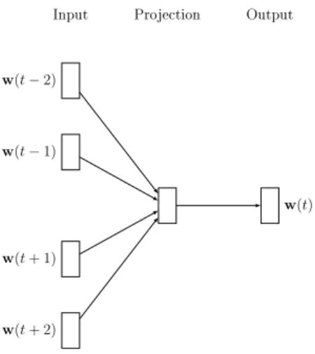
Figure 2.2: The structure of multi-word Continuous Bag of Words model
[5]. In other words, there is only one bit equals to 1and all other bits are0. We use aV ∗N matrix to represent the weight matrixW between the input and the hidden layers. We also usexandhto denote the input and hidden layer respectively. To calculate the hidden layer, simply use the following Equation 2.1:
h =xTW. (2.1)
From hidden layer to output, there is another weight matrixW0, which is dierent from W. The size of matrix W0 isN∗V. We use the following Equation 2.2 to calculate each output layer:
uj =v0wTj∗h. (2.2)
Then we can apply SoftMax function to get the posterior distribution of words and the highest probability case is assigned to the output [5]. The Equation 2.3 is the SoftMax function: p(wj|wI) =yj = exp(uj) PV j0=1exp(uj0) . (2.3)
Output w(t−2) w(t−1) w(t+ 1) w(t+ 2) Projection Input w(t)
Figure 2.3: The structure of Skip-gram model
As for multi-word context, it is similar to single-word context but we need to consider all words in the context. The Figure 2.2 shows the structure of multi-word Continuous Bag of Words (CBOW):
h= 1
CW∗(x1 +x2+...+xC). (2.4) The Equation 2.4 denes how to get the hidden layer h in word context. For multi-word Continuous Bag of Words (CBOW), we sum up all the input vectors xi where i is
a number in the range of [1, C], multiply the weight matrix W, and divide it by C. C is the size of context which indicates how many words in the current context. The process of calculating the output layer is identical with single-word context Continuous Bag of Words (CBOW).
2.1.4 Skip-gram
The whole process of Skip-gram (SG), considered as a reversed version of Continuous Bag of Words (CBOW), are homogeneous with Continuous Bag of Words (CBOW) but only takes a single word as the input whereas several words as the output [5]. The Figure 2.3 shows the Skip-gram (SG) model:
The output of Skip-gram (SG) is not multinomial distribution but C multinomial distributions. Each output is calculated from a same weight matrixW0. we still use SoftMax function to assign the highest probability case to be the result.
2.2 Text classication models
There are several popular text classication models which are involved in our exper-iment used to make compare with our approach. Some of them are classical models such as Naïve Bayes (NB), Random forest (RF),k-Nearest-Neighbours (kNN), and Support Vec-tor Machine (SVM). Those classical models are widely used to analyze short text such as Twitter. Moreover, in recent research, Neural Networks (NN) models have been more and more important and they are widely used to analyze long text data such as blog and movie review. We will introduce those models in this Section.
2.2.1 Naïve Bayes
Naïve Bayes (NB) is known as the most uncomplicated classier in Text analysis. It is generated from Bayes theorem, a classical probability model invented by Thomas Bayes (1701-1761). Naïve Bayes (NB) is extremely easy to understanding and powerful, moreover, it assumes that all the features are reciprocally independent. Although this assumption seldom holds true due to the massive interrelations among features, Naïve Bayes usually exceeds other classiers on short text like twitter. It is because short text are sparse and contain less features' interrelations.
2.2.2 Decision Tree and Random Forest
Decision Tree (DT) is a popular tree-like classier consisting nodes and branches. Each node represents a unique feature value while each branch represents a step of decision. Any path from top to one of bottom leaves is an intact decision process. We embody the value of each node by evaluating entropy and gain information. Entropy denes how many information generated from an event. Gain information allows us to measure the degree of
classes for all sample. Therefore, we can use entropy and gain information to rank attributes and build the decision tree. The nodes of decision tree locate the attributes with the lowest entropy and highest information gain among the attributes.
Although low prediction accuracy and high variance are the problem of decision tree, those drawbacks are solved by Random forest (RF). Unlike decision tree algorithm (DT), the rst step of Random Forest (RF) algorithm is to apply bagging technique to generate several small datasets. For each small dataset, the algorithm generates an unique decision tree. When the algorithm learns the dataset, inputs will go through all decision trees and the highest frequent outcome will be assigned to the nal result.
2.2.3
k
-Nearest-Neighbours
k-Nearest-Neighbours (kNN) is a representative of non-parametric lazy learning al-gorithm. "Non-parametric" indicates it doesn't make supposition on the distribution of dataset. Lazy means it doesn't have any generalization and no explicit training phase which makes algorithm pretty quickly. The core ofk-Nearest-Neighbours (kNN) algorithm is that it checks out the rstk closest neighbours of the input object and assigns the highest frequent case to the object.
2.2.4 Support Vector Machine
Support Vector Machine (SVM) are supervised machine learning algorithm which is used for both classication and regression. The aim of Support Vector Machine (SVM) is to nd a hyperplane which divides dataset into two parts. Although there is an innite volume of hyperplanes in the middle of two classes, Support Vector Machine (SVM) calculate the hyperplane which divides two groups as wide as possible. To do so, we introduce one positive hyperplane and one negative hyperplane. All of them are parallel to the decision boundary. The following Equations 2.5 and 2.6 represent the two hyperplanes:
w0+wTxneg =−1. (2.6)
The w0 is an intercept, wT is a vector, xpos and xneg are positive supported vector and
negative supported vector respectively. After combining the two Equations 2.5 and 2.6, we can get:
wT(xpos−xneg) = 2. (2.7)
We can regulate it basing on the size of the vector, and here comes the denition: w, which is dened as follows: |w|= v u u t m X j=1 w2j, (2.8)
now what we can get is as follows:
wT(xpos−xneg)
(|w|) = 2
(|w|). (2.9)
On the left part, the meaning of it indicates the distance between the two hyperplanes. It shows the margin which is treated as the target we need to maximize.In this way, we need to optimize this margin. Under this circumstance, we can make the right part 2
|w| to be
largest under the following constraint:
w0+wTxi ≥1 if yi = 1, (2.10)
w0+wTxi ≤1 if yi =−1. (2.11)
The above Equation 2.10 and Equation 2.11 conne that all data with a negative label should not transgress the negative hyperplane and for those data with a positive label should not transgress the positive hyperplane. To be concise, we combine those Equations into one
Equation which is as follows:
yi(w0+wTxi)≥1. (2.12)
For the Radial Basis Function Kernel (RBF kernel), the function is as follows: k(xi,xj) = exp(−
(xi−xj)
2(θ2) ). (2.13)
xi and xj represent two samples of dataset while θ is a free parameter. When considering
degree-d polynomials kernel function, the following Equation shows the denition:
k(xi,xj) = (xixjT+w0)d. (2.14)
The term kernel can be expressed as a similarity function between a pair of samples. The minus sign inverts the distance measure into a similarity score because we calculate the exponential of each instance, and that is the reason why all the outcome can be conned in the scale between 0 and 1 for homogeneous instances and heterogeneous instances.
The decision function of hyperplane is fully specied by a very small subset of training samples, which lies closely to the decision surface, and those training samples are called support vectors. Although dierent kernel functions have dierent algorithm, the main goal is same that calculates the hyperplane which separates support vectors as wide as possible. Linear function, Sigmoid function, Polynomial function as well as Radial basis function will be exploited as comparisons with our multi-way Factorization Machine (FM) approach.
2.2.5 Neural Networks
Neural Networks (NN) is a set of complex network-shape complex models which is highly welcomed to be used as research object among numbers of areas. Neural Networks models are made of a bunch of neural units, and the computations among them are similar
Input x1 x2 x3 +1 Projection sum Output hW(x)
Figure 2.4: The structure of a single neural unit which includes 3 inputs: x1, x2, x3, one constance, and one output: hW(x)
to the behavior of axons in brains. The units among networks are linked with each other resulting in the outcome from the previous units can be passed to the following units. The Figure 2.5 shows a simple neural unit.
The networks which stand for weights are represented by the branches. To get the value of a unit, we simply sum up the value of every branch. After that, we use the value of unit to plug in activation function. There are many activation functions such as sigmoid function, tanh function, and linear function. The following is an Equation of a general sigmoid function:
f(x) = 1
1 + exp(−x). (2.15) When we only consider one single unit, the computation of it is homogeneous with the computation of logistic regression. The output of activation function will be the input of next layer's activation function. The outputs can be expressed as :
hW(x) =f(WTx) = f(
3 X
i=1
wixi +w0). (2.16)
We can also nd that a single unit is the prototype of logistic regression and Neural Networks (NN) is made of a bunch of logistic regression.
x1 Input #1 x2 Input #2 x3 Input #3 x4 Input #4 h1 h2 h3 h4 h5 y0 Output Hidden layer Input
layer Outputlayer
Figure 2.5: The structure of a general Neural Networks (NN) model
The Figure 2.5 shows a structure of a general Neural Networks (NN). We can nd that for the input layer, there are three inputs and one bias units. The rightmost layer is called output layer and the middle layer is called hidden layer. we can use the following Equations to explain the calculation.
x(l+1)=f(W(l)x(l)). (2.17)
By using Equation 2.17, we can nally get the value of output. We name this pro-cedure forward propagation. Then basing on selected activation function such as sigmoid function, we can calculate the value of those following units. when we consider training the following dataset(x(1), y(1)), ,(x(m), y(m))ofmtraining examples. Batch gradient descent is a good choice to be applied in our Neural Networks (NN). To be more specic, for a single training instance(x, y), after applying the cost function we dened, we can reach the below Equation:
J(W;x, y) = 1
2(|hW(x)−y|)
2
. (2.18)
The loss function is made of two parts. For the rst part, it is an average sum-of-squares error term. While the last term is used to penalize the rst term so that to avoid overtting.
Moreover, by tuning the parameters, we can easily adjust the relative signicance between the two terms. Note also the small overloaded notation: J(W;x, y) is the squared error cost with respect to a single example; To sum up, J(W) is a general cost function with the penalty term. To learn the pattern, we need to make it as small as possible. To train our Neural Networks (NN), rst of all, we will randomly set a low value on each term in the Equation. Next, we will apply batch gradient descent to optimize the parameters among networks. Although it is a non-convex function and sometimes it will return a local optimal value, it is widely used and has a steady performance in reality. Last but not least, it should be a random fashion for initialization and the more variety, the better. Otherwise, the learning process is meaningless, and that is the reason why we need to initialize those values randomly. For each epoch, the parameters are updated basing on the following pseudocode:
W(ijl) =Wij(l)−α ∂ ∂Wij(l)J(W)
, (2.19)
where α is the learning rate. The most signicant thing is to calculate the gradient on each term. In our experiment, we use Theano package to implement the Deep Neural Networks (DNN). We use a 4-layer Deep Neural Networks (DNN) including 2 hidden layers to make comparison with our multi-way Factorization Machine (FM) approach. Moreover, there are 600 units in the rst hidden layer while there are 300 units in the second hidden layer. We try three dierent activation functions including sigmoid function, tanh function, and linear function and we will choose the one which results in best performance.
2.3 Sentiment analysis methods
There are numbers of sentiment analysis approaches in machine learning area. Naïve Bayes (NB), Random Forest (RF), k-Nearest-Neighbours (kNN), as well as Support Vector Machine (SVM) are widely used in previous researches while Neural Networks (NN) models are widely used in current researches.
2.3.1 Earlier research
[13] is a paper with the aim to identify a movie review as "thumbs up" or "thumbs down". In their research, popular classication models including Naïve Bayes and Support Vector Machine are examined to the sentiment classication problem. The dataset is from Internet Movie Database (IMDb) with two categories: positive and negative. In total, the dataset consists 1301 positive reviews and 752 negative reviews. All reviews are written by 144 reviewers. Their result demonstrates the feasibility that using Naïve Bayes (NB) and Support Vector Machine (SVM) models to do sentiment analysis.
In [11], they elaborate Support Vector Machine (SVM) approach to do sentiment analysis. Dierent from general SVMs, they invent hybrid SVMs which combines feature embedding method with general SVMs. Their conclusion demonstrates hybrid SVMs can provide robust performance on short text dataset. Nevertheless, their approach cannot generate robust result on long text dataset.
In [3], they propose a graph-based semi-supervised learning algorithm to address the task of inferring numerical ratings for unlabelled documents based on the perceived sentiment expressed by text. The model they invent has the similar structure withk -Nearest-Neighbours (kNN). The dataset they use is Twitter data. Their conclusion demonstrates that their graph-based semi-supervised learning algorithm is feasible on short data. However, their approach cannot generate robust outcomes on large labelled dataset.
In [2], the authors propose a hierarchical tree model which can be extended to analyze any number categories classication problem. To be more specic, they combine decision tree with SVMs and use Kruskal's algorithm to calculate and reduce the runtime. The dataset they use is same with the dataset used in [3]. Although the experiment result is not bad, the drawback is that their approach didn't combine any preprocessing methods.
The drawback of earlier researches is that they only focus on short text dataset such as Twitter but ignore long text data such as blog. However, there are numbers of recent
sentiment analysis approaches which are used to analyze long text such as movie review and they are based on Neural Networks (NN) model.
2.3.2 Recent research
In a pioneering study [16], authors proposed a Recursive Neural Tensor Networks model that aims to overcome the limitation of context-free Bag of Words (BOW) for ana-lyzing longer textual data. In their model, each word is assigned to a node and represented by a vector. The value of each parent node is generated using their children nodes as input through activation of a SoftMax function. In this way, this approach is context-based as opposed to concentrating on discrete words. However, the interior noise is not appropriately handled that substantially undermines the performance. Further, the training process is also challenged by vanishing and exploding gradient problems in optimization [5].
In [8], authors proposed a gated Recurrent Neural Networks sentiment classication model. Since the gate mechanism is exploited in each neural unit, those inputs that are not over the threshold are set by the gate as noise and ltered out to simplify the training process. This approach is nevertheless not scalable for big textual data [5].
A more computational ecient approach is proposed in [6], where the algorithm applies Dynamic k-Max Pooling. It is an operation among linear sequences. The algorithm only considers rst k-th maximum values in the sequence so that the runtime and noise are reduced and ltered out respectively. Moreover, the parameter k can be dynamically chosen by making it a function of other aspects of the network or the input. However, the remaining issue is that the input is unweighted leading to inaccurate outcomes [5].
To address the unweighted issue, in [1], authors proposed a top-down document level sentiment analysis approach, which reweighs the factor of each phrase unit basing on its order in a context representation of the sentence structure and the factor can generate from a naïve function or tun from a partial part of the dataset. Specically, they used dependency based phrase tree formulation to convert their constituent-like RST tree into a directed graph
over elementary discourse units. Then, they constructed a naïve linear function to learn the factor to each item. However, their approach has two drawbacks. First, a simple linear reweighting function is insucient to satisfy a variety of massive textual data. Second, since unlabelled datasets are more common, to invent a semi-supervised machine learning model is necessary. The following approach is a semi-supervised machine learning model [5].
In [7], they put forward a semi-supervised bootstrapping approach to learn the rela-tionship between Chinese government and foreigners basing on the "People's daily". More-over, dierent from other approach, their approach considers time information as one ele-ment to analysis and they use a hierarchical Bayesian model. It is novel to take newspaper as dataset to do sentiment analysis. Their approach evolves in the following three steps: First, expression and target are extracted from sentiment related terms by semi-Markov Conditional Random Fields algorithm. Next, notations including sentiment score, document target list and sentence list are introduced to mark information extracted from the rst step. Finally, Semi-supervised Bootstrapping method is applied in Hierarchical Bayesian Markov Model to train the dataset.
The above-mentioned sentiment analysis approaches, although eective, are all de-signed for longer textual documents. Thus, new approaches that are scalable, easy to train and tune to accommodate both longer and shorter textual data are needed [5].
2.4 Evaluation method
We exploit Area Under the receiver operating Curve (AUC) as the evaluation method of the performance of dierent sentiment analysis methods. Receiver operating curve (ROC) is a curve widely used to demonstrate the achievement of a binary classier system with a range of threshold from 0 to 1. For each method, ROC curve is made of pairs of True Positive Rate (TPR) and False Positive Rate (FPR). [5]. We dene the TPR and FPR based on the following Table 2.1. The TRUE and FALSE values in the rst column represent the results in reality, while the TRUE and FALSE values in the rst row represent the prediction
Table 2.1: Confusion matrix Table
AUC Performance
TRUE FALSE
TRUE TP:true positive FP:false positive FALSE TN:True negative FN: false negative
Table 2.2: AUC value reference Table
AUC Performance
0.5 No discrimination
[0.7,0.8) Acceptable discrimination [0.8,0.9) Excellent discrimination
[0.9,1] Outstanding discrimination (but extremely rare)
results. TP, FP, FN, TN mean the number of results in each permutation of the results. The TPR and FPR are dened as the following Equations:
T P R= T P
T P +F N , (2.20)
F P R = F P
F P +F N . (2.21)
AUC is calculated by integrating ROC curve in the range from 0 to 1 [4]. A method with large AUC value means that it achieves high TPR at very low FPR, thus is superior to the competing methods [5]. The Table 2.2 shows the performance corresponding with a detailed AUC score.
CHAPTER 3: MULTI-WAY FM METHOD
Recently, factorization models have been more and more important in much research in the area of machine learning. From a variety of implementations and applications, we nd that they have the superior capabilities in a range of elds such as recommender systems [15]. The most well-studied factorization model is matrix factorization. It makes algorithm feasible to learn the interrelation among features. It has been applied to multiple domains such as healthcare [14] and social science [18].
In this thesis, FM [15] is presented. FM has excellent accuracy basing on factorization models as well as exibility. Homogeneous to other text classication models including Random Forest (RF) and Support Vector Machine (SVM), the input text of FM are made of real features. The dierence between FM and other classication models is that instead of other models, FM use a factorized fashion to represent the interrelations among features. Moreover, when dealing with sparse features such as healthcare, FM can achieve excellent performance. It has proven that the factorized style is feasible to simulate the interactions by algorithm learning [15]. We can dene that for any learning problem, it is illustrated by a design X ∈ Rn∗p. The ith row x
i ∈ Rp of X describes one instance with p real features
and where yi is the target of the ith instance. In other words, It is also make sense that to
illustrate this collection as a set S of tuples (x, y), where x∈Rp is a feature vector and y is
the corresponding target. The combination style that both data matrices and the feature are considered together is widely used in the area of machine learning such as logistic regression or Naïve Bayes (NB).
3.1 Two-way FM
The special case of two-way FM that captures pair-wise feature interaction is de-scribed as below: ˆ y(x) :=w0 + n X i=1 wixi+ n X i=1 n X j=i+1 hvi,vjixixj. (3.1)
It learns the relation of unary feature relations and binary feature interrelations with sentiment label. The left part of the Equation is a linear regression model, which contains the unary feature relations. The rest of the Equation is nested sums includes all features' interrelations which represent the binary interrelations. The signicant dierence between FM and general polynomial regression algorithm is that FM approach exploit a factorized fashion to value those parameters so that to calculate the interrelation between each feature, rather than using an independent parameter. This meaningful character allows FM to ana-lyze data even it is highly sparse where popular models can not generate excellent outcome. The second part combines two nested sums includes all binary interactions among features, that is, xixj [5]. The important dierence to general polynomial regression is that the
in-terrelation is not dened by an independent term wj,j but with a factorized parametrization
wj,j = n X i=1 n X j=i+1
h vi,vjixixj which demonstrates the rank of the binary interrelation is low.
Under this circumstance, unlike other models which can not generate excellent performance among sparse data, FM can learn and simulate the relation among sparse data. w0 ∈ R
is global intercept and w ∈ Rn models the contribution of i-th feature to the sentiment
label. vi represents the i-th feature with k factors, which is a hyper-parameter that denes
the dimensionality of factorization of W. Since all the pairwise features are dependent, the feature interaction can be estimated with sparse observation in the corresponding pairs. For example,hvi,vjirelates tohvi,vliin terms of vi. Data for one pairwise interaction facilitates
the parameter estimation of related pairwise interactions. The parameter n is the length of output for each input sentences, in other words, n is the column number of matrix. After using feature embedding and representing methods, it will return a sequence with length of n which relates to the weights of the rst n most frequent key words. In this Principal components analysis (PCA) way, instead of learning the original matrix which could be very wide, new input matrix could be thinner than the original. The parameter vi is a vector
dedicated to the i-th feature with size ofk. k represents the dimension of word vectors em-bedding, which is a tuning parameter that could be adjusted for shorter and longer textual
data. Specically, we tunek to smaller values for more sparse feature (word) vectors such as those from shorter Twitter text and we tune k to larger values for less sparse feature (word) vectors from longer movie review documents. The author proposed an Equation to shrink the runtime from O(kn2)to O(kn), the Equation is as follows:
n X i=1 n X j=i+1 hvi,vjixixj = 1 2 k X f=1 (( n X i=1 vi,fxi)2− n X i=1 vi,f2 x2i). (3.2)
3.2 Features' interaction
Table 3.3: User movie review record Table
User Movie Other Movies rated Time Last Movie rated Target
A B C TI NH SW ST TI NH SW ST Time TI NH SW ST y 1 0 0 2 0 0 0 0.3 0.3 0.3 0 13 0 0 0 0 5 1 0 0 0 1 0 0 0.3 0.3 0.3 0 14 1 0 0 0 3 1 0 0 0 0 1 0 0.3 0.3 0.3 0 16 0 1 0 0 1 0 1 0 0 0 1 0 0 0 0.5 0.5 5 0 0 0 0 4 0 1 0 0 0 0 1 0 0 0.5 0.5 8 0 0 1 0 5 0 0 1 1 0 0 0 0.5 0 0.5 0 9 0 0 0 0 1 0 0 1 0 0 1 0 0.5 0 0.5 0 12 1 0 0 0 5 The term n X i=1 n X j=i+1
h vi,vjixixj expresses the features' non-linear interaction [5]. To
introduce the concept of non-linear interaction, the Table 3.3 is an example. Table 3.3 contains user-moive rate information. Every row is a independent record including user name information, movie name information, movies rated information, and time information. Target is corresponding score of each record. Supposed that we want to get the score of movie ST given by user A, we can hardly nd the answer because there isn't any records containing A with movie ST. However, if we use FM, we can calculate the interaction by factoring it so that the result is more accurate. Think about the user B and C, they have almost the same score of movie SW. So we can infer some vectors of them should be positive correlative. Now, let us consider the User A and C, A gives movie TI 5 and gives movie SW 1 while C gives movie TI 1and gives movie SW 5. So we can infer vectors of them should be negative
correlative. Next, since B gives similar socre to movie SW and ST, so the vector of movie SW and ST should also have some similarity. Finally, we can make conclusion that the score of ST will similar to the score of SW. By using FM, all the vectors can be calculated by factoring them, and the interrelations can be calculated by vector's dot product.
3.3 Learning FM
Input: Training data S, penalty term λ, learning rate η, initialization σ Output: Model parameters Θ = (w0,w,V)
w0 ←0;w←(0, . . . ,0);V ∼ N(0, σ); repeat for (x, y)∈S do w0 ←w0−η( ∂ ∂w0 l(y(x|Θ), y) + 2λ0w0); for i∈ {1, . . . , p} ∧xi 6= 0 do wi ←wi−η( ∂ ∂wi l(y(x|Θ), y) + 2λwπwi); for f ∈ {1, . . . , k} do vi,f ←vi,f −η( ∂ ∂vi,f l(y(x|Θ), y) + 2λvf,π(i)vi,f); end end end
until stopping criterion is not met;
Algorithm 1: Stochastic Gradient Descent (SGD)
In this thesis, we concentrate on Stochastic gradient descent (SGD) way to learn FM. SGD algorithm is widely used for tuning parameters in machine learning area. It is easy to implement and generate steady outcome among dierent loss functions, and the runtime cost and space cost are inexpensive. The algorithm take loops basing on S and renew every parameters by updating them.
Θ←Θ−η( ∂
The meaning of η is the learning step for SGD algorithm. The performance of the SGD is sensible with the size of the learning step. If it is too big, the result can hardly converge while if ti si too small, the process of learning will be slow.
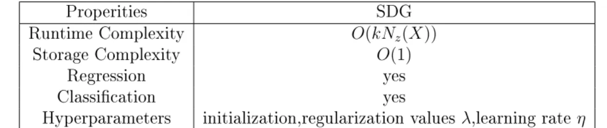
In general, we should rst dene the value of η. Then,we dene λ, a penalty term to regulate the algorithm. Î is the value of the corresponding feature and (V) need to be randomly initialized. Here is a Table shows the properties of the Learning Algorithm:
Table 3.4: Properities of the Stochastic Gradient Descent (SGD) Learning Algorithm
Properities SDG
Runtime Complexity O(kNz(X))
Storage Complexity O(1)
Regression yes
Classication yes
Hyperparameters initialization,regularization values λ,learning rate η
3.4 Multi-way FM
The two-way FM model can be further generalized to multi-way FM model to accom-modate higher-order feature interactions as follows [15]:
ˆ y(x) := w0+ n X i=1 wixi + d X m=2 n X i1=1 ... n X im=im−1+1 ( m Y j=1 xij)( km X f=1 m Y j=1 v(im) j,f). (3.4)
The multi-way FM models higher-order interactions among feature vectors ofkfactors instead of full n feature (word) vectors. Likewise, m, representing the order of FM models, is also a tunning parameter that can be adjusted for shorter Twitter text and longer movie review textual data. For more sparse Twitter text, a two-way FM model, i.e., m = 2, is sucient for estimating non-linear feature interaction and higher-order FM models (larger m) might not help much. For less sparse textual data, a larger m may better capture the higher-order feature interactions, particularly for big data [5].
3.5 Summary
FM models have exibility in the area of machine learning basing on the factorized pattern. In this chapter, we introduced the current research basing on FM models and the SGD algorithm, to be more specic, we make emphasis on the meaning of parameters and the expressiveness. It is proven that FM models can simulate specic factorization patterns but not limit to those patterns. Numbers of results demonstrate that the outcome of the described algorithm for FM models are as excellent as other popular models in the eld of recommender system,
In total, the main advantages of multi-way FM models are: (1) interactions between feature vectors can be estimated especially for very sparse feature vectors; (2) the number of parameters and the running timeO(kn)are linear, which make Stochastic Gradient Descent (SGD) training feasible and scalable [15]. In our experiments, we investigate the performance of FM models by tunning parameters k and m [5].
CHAPTER 4: Experiments
In this chapter, we will rst introduce the methodology, which describes the detailed process of our experiments. Next, we will illustrate the rst experiment, the aim of which is to seek the optimal parameter k. We will use short twitter dataset and long movie review dataset. For both datasets, we will nd a corresponding optimal k. After that, we will describe the second experiment, the aim of which is to seek the optimal parameterm, using optimal k generated from the rst experiment on both twitter dataset and movie review dataset. Then, we will use optimalk and optimal mgenerated from the second experiments to do the training and make prediction. In order to show the performance of multi-way FM, we will also use other sentiment analysis approaches and make comparison with our result [5].
4.1 Methodology
We carried out our experiments in two steps. First, in order to recognize human natural language, we used feature representation (e.g. Bag of Words) or embedding (e.g. Continuous Bag of Words and Skip-gram) to convert textual data to feature matrix, which is amenable for machine learning methods. Second, we used FM to learn the relationship between embeded features and the corresponding sentiment label considering higher-order feature interaction. In order to demonstrate the robust performance of FM for both shorter and longer textual data, we explored a wide range ofk andm values [9]. We use Area Under the receiver operating Curve (AUC) as the metric for evaluating the performance of dierent sentiment analysis methods. For each method, Receiver Operating Characteristic (ROC) curve is plotted using the pairs of True Positive Rate (TPR) and False Positive Rate (FPR). AUC is calculated by integrating ROC curve in the range from 0 to 1 [4]. A method with large AUC value means that it achieves high TPR at very low FPR, thus is superior to the competing methods [5]. The following owchart 4.1 shows the process of our approach:
Start
Input
Short text?
Smallk, smallm Largek, largem
Multi-way FM
Output
Stop
yes no
Figure 4.1: The procedure of our multi-FM approach
4.2 Datasets
To demonstrate the robust performance of FM for both longer and shorter tex-tual data, we performed sentiment analysis on a Twitter data set from https://inclass. kaggle.com/c/si650winter11/download and movie review data set from https://www. kaggle.com/c/word2vec-nlp-tutorial/download/labeledTrainData.tsv.zip. The for-mer has 7086 tweets while the latter has 25000 movie reviews [5]. The following two gures shows the detailed information of two datasets.
Twitter data are shown in 4.2 while movie review data are shown in 4.3. For both cases, we focus on binary sentiment analysis with a sentiment label of either 0 or 1.
4.3 Model tunning with
k
We rst demonstrate the exibility of FM to diverse textual data by tunning the parameter k. We explored performance of the two-way FM using a range of k values from 2
Figure 4.2: The length distribution of Twitter data
to 20. For each k and for each data set, we calculated AUC values to observe the trend and to select the optimal k. For feature representation, we use Bag of Words (BOW) for more sparse Twitter data and Continuous Bag of Words (CBOW) for less sparse movie review textual data. It is because the longer movie review text makes it possible for Continuous Bag of Words to consider the context of the word. On the contrary, the context-free Bag of Words may work better for shorter Twitter text [5].
From the Figure 4.4 we nd that for both Twitter and movie review data, they demonstrate a similar trend, i.e., performance of the FM approach rst increases with the increasing k values, and then decreases for larger k values.
By tuning parameterk, FM provides the distinguished performance for twitter dataset and blog dataset with the optimalk=6 and k=16 respectively. It conrmed our notion that using smaller k values for classifying shorter Twitter text and larger k values for classifying longer text. By tuning the single parameter k, FM achieved a robust performance for both Twitter and movie review data. Those optimal k are involved in the next experiment in order to seek the best m [5].
Figure 4.3: The length distribution of movie review data
4.4 Model tunning with
m
We continue to test the performance of multi-way FM by tunning the parameter m in the range from 2 to 10. Similarly, we used BOW for Twitter text (k = 6) and CBOW for movie review text (k = 16). In Figure 4.5, the performance of multi-way FM using Twitter data is not sensitive to the choice of m values. For longer movie review data, multi-way FM performs better than two-way FM and remains similar for a number of larger values of m before it drops. In summary, the performance of multi-way FM is relatively stable over the choice of m, thus k remains as the single tuning parameter that would achieve robust performance across a variety of textual data [5].
4.5 Method comparison
Using both Twitter and movie review data, we compared FM with an array of baseline and newer classiers, e.g., Naïve Bayes (NB), Random Forest (RF), k-Nearest-Neighbours (kNN), Deep Neural Networks (DNN), and Support Vector Machine (SVM). For DNN, we used an architecture of 4 layers including 2 hidden layers with 600 neurons in the rst hidden layer and 300 neurons in the second layer. For SVM's, we tested four popular kernel functions
Figure 4.4: The robust performance of our multi-way FM approach achieved by tunning a single parameter k
including radial basis function, linear function, sigmoid function and polynomial function. In Table 4.5, we run each experiment three times and report the average AUC value and the corresponding variance in the parenthesis. The multi-way FM achieves the best performance (bold faced) in both Twitter (m= 5) and movie review (m= 7) data among all the selected sentiment analysis methods. Note from Figure 4.5, the superior performance of the multi-way FM approach remains stable for other choices of m values. The source code of our analysis is available from the corresponding author's website [5].
Figure 4.5: The robust performance of our multi-way FM approach achieved by tunning a single parameter m
Table 4.5: Performance comparison
Twitter movie review
Classier Bag of Words Continuous Bag of Words Bag of Words Continuous Bag of Words NB (0.005)0.965 (0.035)0.719 (0.007)0.675 (0.003)0.797 RF (0.002)0.971 (0.007)0.951 (0.001)0.682 (0.029)0.764 kNN 0.968 0.938 0.624 0.784 (0.001) (0.003) (0.001) (0.012) RBFSVM (0.003)0.966 (0.045)0.565 (0.005)0.693 (0.006)0.714 LinearSVM (0.002)0.970 (0.018)0.861 (0.004)0.696 (0.011)0.839 SigmoidSVM (0.001)0.943 (0.005)0.839 (0.007)0.586 (0.010)0.837 PloySVM (0.002)0.964 (0.008)0.613 (0.040)0.638 (0.001)0.701 DNN (0.008)0.767 (0.025)0.820 (0.006)0.743 (0.001)0.837 FM (0.001)0.990 (0.008)0.929 (0.001)0.677 (0.011)0.840
CHAPTER 5: CONCLUSION
5.1 Summary of Contributions
In this thesis, we illustrated our multi-way Factorization Machine approach for sen-timent analysis. Our multi-way Factorization Machine approach can not only analyse short Twitter data but also analyse long movie review data. For short Twitter dataset, we use Bag of Words (BOW) to be the feature representation method while for long movie review dataset, we use Continuous Bag of Words (CBOW) to be the feature embedding method. Moreover, we use two adjustable parametersk (the length of vector) andm(the degree of Factorization Machine) to pursue the best performance. For Twitter dataset, the optimal k equals 6 and optimalmequals 5. For movie review dataset, the optimalkequals 16 and optimalm equals 7. Basing on those optimal parameters, the AUC value on Twitter dataset is 0.99 and the AUC value on movie review dataset is0.84, which exceeds other comparison including Naïve Bayes (NB), Random Forest (RF),k-Nearest-Neighbours (kNN), Linear Support Vector Ma-chine (LinearSVM), Sigmoid Support vector MaMa-chine (SigmoidSVM), Polynomial Support Vector Machine (PolySVM), Radial basis Support Vector Machine (RBFSVM), and Deep Neural Networks (DNN). We apply Bag of Words (BOW) to Twitter dataset while apply Continuous Bag of Words (CBOW) to movie review dataset. After comparing with other approaches, we make conclusion that: By tuning parameter k, our multi-way Factorization Machine is one of the best approach for sentiment analysis.
5.2 Future Research Directions
For future studies, we will extend the supervised multi-way FM to semi-supervised framework, which can be used to analyze textual data with incomplete sentiment labels. Also, we will extend our binary model to multi-categories model to learn multi-categories dataset.
REFERENCES
[1] P. Bhatia, Y. Ji, and J. Eisenstein, Better document-level sentiment analysis from rst discourse parsing, arXiv preprint arXiv:1509.01599, 2015.
[2] A. Bickerstae and I. Zukerman, A hierarchical classier applied to multi-way senti-ment detection, in Proceedings of the 23rd international conference on computational linguistics. Association for Computational Linguistics, 2010, pp. 6270.
[3] P. Chaovalit and L. Zhou, Movie review mining: A comparison between supervised and unsupervised classication approaches, in System Sciences, 2005. HICSS'05. Pro-ceedings of the 38th Annual Hawaii International Conference on. IEEE, 2005, pp. 112c112c.
[4] J. A. Hanley and B. J. McNeil, The meaning and use of the area under a receiver operating characteristic (roc) curve. Radiology, vol. 143, no. 1, pp. 2936, 1982. [5] Jingwei and D. Zhu, Multi-way factorization machine for sentiment analysis, in
EMNLP, 2017.
[6] N. Kalchbrenner, E. Grefenstette, and P. Blunsom, A convolutional neural network for modelling sentences, arXiv preprint arXiv:1404.2188, 2014.
[7] J. Li and E. H. Hovy, Sentiment analysis on the people's daily. in EMNLP, 2014, pp. 467476.
[8] B. Liu, Sentiment analysis and opinion mining, Synthesis lectures on human language technologies, vol. 5, no. 1, pp. 1167, 2012.
[9] A. N. Mikhail Tromov, tm: Tensorow implementation of an arbitrary order factor-ization machine, https://github.com/gey/tm, 2016.
[10] T. Mikolov, K. Chen, G. Corrado, and J. Dean, Ecient estimation of word represen-tations in vector space, arXiv preprint arXiv:1301.3781, 2013.
[11] T. Mullen and N. Collier, Sentiment analysis using support vector machines with diverse information sources. in EMNLP, vol. 4, 2004, pp. 412418.
[12] B. Pang, L. Lee et al., Opinion mining and sentiment analysis, Foundations and TrendsR in Information Retrieval, vol. 2, no. 12, pp. 1135, 2008.
[13] B. Pang, L. Lee, and S. Vaithyanathan, Thumbs up?: sentiment classication using machine learning techniques, in Proceedings of the ACL-02 conference on Empirical methods in natural language processing-Volume 10. Association for Computational Linguistics, 2002, pp. 7986.
[14] I. Perros and J. Sun, Factorization machines as a tool for healthcare: Case study on type 2 diabetes detection, 2015.
[15] S. Rendle, Factorization machines, in Data Mining (ICDM), 2010 IEEE 10th Inter-national Conference on. IEEE, 2010, pp. 9951000.
[16] R. Socher, A. Perelygin, J. Y. Wu, J. Chuang, C. D. Manning, A. Y. Ng, C. Potts et al., Recursive deep models for semantic compositionality over a sentiment treebank, in Proceedings of the conference on empirical methods in natural language processing (EMNLP), vol. 1631. Citeseer, 2013, p. 1642.
[17] D. Tang, B. Qin, and T. Liu, Document modeling with gated recurrent neural network for sentiment classication. in EMNLP, 2015, pp. 14221432.
[18] M.-F. Tsai, C.-J. Wang, and Z.-L. Lin, Social inuencer analysis with factorization machines, in Proceedings of the ACM Web Science Conference. ACM, 2015, p. 50.
ABSTRACT
MULTI-WAY FACTORIZATION MACHINE FOR SENTIMENT ANALYSIS by
JINGWEI ZHANG MAY 2017 Advisor: Dr.Dongxiao Zhu
Major: Computer Science Degree: Master of Science
Sentiment analysis is a process of learning the relationship between sentiment label and text. The research value of sentiment analysis is two-fold: rst, it has a wide range of applications in many sectors and industries, e.g., the industry has ourished due to the proliferation of commercial applications such as using sentiment analysis as an integrated part of customer experience strategy. Second, it oers an array of new challenging problems for research community such as word feature embedding and machine learning. Albeit ear-lier methods such as Naïve Bayes (NB), Random Forest (RF),k-Nearest-Neighbours (kNN), Support Vector Machine (SVM) and more recent methods such as Deep Learning (DL) methods are eective, they are primarily designed for shorter or longer textual data thus are not able to maintain a robust performance across a variety of text with diverse lengths. In reality, some text is as abbreviated as one single word while others are so pleonastic that are over thousands of words. Moreover, ad hoc combination of feature embedding and learning methods makes it more dicult to choose the right approach for dierent types of textual data. Undoubtedly an integrated feature embedding and sentiment analysis method is desirable. In this thesis, we introduce multi-way FM as a new method for sentiment anal-ysis accounting for higher-order feature interaction. We demonstrate the performance and exibility of the FM method to other competing methods by tuning a single parameter to accommodate both shorter Twitter and longer movie review documents.
AUTOBIOGRAPHICAL STATEMENT
Jingwei Zhang is a Master student majoring in Computer Science in Wayne State University. Before that, he got his Bachelor degree of Computer Science in Xidian University.