Deep Learning for Detection and Segmentation in High-Content Microscopy Images

(1)

DISSERTATION

submitted

to the

Combined Faculty for the Natural Sciences and Mathematics

of

Heidelberg University, Germany

for the degree of

Doctor of Natural Sciences

Put forward by

Thomas Sebastian Wollmann, M.Sc.

Born in: Solingen, Germany

Oral examination: ...

(2)

(3)

Deep Learning for Detection and Segmentation in

High-Content Microscopy Images

(4)

(5)

Abstract

High-content microscopy led to many advances in biology and medicine. This fast emerging technology is transforming cell biology into a big data driven science. Computer vision methods are used to automate the analysis of microscopy image data. In recent years, deep learning became popular and had major success in computer vision. Most of the available methods are developed to process natural images. Compared to natural images, microscopy images pose domain specific challenges such as small training datasets, clustered objects, and class imbalance.

In this thesis, new deep learning methods for object detection and cell segmentation in microscopy images are introduced. For particle detection in fluorescence microscopy images, a deep learning method based on a domain-adapted Deconvolution Network is presented. In addition, a method for mitotic cell detection in heterogeneous histopathology images is proposed, which combines a deep residual network with Hough voting. The method is used for grading of whole-slide histology images of breast carcinoma. Moreover, a method for both particle detection and cell detection based on object centroids is introduced, which is trainable end-to-end. It comprises a novel Centroid Proposal Network, a layer for ensembling detection hypotheses over image scales and anchors, an anchor regularization scheme which favours prior anchors over regressed locations, and an improved algorithm for Non-Maximum Suppression. Furthermore, a novel loss function based on Normalized Mutual Information is proposed which can cope with strong class imbalance and is derived within a Bayesian framework.

For cell segmentation, a deep neural network with increased receptive field to capture rich semantic information is introduced. Moreover, a deep neural network which combines both paradigms of multi-scale feature aggregation of Convolutional Neural Networks and iterative refinement of Recurrent Neural Networks is proposed. To increase the robustness of the training and improve segmentation, a novel focal loss function is presented.

In addition, a framework for black-box hyperparameter optimization for biomedical image analysis pipelines is proposed. The framework has a modular architecture that separates hyperparameter sampling and hyperparameter optimization. A visu-alization of the loss function based on infimum projections is suggested to obtain further insights into the optimization problem. Also, a transfer learning approach is presented, which uses only one color channel for pre-training and performs fine-tuning on more color channels. Furthermore, an approach for unsupervised domain adaptation for histopathological slides is presented.

Finally, Galaxy Image Analysis is presented, a platform for web-based microscopy image analysis. Galaxy Image Analysis workflows for cell segmentation in cell cultures, particle detection in mice brain tissue, and MALDI/H&E image registration have been developed.

(6)

Abstract

microscopy image data from various microscopy modalities. It turned out that the proposed methods yield state-of-the-art or improved results. The methods were benchmarked in international image analysis challenges and used in various cooperation projects with biomedical researchers.

(7)

Zusammenfassung

High-Content Mikroskopie führte zu vielen Fortschritten in der Biologie und Medi-zin. Diese Technologie hat die Zellbiologie in eine durch große Daten getriebene Wissenschaft transformiert. Computergestützte Bildanalyse wird genutzt, um mikroskopische Bilddaten automatisiert auszuwerten. In den letzten Jahren ist Deep Learning durch die Erfolge in der computergestützten Bildanalyse populär geworden. Die meisten eingesetzten Methoden wurden für die Anwendung an Bildern von natürlichen Szenen entwickelt. Im Vergleich dazu besitzen mikroskopische Bilddaten domänenspezifische Herausforderungen wie wenig Trainingsdaten, hohe Objektdichte und Klassenungleichgewicht.

In dieser Arbeit werden neue Deep Learning Methoden für Objekterkennung und Zellsegmentierung in Mikroskopiebildern vorgestellt. Es wurde eine Methode für Partikeldetektion in Fluoreszenzmikroskopiebildern auf Basis eines für diese Anwen-dung optimierten Deconvolution Network entwickelt. Weiterhin wurde eine Methode für die Detektion von mitotischen Zellen in heterogenen histopathologischen Bildern entwickelt, welche ein Deep Residual Network mit Hough Voting kombiniert. Die Methode wird für das Grading von Whole-Slide Histologiebildern genutzt. Darüber hinaus wurde eine Methode für sowohl Partikeldetektion als auch Zelldetektion basierend auf Objektzentroiden entwickelt, welche end-to-end trainiert werden kann. Die Methode umfasst ein Centroid Proposal Network, ein Layer für die Aggrega-tion von DetekAggrega-tionshypothesen über alle Bildskalen und Anker, sowie eine Methode zur Regularisierung, die a-priori Anker gegenüber vorhergesagten Verschiebungen bevorzugt, und einen verbesserten Algorithmus für Non-Maximum Suppression. Eine neue Loss-Funktion basierend auf normalisierter Mutual Information wird vorgestellt, die mit starkem Klassenungleichgewicht umgehen kann.

Für die Zellsegmentierung wird ein Neuronales Netz mit vergrößertem rezeptiven Feld vorgestellt, um mehr semantische Informationen zu modellieren. Darüber hinaus wird ein Neuronales Netz vorgeschlagen, dass die Paradigmen von Multi-Skalen-Feature-Extraktion von Convolutional Neural Networks und iteratives Verfeinern mittels Recurrent Neural Networks verbindet. Für ein robusteres Training und eine verbessererte Segmentierung wurde eine Focal Loss basierte Loss-Funktion entwickelt.

Weiterhin wird ein Framework für Black-Box Hyperparameteroptimierung für biomedizinische Bildverarbeitungspipelines vorgestellt. Dieses Framework nutzt eine modulare Architektur, die Hyperparameterabtastung und Hyperparameterop-timierung trennt. Eine Visualisierung der Loss-Funktion, basierend auf Infimum Projektionen für die Analyse des Optimierungsprozesses, wird vorgeschlagen. Darüber hinaus wird eine Transfer Learning Technik vorgestellt, die Netzwerke, die mit einem Eingangskanal trainiert wurden, für Daten mit mehreren Eingangskanälen nutzbar macht. Zusätzlich wurde eine Methode für Unsupervised Domain Adaptation in histopathologischen Schnitten entwickelt.

(8)

web-Zusammenfassung

basierte Analyse von mikroskopischen Bildern. Galaxy Image Analysis Workflows f¨ur Zellsegmentierung in Zellkulturen, Partikeldetektion in Hirnschnitten von M¨ausen, und MALDI/H&E Registrierung werden vorgestellt.

Die vorgestellten Methoden wurden f¨ur synthetische und reale Mikroskopiedaten mehrerer Modalit¨aten angewandt und erreichten Stand der Kunst oder bessere Performanz. Die Methoden wurden in internationalen Wettbewerben evaluiert und mit Kooperationspartnern in biomedizinischen Forschungsprojekten genutzt.

(9)

Acknowledgements

Undertaking my doctoral studies in computer science at the faculty for mathematics and computer science at Heidelberg University would not have been possible without the support and guidance that I received from many people.

First of all, I would like express my great thanks to PD Dr. Karl Rohr for supervising my work, but especially for his patience and always providing me with freedom to work on the topics I am interested in.

I want to express my gratitude to all the people with whom I had very productive collaborations. A special thanks goes to Dr. Björn Grüning (Backofen lab, University of Freiburg) for integrating me into the lovely Galaxy and Bioconda communities and always helping me out at the craziest times of the day. In addition, I would also like to thank my biomedical cooperation partners Charlotte Bold (Müller lab, Heidelberg University), Dr. Delia Braun (Rippe lab, DKFZ Heidelberg), PhD Karina Durso-Cain (Uprichard lab, Loyola University Chicago), Dr. Melanie Föll (Schilling lab, University of Freiburg), Dr. Manuel Gunkel (Erfle lab, Heidelberg University), Dr. Peter Kumberger (Graw lab, Heidelberg University), Dr. Alexandra Poos (König lab, University Hospital Jena), and all the others for letting me be part of their interesting research projects.

A big thanks goes to my colleague Christian Ritter for fruitful discussions, research collaboration and being a great companion during my doctoral studies. Moreover, I would like to thank the entire Biomedical Computer Vision Group for many discussions. Especially, I want to thank our secretaries Manuela Sch¨afer and Sabrina Wetzel for always keeping everything running smoothly and to take the university bureaucracy load off us. I want to thank my supervised interns, master students, and student assistants Danny Baltissen, Patrick Bernhard, Jan-Niklas Dohrke, Sophia Eijkman, Simone Gierlich, Julia Ivanova, Roman Spilger, Hao Tian, Niklas Vockert, and Kevin Walz for labeling and supporting me carrying out the experiments.

I am very grateful that Cornelia Wollmann, Dr. Gerhard Wollmann, Sarah Linnemeier, and Sanja Miskic found time for proof reading my thesis. My final thanks are reserved for my parents Cornelia and Gerhard and my girlfriend Sarah. I cannot thank my family enough for the continuous support they have given me throughout my life and carrying me through good as well as bad times.

I would also like to acknowledge the BMBF-funded Heidelberg Center for Human Bioinformatics (HD-HuB) within the German Network for Bioinformatics Infrastruc-ture (de.NBI) #031A537C for financial support of my work.

(10)

Contents

List of Figures

1.1 Main topics of this thesis. . . 2 1.2 Illumination patterns in fluorescence microscopy . . . 3 1.3 Optical table with Nikon Eclipse Ti2 microscope, which supports

phase-contrast, DIC, CLSM, and SDCLM operating modes. . . 4 1.4 Eukaryotic cell in a simplified cutaway drawing . . . 4 1.5 MALDI-ToF mass spectrometry hardware . . . 5 1.6 Meta image analysis workflow with an example of cellular phenotyping 6 1.7 Workflow for general image analysis research projects . . . 7 1.8 Connectivity of sections and chapters in this thesis. The main topics

of the thesis are highlighted in bold. Connections between sections indicate that the described methods build on each other. . . 10 2.1 Feed-forward neural network . . . 12 2.2 AlexNet architecture [1]. The feature maps tensor size is outlined at

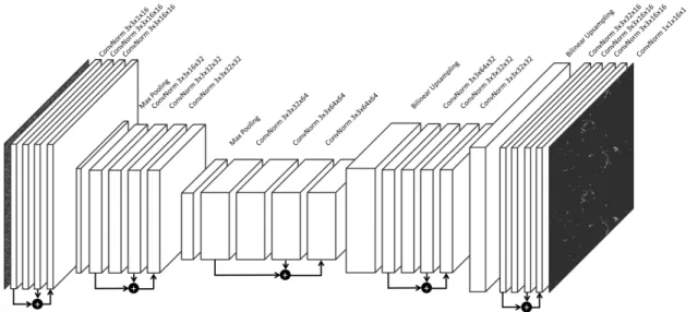
the top and the detailed layer configuration is delineated at the bottom. 22 2.3 Illustration of unfolding RNN over observations x. . . 23 2.4 LSTM architecture . . . 24 2.5 GRU architecture . . . 25 2.6 Generic hourglass-shaped neural network architecture. The original

image is the input on the left and the output is generated on the right. Arrows pointing downwards denote pooling and arrows pointing upwards denote unpooling. The convolutional layer blocks perform feature extraction or fusion. The dotted line separates the contracting path and the expanding path of the network. More recently, archi-tectures incorporate long skip connections between contracting and expanding path. . . 28 3.1 Deep neural network architecture of DetNet. The specific layer

config-uration is given above each layer. . . 35 3.2 Deep neural network architecture of DPT. . . 36 3.3 Workflow for grading breast cancer WSIs based on mitotic cell counts. 41 3.4 Example image demonstrating the artefact detection mechanism. . . . 42 3.5 Example demonstrating the attention mechanism. . . 42 3.6 Deep Consensus Network architecture. A FPN is used for multi-scale

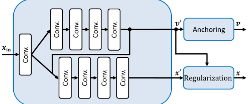
feature extraction, CPNs for predicting object centroids, consensus voting for aggregation of predictions, and centroid-based NMS for eliminating conflicting proposals. . . 45 3.7 Anchors used as voting priors. . . 46 3.8 Centroid Proposal Network (CPN) and subsequent anchor and

regular-ization steps. The offset vectorsv0predicted by the CPN are combined with their corresponding anchors and the predicted confidence scores P(v0) are regularized using the magnitude of the offset vectors v0. . . 47

(13)

List of Figures

3.9 Computation time for the proposed centroid-based NMS vs. a vanilla NMS. The standard deviation over 10 runs is shown by error bars. . . 50 3.10 Gradient of CE, LDice, LNMI, and Lcls calculated on samples Xi, Yi

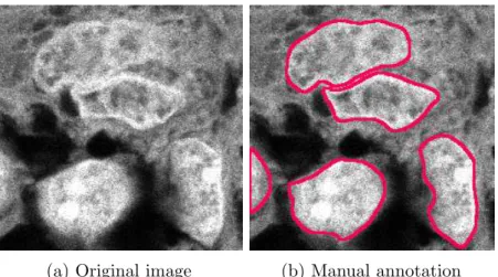
within batches X,Y with class balance of 0.01, 0.50, and 0.99. The curve wherex is equal toy is marked in black. . . 58 4.1 DAPI channel of original tissue image of glioblastoma cells and ground

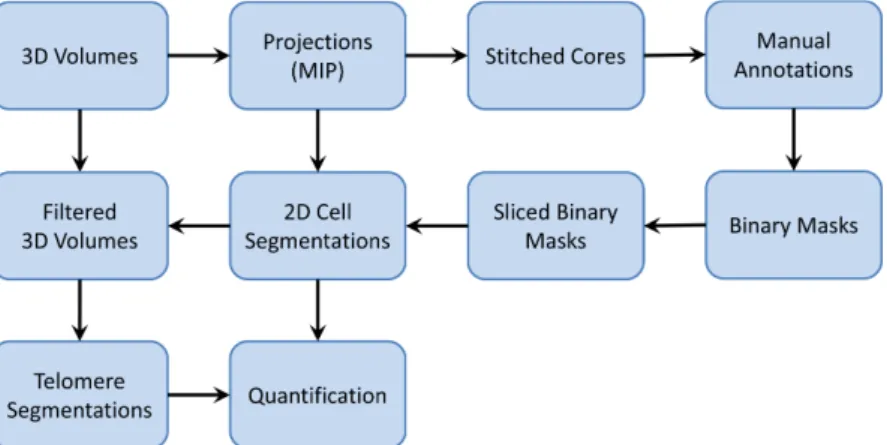
truth annotation. . . 62 4.2 Deep neural network architecture of ASPP-Net . . . 62 4.3 Workflow for telomere quantification in glioblastoma and prostate

tissue images. . . 63 4.4 GRUU-Net architecture. Red circles with an arrow pointing

up-ward/downward denote unpooling/pooling. At each scale Full-Resolution Dense Units (FRDUs) extract features, which are aggregated by a gated recurrent unit (GRU). . . 66 4.5 Full-Resolution Dense Unit (FRDU) . . . 68 4.6 Scheme for distributed data augmentation and training. Blue boxes are

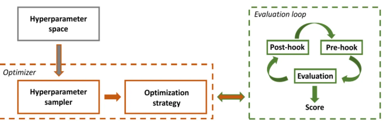
CPU management processes and green boxes CPU compute threads. Grey boxes represent pre-processed files and dotted lines indicate file access. Red boxes represent GPU computations. Dashed rectangles denote compute nodes connected by threads creation (solid lines) outlining the hierarchy tree of thread forks. . . 71 5.1 Schematic representation of HyperHyper software architecture with

modular structure. . . 77 6.1 Different approaches for transfer learning. . . 80 6.2 Overall workflow of the proposed method. . . 82 7.1 Detection results for HCV live cell microscopy data. a) Ground truth

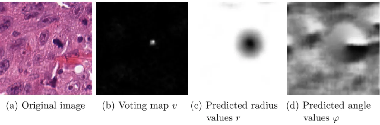
particles indicated by red circles. The yellow box represents the training data. Detection results for b) SEF, c) H-Dome, and d) DetNet. 88 7.2 Example region of an original image with corresponding voting result

and predictions of the radius and angle. . . 89 7.3 CE (green), WCE (blue), NFL (magenta),LDice(yellow),LMCC(black),

andLcls (red) for prediction/ground truth sample pairs from the nor-malized confusion matrix. The predictions were augmented with exponential noise. This scheme was repeated 1000 times. The figure shows the mean as line and the standard deviation as colored area. For each subplot two entries of the normalized confusion matrix were changed and the other two were fixed (set to 0.25). . . 92 7.4 Example images showing image sections of all employed scenarios from

the Particle Tracking Challenge dataset. . . 93 7.5 Example detection results of the Deep Consensus Network for sections

from the Particle Tracking Challenge dataset. . . 93 7.6 Example images showing hard to distinguish mitotic and non-mitotic

(14)

List of Figures

7.7 Example detection result of Deep Consensus Network for a section of 5657×3880 pixels from the TUPAC16 challenge dataset. . . 97 7.8 Examples of tissue microscopy images of glioblastoma cells with

dif-ferent challenges for image analysis. . . 100 7.9 Segmentation results of different methods for an example of a tissue

microscopy image of glioblastoma cells. . . 101 7.10 Segmentation results of GRUU-Net, U-Net, and corresponding ground

truth annotations for two example images of tissue microscopy images of glioblastoma cells (top, bottom) . . . 104 7.11 (a) Original and normalized focal loss for the validation set during

training. The values were normalized with respect to the maximum value. (b) Dice coefficient for the validation set during training for original and normalized focal loss. . . 106 7.12 (a) Original fluorescence microscopy image of rat mesenchymal stem

cells (Fluo-C2DL-MSC) from the Cell Tracking Challenge, (b) corre-sponding ground truth, and (c)-(k) segmentation results of GRUU-Net for different iterations. . . 107 7.13 Sample images showing the variability of image data in the Cell

Tracking Challenge datasets (partially contrast-enhanced for better visibility). . . 108 7.14 Examples of prostate tissue images showing various challenges for

image analysis. a) Strong background noise. b) Strong shape variation. c) Strong intensity variation. d) Low contrast. . . 115 7.15 Convergence of different optimizers as a function of the number of

iterations. a) K-means clustering pipeline. b) U-Net pipeline. . . 116 7.16 Comparison of segmentation results for both pipelines with different

optimizers. a) Original image. b) Original image with ground truth annotations by an expert. c) K-means clustering pipeline with CMA-ES. d) K-means clustering pipeline with SMAC-RF. e) U-Net pipeline with CMA-ES. f) U-Net pipeline with SMAC-XGBoost. . . 117 7.17 Detection results for HCV live cell microscopy data with different

hyperparameter optimizations. a) Ground truth annotated by an expert. b) Experiment 2 using Grid Search c) Experiment 2 using SMAC-RF. d) Experiment 3 using Grid Search. . . 119 7.18 Convergence of different optimizers as a function of the number of

iterations. . . 119 7.19 Loss surface of experiment 2 for 2D hyperparameter space (c and

σLoG). a) The hyperparameter space was sampled with Grid Search and the global optimum is marked with a blue star. b) Same as in a), but with optimization trails of Random (green) and SMAC-RF (blue). For both trails, the dot is the starting point and the star shows the found optimal solution. Both trails represent the best evaluations per optimization step over time. . . 120 7.20 HCV fluorescence microscopy data. a) Original image. b)

Pre-processed image with optimal σGauss obtained by Grid Search. . . 121 xiv

(15)

List of Figures

7.21 Infimum projections of the loss surface from experiment 3 for the 3D hyperparameter space (c, σLoG, andσGauss) sampled with Grid Search. The global optimum is marked with a blue star. . . 122 7.22 Example tissue microscopy image of glioblastoma cells, ground truth,

and segmentation results of different methods. . . 124 7.23 Examples of regions of interest automatically selected from a WSI. . . 125 7.24 Images (512×512 pixels) from different data sources mapped to Data 1.126 8.1 Galaxy Image Analysis workflow for cell segmentation and counting. . 133 8.2 GIEs for explorative data analysis. . . 134 8.3 GIE for server-side image rendering and visualization based on ParaView.134 8.4 GIE for WSI visualization based on OpenSlides Deep Zoom

imple-mentation. . . 135 8.5 Galaxy Image Analysis workflow for foci analysis. . . 138 8.6 User interface for interactive merging foci segmentation masks within

the foci analysis workflow. . . 138 8.7 Example original and annotated image showing infected cells. . . 139 8.8 Galaxy user interface for configuring neuron quantification tools. . . . 139 8.9 Example H&E-stained and MALDI WSI and TMA images along with

ROIs annotated on the H&E-stained images. . . 141 8.10 MALDI and HE image registration workflow. . . 141 8.11 Example result for the registration of an H&E image with a MALDI

(16)

List of Tables

1.1 Overview of microscopy techniques considered in this thesis . . . 6 3.1 Deep Residual Hough Voting architecture . . . 38 4.1 GRUU-Net layer configuration. The superscripts denote the filter size

for the convolutions and the number of layers k in the Dense blocks of the FRDU. The subscripts represent the number of output feature maps. . . 69 5.1 Comparison of different hyperparameter optimization frameworks. . . 76 5.2 Investigated optimizers and corresponding sampling and optimization

strategies . . . 78 7.1 Performance for the Particle Tracking Challenge data (mean ±

stan-dard deviation). . . 87 7.2 Impact of sigmoid shift a (vesicle data, SNR=1). . . 87 7.3 Performance for HCV live cell microscopy data. . . 88 7.4 Performance of the proposed approach and comparison with top-3

methods from AMIDA13. . . 90 7.5 Results for the methods in the TUPAC16 challenge that only used

the provided training dataset. . . 91 7.6 Standard deviation of normalized performance metrics when changing

two entries of the confusion matrix (cf. Figure 7.3). . . 92 7.7 Performance of different detection methods for the Particle Tracking

Challenge receptor data. . . 94 7.8 Performance of different detection methods for the Particle Tracking

Challenge vesicle data. . . 94 7.9 Performance of different detection methods for the Particle Tracking

Challenge microtubule data. . . 95 7.10 Performance of the proposed approach and comparison with previously

proposed methods and top performer from TUPAC16. . . 97 7.11 Pixel-based performance metrics for different segmentation methods.

The values are mean values over 20 images. The best results are highlighted in bold. * _{Two different parameter settings used. . . 102} 7.12 Object-based performance metrics for different segmentation methods.

The values are mean values over 20 images. The best results are highlighted in bold. * _{Two different parameter settings used. . . 102} 7.13 Ablation study of the proposed data augmentation method for the

glioblastoma dataset using the U-Net and the proposed GRUU-Net . 103 7.14 Comparison of methods for the glioblastoma dataset . . . 105 7.15 Results for the real 2D datasets of the Cell Tracking Challenge . . . . 109 7.16 Results for the real 3D datasets of the Cell Tracking Challenge . . . . 112

(17)

List of Tables

7.17 Mean average precision of instance segmentation methods using a FPN backbone on the 2018 Data Science Bowl challenge dataset. . . 114 7.18 Results for the K-means clustering and U-Net pipeline with different

optimizers. The table shows the improvement ∆Dice (mean± std.) after the warm-up phase and the absolute Dice value (mean± std.). The best results are highlighted in bold. . . 116 7.19 Results for the HCV protein detection pipeline with different

optimiz-ers. The table shows the improvement ∆F1 (mean± std.) after the warm-up phase and the absolute F1 score (mean ± std.). The best results are highlighted in bold. . . 118 7.20 Results for the two HCV protein detection pipelines (experiment 2

and 3) with Grid Search. The table shows the absolute F1 score. The best result is highlighted in bold. . . 120 7.21 Results of PCA for the whole loss surface data. The table provides the

eigenvectors and eigenvalues of the four principal components (PC) together with the ratio between the cumulative variance and the total variance in [%]. . . 121 7.22 Performance of different segmentation methods. Bold and underline

highlights the best result, and bold indicates the second best result. . 124 7.23 Results for state-of-the-art data augmentation and for domain

adap-tation. . . 126 8.1 Comparison of KNIME and Galaxy characteristics. . . 131 8.2 Comparison of genome data and image data. . . 133 8.3 SUS questionnaire usability studies for ImageJ, KNIME, and Galaxy. 136 8.4 SUS questionnaire usability scores only for participants trained in the

use of the respective software. . . 137 8.5 Quantitative evaluation of the neuron detection approach. . . 140 8.6 Quantitative evaluation of the automatic H&E and MALDI

(18)

Nomenclature

Mathematical symbols frequently used in this thesis.

Hadamard product

∗ Convolution operator

vec(A) Vectorization of a matrix A

L Loss function

x Input tensor of layer

y Output tensor of layer

X Prediction vector

Y Ground truth vector

W Weight tensor of layer t Iteration/time

i Layer/Neuron index b Batch size

w×h Feature map width and height p Number of input feature maps q Number of output feature maps k Window size of convolution kernel

(19)

Publications

Major parts of this thesis have been published in reviewed journals and peer-reviewed conference proceedings.

Peer-Reviewed Journal Articles

T. Wollmann and K. Rohr, “Deep Consensus Network: Aggregating predictions to improve object detection in microscopy images,” under review, 2020

T. Wollmann, M. Gunkel, I. Chung, H. Erfle, and K. Rohr, “GRUU-Net: Integrated convolutional and gated recurrent neural network for cell segmentation,”Med. Image Anal., vol. 56, pp. 68–79, 2019

C. Ritter,T. Wollmann, P. Bernhard, M. Gunkel, D. M. Braun, J.-Y. Lee, J. Mein-ers, R. Simon, G. Sauter, H. Erfle, K. Rippe, R. Bartenschlager, and K. Rohr, “Hyperparameter optimization for image analysis: Application to prostate tissue

images and live cell data of virus-infected cells,” Int. J. Comput. Assist. Radiol. Surg., vol. 14, no. 11, pp. 1847–1857, 2019

M. Veta, Y. J. Heng, N. Stathonikos, B. E. Bejnordi, F. Beca, T. Wollmann, K. Rohr, M. A. Shah, D. Wang, M. Rousson, et al., “Predicting breast tumor proliferation from whole-slide images: The TUPAC16 challenge,”Med. Image Anal., vol. 54, pp. 111–121, 2019

M. C. F¨oll, L. Moritz, T. Wollmann, M. N. Stillger, N. Vockert, M. Werner, P. Bronsert, K. Rohr, B. A. Gr¨uning, and O. Schilling, “Accessible and reproducible mass spectrometry imaging data analysis in Galaxy,” GigaScience, vol. 8, no. 12, p. giz143, 2019

B. Grüning, R. Dale, A. Sjödin, B. A. Chapman, J. Rowe, C. H. Tomkins-Tinch, R. Valieris, A. Caprez, B. Batut, M. Haudgaard, T. Cokelaer, K. A. Beauchamp, B. S. Pedersen, Y. Hoogstrate, D. Ryan, A. Bretaudeau, G. L. Corguillé, C. Brueffer, D. Yusuf, S. Luna-Valero, R. Kirchner, K. Brinda, M. Raden, T. Wollmann, J. Köster,et al., “Bioconda: A sustainable and comprehensive software distribution for the life sciences,” Nat. Methods, vol. 15, pp. 475—-476, 2018

T. Wollmann, H. Erfle, R. Eils, K. Rohr, and M. Gunkel, “Workflows for microscopy image analysis and cellular phenotyping,”J. Biotechnol, vol. 261, pp. 70–75, 2017

(20)

Publications

Peer-Reviewed Conference Proceedings

C. Ritter,T. Wollmann, J.-Y. Lee, R. Bartenschlager, and K. Rohr, “Deep learning particle detection for probabilistic tracking in fluorescence microscopy,” in Proc. ISBI, IEEE, 2020

T. Wollmann, C. Ritter, J.-N. Dohrke, J.-Y. Lee, R. Bartenschlager, and K. Rohr, “DetNet: Deep neural network for particle detection in microscopy images,” in Proc.

ISBI, pp. 517–520, IEEE, 2019

T. Wollmann, P. Bernhard, M. Gunkel, D. M. Braun, J. Meiners, R. Simon, G. Sauter, H. Erfle, K. Rippe, and K. Rohr, “Black-box hyperparameter optimization for nuclei segmentation in prostate tissue images,” in Proc. BVM, pp. 345–350, Springer, 2019

T. Wollmann, C. S. Eijkman, and K. Rohr, “Adversarial domain adaptation to improve automatic breast cancer grading in lymph nodes,” inProc. ISBI, pp. 582–585, IEEE, 2018

T. Wollmann, J. Ivanova, and K. Rohr, “Multi-channel deep transfer learning for nuclei segmentation in glioblastoma cell tissue images,” in Proc. BVM, pp. 316–321, Springer, 2018

R. Spilger, T. Wollmann, Y. Qiang, A. Imle, J.-Y. Lee, B. M¨uller, O. T. Fackler, R. Bartenschlager, and K. Rohr, “Deep Particle Tracker: Automatic tracking of particles in fluorescence microscopy images Using deep learning,” in Proc. MICCAI Workshop DLMIA, pp. 128–136, Springer, 2018

D. Baltissen, T. Wollmann, M. Gunkel, I. Chung, H. Erfle, K. Rippe, and K. Rohr, “Comparison of segmentation methods for tissue microscopy images of glioblastoma

cells,” in Proc. ISBI, pp. 396–399, IEEE, 2018

T. Wollmann and K. Rohr, “Deep residual Hough voting for cell detection in histopathology images,” in Proc. ISBI, pp. 341–344, IEEE, 2017

T. Wollmann and K. Rohr, “Automatic grading of breast cancer whole-slide histopathology images,” in Proc. BVM, pp. 249–253, Springer, 2017

(21)

1 Introduction

1.1 Motivation

In biomedical research, information about physiological processes is often required to verify research hypotheses [18]. Microscopy imaging is one of the most important techniques to extract such information [19]. Since manual analysis is generally too slow, labour-intensive, and prone to errors, automatic analysis is required to process the constantly increasing amount of microscopy image data.

The complexity of acquired microscopy images poses many challenges for image analysis algorithms. In recent years, deep learning improved the state-of-the-art in many computer vision tasks [20, 21, 22]. Especially, advances in deep learning methods for object detection [23, 24, 25], semantic segmentation [26, 27, 28], and classification of images [1, 29, 30] lead to improved results. Object detection and segmentation are frequent tasks to analyse high-content microscopy images, and deep learning has been used for such kind of images (e.g., [31, 32]). However, most of the existing deep learning methods have been developed for images of natural scenes. Biomedical images and particularly microscopy images raise additional domain-specific challenges compared to images of natural scenes (e.g., small objects, low SNR). The images vary significantly due to the experimental setup, imaging workflows, and imaging modalities. In addition, large annotated training datasets like COCO [33] or ImageNet [34] for natural images are not available for biomedical data. Biomedical image datasets often suffer from low annotation standardization and significant label noise. Moreover, usage of cutting-edge computer vision methods and especially methods based on deep learning is currently quite complex. Utilization of high-performance computing (HPC) and cloud compute infrastructure is too cumbersome for most biomedical researchers.

This thesis addresses different challenges that are important for successfully using deep learning in high-content microscopy image analysis. The main topics of this thesis are outlined in Figure 1.1. The different chapters cope withchallenges posed by microscopy datasets, introduce novel deep learning methods, and consider the deployment of image analysis workflows. Noveldeep learning methods are proposed for main tasks of microscopy image analysis, namely detection and segmentation. In addition, automatic optimization of the hyperparameters of software pipelines, transfer learning for reusing trained networks, and data augmentation to cope with the lack of training data are investigated to address dataset-specific challenges. Furthermore, aconcept for web-based image analysis and a system for deployment of

(22)

1 Introduction

Figure 1.1: Main topics of this thesis.

image analysis software in a research environment are presented.

1.1.1 Biomedical Microscopy Imaging

In medicine and biology, investigated structures like tissue microstructures, cells, viruses, or bacteria are too small to be seen with the naked eye. Microscopy techniques can provide magnified visual or photographic images of these structures [19]. Microscopes leverage light (optical microscope), electrons (electron microscope), or a scanning probe (scanning probe microscope) for capturing structures. This thesis focuses on optical microscopy modalities and considers an application of mass spectrometry imaging combined with optical microscopy. In the following, an overview of these modalities is given.

An optical microscope typically consists of an object slide containing the structures of interest, a system of lenses for magnification and filtering, which creates the image in the intermediate plane and is observable in the eyepiece or digitalized using an image sensor, and, depending on the technique, an illumination module [19]. An object is in focus when the light rays originating from the object specimen converge in the eyepiece or image sensor. In this thesis, datasets from translumination-based (bright-field, phase-contrast, differential interference contrast) and fluorescence-based (widefield, confocal, spinning disk) microscopes are analysed. Translumination microscopy can image tissue by transmitting light through the object slide [19]. In bright-field microscopy, the object slide is illuminated with white light and the absorption of the light creates contrast in the resulting image [19]. Stainings can be used to increase light absorption of certain structures, which accentuate them in the image. Unstained tissue is hardly visible in bright-field microscopes as it is mostly translucent. Phase-contrast microscopy can image translucent objects using phase shifts in light passing

(23)

1 Introduction

through the object of interest. A phase-shift ring is used to shift the phase of the light by 90◦ or -90◦ that passed the slide. After filtering, the background light and the light scattered by the object overlay and the resulting constructive interference creates visual contrast. Differential interference contrast (DIC) microscopy is an alternative method to image translucent objects by interferometry. The light is first polarized and then separated into two rays, which are focused on the sample. After passing the sample, the rays are overlaid using a prism and contrast is created by constructive interference. Fluorescence microscopy can image fluorophore stained tissue which emits light when being illuminated [19]. The excitation spectrum is the required light which has to be emitted by the fluorescent light source to stimulate the fluorophore so that it emits light in its characteristic emission spectrum. There exist several fluorescence microscopy techniques like widefield, laser scanning, and spinning disk microscopy. The differences of the pattern of illumination is illustrated in Figure 1.2. In widefield microscopy, the whole slide is illuminated which then excites fluorophores [19]. The main disadvantage of widefield microscopy is that light emitted from the specimen out-of-focus interferes with the light emitted within focus, which reduces the maximum resolution in addition to the thickness of the specimen. Confocal microscopy uses the pinhole principle to only detect light from the image plane in focus. Confocal laser scanning microscopy (CLSM) uses a laser for illumination, which scans the slide in a raster pattern and uses a photomultiplier tube to detect the signal for each spot. Compared to widefield microscopy, single coordinates in 3D can be imaged. CLSM is comparably slow, since each coordinate has to be imaged sequentially. In spinning disk confocal laser microscopy (SDCLM), multiple coordinates are illuminated simultaneously by leveraging multiplexing. Multiple pinholes are arranged on a mechanically spinning Nipkow disk in a specific pattern. A dichroic mirror is used to separate scattered/reflected light and laser light from the optics. Depending on the design, a second or the same Nipkow disk is used as light shade for each corresponding pinhole of the first Nipkow disk transit. In SDCLM, camera detectors are used instead of a photomultiplier tube. They have the advantage of a higher quantum efficiency. Therefore, images with a higher signal to noise ratio can be obtained compared to CLSM. Multiple operating modes can be combined in a single device like the microscope shown in Figure 1.3. A drawback of fluorescence microscopy is that fluorescent stains are phototoxic, invasive, and bleach

(a) Widefield (b) Laser scanning (c) Spinning disk

(24)

1 Introduction

Figure 1.3: Optical table with Nikon Eclipse Ti2 microscope, which supports phase-contrast, DIC, CLSM, and SDCLM operating modes.

when being illuminated, which makes them more challenging for live cell imaging than other techniques [19].

Many microscopy techniques benefit from or require stained specimen to enhance contrast of structures of interest. Essential stains and dyes in biology and medicine are hematoxylin and eosin stain (H&E) and 4’,6-diamidino-2-phenylindole (DAPI) [19]. H&E staining is usually used for bright-field microscopy in histology [19]. Hematoxylin binds to basophilic substances and appears as dark blue or violet in the image. Deoxyribonucleic acid (DNA) and ribonucleic acid (RNA) are negatively charged and therefore acidic, which makes them basophilic. The chromosomes consisting of DNA are usually located in the cell nucleus, and RNA is highly concentrated in the ribosomes of the rough endoplasmic reticulum (Figure 1.4). The different cell states like cell division (mitotic phase), programmed cell death (apoptosis), or premature cell death (necrosis) manifest in different chromosome appearance. As opposed to hematoxylin, eosin binds to acidophilic substances and is seen in red or pink in the image. Amino acids and proteins that are amino acid complexes are basic, as the molecules are positively charged due to their arginine and lysine residues. Amino acids and proteins are highly concentrated in structures

Figure 1.4: Eukaryotic cell in a simplified cutaway drawing

(25)

1 Introduction

like the cytoplasm and cell organelles (e.g., mitochondria, erythrocytes, collagen, extracellular fibers). The Golgi apparatus, myelin, or adipocytes are hydrophobic structures and remain clear when using H&E staining as the stain is water-based. Immunostainings are used to detect specific proteins by exploiting the antibody mechanism to target the proteins of interest. DAPI is an essential stain in fluorescence microscopy [19]. It mainly binds to the regions rich in adenine-thymine in the DNA, dyeing the nucleus. DAPI also binds to RNA with a different emission wavelength. A main advantage of DAPI is that it can be combined with other popular dyes like GFP or CY3. However, cross-talk and bleed-through can occur when multiple stains are used. The cross-talk effect describes that dyes with overlapping excitation spectrum are illuminated at the same time. Bleed-through describes the effect that the emission spectra of two stains have an overlap so that the filters and detectors are not able to separate the signals. More specialized fluorescence stainings (e.g., GFP, CY3, FAM, Alexa Fluor) can be modified by using techniques like fluorescence in situ hybridization (FISH) to bind to specific structures (e.g., centromeres, telomeres, target genes).

A stain-free, but destructive microscopy method is spatially-resolved mass spec-trometry [35]. Matrix-assisted laser desorption/ionization (MALDI) is an ionization technique where a matrix material is added to the sample (Figure 1.5b) [36]. A laser is used to ionize the sample and to excavate macro molecules. These ionized molecules are usually proteins that can be detected using by their time of flight (ToF) in a mass spectrometer (Figure 1.5a). When applying the laser grid-wise on a slide, spatially-resolved mass spectra can be obtained. MALDI-ToF can be applied to an already stained sample and can therefore be combined with optical microscopy [36].

The modalities, stainings, and dyes considered in this thesis are summarized in Table 1.1.

(a) Matrix sprayer (b) MALDI-ToF mass spectrometry

(26)

1 Introduction

Table 1.1: Overview of microscopy techniques considered in this thesis Microscopy Principle Contrast Technique Modality Staining & Dye

Optical

Translumination

Bright-field H&E, Immuno Phase-contrast -DIC Fluorescence Widefield DAPI, GFP, CY3, FAM, Alexa Fluor CLSM SDCLM

Mass spectrometry Desorption/Ionization MALDI

-1.1.2 Biomedical Microscopy Image Analysis

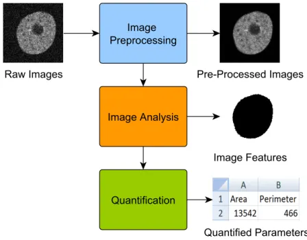
In a biological or medical research, where complex image data like high-content or high-throughput microscopy images are acquired using the imaging techniques described above, manual analysis is often not feasible. Automated image analysis can help coping with the data. A meta image analysis workflow of images in biology and medicine is illustrated in Figure 1.6 and consists of three main steps.

First, the images are pre-processed to improve the image quality and enhance meaningful content. Methods for pre-processing images are mostly based on filters (e.g., median rank filter, Gabor filter, histogram equalization). These filters can be

applied within a sliding window or the whole image.

Second, specific features of interest are extracted usingimage analysis methods like object detection, segmentation, image classification, image registration, and object

Figure 1.6: Meta image analysis workflow with an example of cellular phenotyping

(27)

1 Introduction

tracking. Object detection can be performed by using local feature descriptors (e.g., SIFT, ORB) [37], which can be combined with a classifier (e.g., Logistic regression, Random Forrest, Support Vector Machine) [38]. Segmentation methods can be categorized by their definition of image segments. This includes methods without shape guidance based on histogram thresholding (e.g, Otsu’s method) or clustering (e.g., K-Means, Mean-Shift, Hierarchical clustering) and with shape guidance using image regions (e.g., Region Growing) or model energy (e.g., Markov Random Fields, Level sets) [39]. Image classification can be conducted using global feature descriptors (e.g., Haralick features) [37] in combination with a classifier. Registration of images can be performed based on image intensity or features and a similarity measure (e.g., cross-correlation, mutual information) [39]. Object tracking can be based on object detection (tracking-by-detection). The detections can be linked into tracks (e.g., using a Kalman filter) [40]. Most traditional image analysis methods include hand-crafted features. Development of good feature extractors requires deep domain knowledge. Deep learning can be used to learn feature extractors without the need of explicitly modelling domain knowledge. These feature extractors can be used in various image analysis methods. Therefore, feature extraction and classification can be performed jointly by using deep learning. State-of-the-art in image analysis methods for detection and segmentation based on deep learning are described in Chapter 2.

Finally, the extracted features (e.g., cell count, cell elongation, mean stain intensity, tissue texture statistics, particle velocity) are quantified. Often, rule-based filtering is used for the quantified data to account for sup-optimal image analysis results. The resultingreadout is used to reach a medical or biological conclusion along with the hypothesis.

Software can help biologists to use existing image analysis methods on their image data [41]. If no appropriate method for certain data is available or the required image analysis pipeline is too complicated, image analysis researcher are consulted. In these research projects, image analysis researchers and biologists collaborate closely. In Figure 1.7, a typical workflow of such a project is sketched. The medical or biological cooperation partner produces image data which is handed to the image analysis researcher. The image analysis researcher develops a method and a corresponding software and uses it to generate the desiredreadout (e.g., cell counts, cell phenotypes,

(28)

1 Introduction

particle behavior). The readout is given to the cooperation partner to answer their biological or medical research hypothesis. Image acquisition and image analysis methods are continuously improved during the project. However, often the image analysis researcher has to run the software for a new dataset even if no changes to the software have been introduced, since most of the experimental image analysis pipelines are too cumbersome to use and therefore cannot be run by the biologist.

1.2 Contributions

This thesis proposes methods for easing frequent problems with biomedical microscopy datasets, improves deep learning models for biomedical computer vision, and presents a concept for deployment of cutting-edge algorithms in biomedical research projects. More specifically, the main contributions of this thesis are:

DetNet – Deep Neural Network for Particle Detection: A new method for particle detection in microscopy images is proposed which uses deep learning and is based on a domain-adapted Deconvolution Network. Compared to standard deep neural network architectures, the number of parameters is significantly reduced. The method achieved better detection and localization results than previous methods.

Deep Residual Hough Voting for Mitotic Cell Detection in Histopathol-ogy Images: A new method for mitotic cell detection in histopathology images is proposed which is based on a Deep Residual Network architecture combined with Hough voting. A voting layer for neural networks is proposed. Also, a novel loss function is introduced, which exploits polar coordinates and is invariant to the absolute magnitude of the voting error. The network is learned from scratch using cell centroids. In addition, a new method for grading whole-slide histology images of invasive breast carcinoma is proposed which is based on mitotic cell detection by a Deep Residual Network. The method combines a threshold-based attention mechanism and a deep neural network for mitotic cell detection and grading.

Deep Consensus Network for Particle and Cell Detection: A new deep neural network named Deep Consensus Network (ConsensusNet) for particle and cell detection in microscopy images based on object centroids is introduced. The network is trainable end-to-end and comprises a Feature Pyramid Network-based feature extractor, a Centroid Proposal Network, and a layer for ensembling detec-tion hypotheses over all image scales and anchors. Also, an anchor regularizadetec-tion scheme that favours prior anchors over regressed locations is suggested. In addition, an improved algorithm for Non-Maximum Suppression which significantly reduces the algorithmic complexity, is introduced. The method was applied to challenging data from the TUPAC16 mitosis detection challenge and the Particle Tracking

(29)

1 Introduction

challenge and generally yielded better results than DetNet, Deep Residual Hough Voting, and previous methods.

Loss Function for Strong Class Imbalance in Object Detection: For the Deep Consensus Network, a novel loss function based on Normalized Mutual Information is proposed. The loss can cope with strong class imbalance and is derived within a Bayesian framework.

ASPP-Net for Cell Segmentation: A deep learning method leveraging atrous spatial pyramid pooling (ASPP) for cell segmentation is introduced. The ASPP increases the receptive field of the network to capture rich semantic information. The method is used in a workflow for large scale quantification of telomere length and PITX1 expression per cell.

GRUU-Net – Integrated Convolutional and Gated Recurrent Neural Network for Cell Segmentation: The dominant paradigm in segmentation is using convolutional neural networks, less common are recurrent neural networks. A new deep learning method for cell segmentation is proposed which integrates convolutional neural networks and gated recurrent neural networks over multiple image scales to exploit the strength of both types of networks. The method was applied to images of cells from various modalities and yielded better results than previous methods.

Loss Function to Cope with Difficult Samples in Image Segmentation:

To increase the robustness of the training and improve segmentation, a novel focal loss function for GRUU-Net is introduced. A distributed scheme for optimized training of the integrated neural network is presented as well.

Hyperparameter Optimization: A framework for zero-order black-box hy-perparameter optimization called HyperHyper is presented which has a novel modular architecture that separates hyperparameter sampling and optimization. A visualization of the loss function based on infimum projection to obtain further insights into the optimization problem is also introduced.

Multi-Channel Deep Transfer Learning: Two different approaches for trans-fer learning using fluorescence images of glioblastoma cell tissue with a diftrans-ferent number of color channels are presented. The approaches exploit the similarity of source image channels and target image channels and are based on the ASPP-Net.

Unsupervised Domain Adaption for End-to-End Grading of Whole-Slide Images: A novel deep learning method for domain adaption and classifica-tion of whole-slide images and patient level breast cancer grading is described. The proposed method is based on domain adaptation using a Cycle-Consistent Gener-ative Adversarial Network (CycleGAN) in conjunction with a densely connected deep neural network.

(30)

1 Introduction

Web-Based Microscopy Image Analysis: The platform Galaxy Image Anal-ysis for automated microscopy image analAnal-ysis and cellular phenotyping within the Galaxy platform is introduced. Workflows for cell segmentation in cell culture images, particle detection in mice brain tissue data, and MALDI-/H&E image registration based on Galaxy Image Analysis are presented.

1.3 Organization of the Thesis

The thesis describes novel deep learning methods for object detection and segmen-tation. In Chapter 2, fundamentals of deep learning and previous work on object detection and segmentation are outlined. Chapter 3 introduces novel deep learning methods for detection of particles and cells. In Chapter 4, deep learning methods for segmentation of cells and an application to telomere quantification in tissue images are proposed. Chapter 5 introduces a framework for hyperparameter optimization of software pipelines in microscopy image analysis. Chapter 6 describes new methods for transfer learning for microscopy images. The evaluation of the proposed deep learning methods is presented in Chapter 7. A web-based framework for microscopy image analysis named Galaxy Image Analysis and applications are described in Chapter 8.

An overview of the developed methods, their connections, and a classification into the categories Dataset Challenges, Deep Learning Methods, and Deployment described above (cf. Figure 1.1) is given in Figure 1.8.

Figure 1.8: Connectivity of sections and chapters in this thesis. The main topics of the thesis are highlighted in bold. Connections between sections indicate that the described methods build on each other.

(31)

2 Foundations and Previous Work

In this chapter, fundamental concepts that are essential for this thesis are introduced. In particular, foundations of deep learning for computer vision and recent develop-ments in the field of microscopy image analysis for detection and segmentation are reviewed. In this chapter, the fundamentals of deep learning for computer vision are presented. A review of state-of-the-art deep learning methods for object detection using bounding-boxes and centroids as well as semantic segmentation is conducted. Furthermore, applications and extensions of these methods for microscopy image analysis are elaborated on.

2.1 Deep Neural Networks for Computer Vision

Artificial Neural Networks (ANN)are a family of computation graphs loosely inspired by biological neural networks in animal brains. In an ANN, each layer of q neurons has the weight parametersW ∈_Rp×q _{and bias parameters} _b _∈

Rq, where p is the number of neuron activations of the previous layer. The activationyi ∈R of the i-th neuron is calculated by a weighted sum of the neuron activations of the previous layer x ∈ _Rp×1 _{using the weights} _w

i ∈ Rp×1 and the bias bi ∈ R followed by an activation function σ. Therefore, the activationyi ∈Rof the i-th neuron in a layer is as follows:

yi =σ((wi)|x+bi) (2.1) Theactivation function σcan be the identity function (linear function) or a non-linear function. Non-linear functions are required to capture the properties of complex data distributions. The orchestrated structure of multiple network components (e.g., layers, activations) is called network architecture. ANNs learn to perform a specific task by changing its parameters in the training phase using an optimization algorithm. The application of a trained network on data is called inference.

An ANN whose computation graph is directed and cycle-free is called feed-forward neural network (Figure 2.1). An early ANN is the Perceptron, which has one layer and the Heaviside step function as activation function [42]. If the network has at least one hidden layer, it is called multi-layer perceptron (MLP). More generally, an ANN with multiple consecutive hidden layers is called Deep Neural Network (DNN). The universal approximation theorem [43, 44] states that under mild assumptions (e.g., if σ is a non-constant, bounded, and a continuous function), a multi-layer feed-forward

(32)

Figure 2.1: Feed-forward neural network

neural network can approximate any continuous function in a compact set Ω ∈_Rn with an error bound which decreases with an increased number of neurons. Therefore, even a neural network with one hidden layer is an universal approximator. This raises the question how DNNs with a large number of parameters can be learned effectively in practice [45]. Recent theories state that an underlying hierarchical generation process exists in natural data, which can be decomposed into smaller problems by using the mutual information chain rule [46, 47]. Due to weight sharing within layers (see Section 2.1.1) and hierarchical composition of neurons, the underlying structure in data can be exploited to ease the network’s training [47]. Moreover, the stochastic algorithms for training neural networks favour local optima with good generalization properties [48, 49, 50, 51].

Model Training

A popular algorithm for training DNNs is stochastic gradient descent (SGD) in combination with backpropagation [52]. Firstly, the current output of the network for a batch of samples is calculated, which is called forward pass. Next, an error scoring function (loss) L ∈ _R is calculated based on the corresponding reference. In the backward pass, the i-th weight wi ∈R of a neuron is updated in each iteration t of the optimization using the SGD update rule with learning rate η ∈_R+_:

w_it←wt_i−1−η∇_wt−1

i L (2.2)

Assuming that L is a function of y and y is a function of x, the gradient of the loss ∇L for variables in lower layers can be back propagated using the chain rule of derivatives: ∂L ∂x = ∂L ∂y ∂y ∂x (2.3) 12

(33)

Therefore, unlike canonical gradient descent, SGD computes a parameter update for every batch instead for the whole dataset [53]. The incremental gradient descent of SGD introduces noise which helps escaping local minima and tends to more flatter minima than canonical gradient descent [48]. However, the surface of the loss, which depends on the data and the network’s architecture as visualized in [49], can be flat or spiky in some regions. To exploit the shape of the loss surface in the optimizer’s trajectory, an adaptive step size is advantageous. Therefore, the momentum of convergence is often used which also speeds up training and reduces oscillation of the loss. RMSprop is a popular extension to SGD, first presented by G. Hinton in a lecture of his Coursera class, which adaptively reduces the learning rate by exponentially decaying it by the squared derivative (∇_wt−1

i L) 2 _∈

R [54]. The influence of the momentum can be changed byβ ∈_R+_{, which is usually set to 0.9:}

wt_i ←w_it−1−η∇w t−1 i L p vt i + (2.4a) v_it←βv_it−1 + (1−β)(∇_wt−1 i L) 2 (2.4b) where is a small constant to avoid division by zero. Adam [55] is a more recent popular alternative to RMSprop, which in addition to the average of the squared derivative vt_i ∈_R also uses the average of the derivative mt_i ∈_R. The influence of mt_i andv_it can be changed by the parameters β1 ∈R[0,1] and β2 ∈R[0,1], which are usually set to 0.9 and 0.999 [55]:

wt_i ←w_it−1−η mˆ t i p ˆ vt i + (2.5a) ˆ mt_i = m t i 1−β1 (2.5b) ˆ vt_i = v t i 1−β2 (2.5c) mt_i ←β1mti−1+ (1−β1)∇w_it−1L (2.5d) v_it←β2vit−1 + (1−β2)(∇w_it−1L) 2 _(2.5e)

Reddi et al. [56] pointed out that the convergence of Adam can be harmed, since ˆvi does not necessarily increase when the learning rateηis constant or decreasing. They proposedAMSGrad, which only keeps track of the maximum squared derivative, to

(34)

ensure a decreasing learning rate over the training iterations: w_it←wt_i−1−η mˆ t i p ˆ vt i + (2.6a) ˆ mt_i = m t i 1−β1 (2.6b) ˆ v_it= max(v t i,vˆ t−1 i ) 1−β2 (2.6c) mt_i ←β1mti−1+ (1−β1)∇wt−_i 1L (2.6d) v_it←β2vit−1+ (1−β2)(∇_wt−1 i L) 2 _(2.6e)

Activation Functions

Several non-linear activation functions for neural networks are described in the literature (e.g., [57, 58, 59, 22]). Due to the universal approximation theorem, their expressiveness in a DNN is similar when using enough neurons [43, 44]. Their main difference in practice is their effect on the gradient. A major challenge in training deep neural networks is the vanishing gradient problem which was identified by Hochreiter in 1991 [60]. Due to weight updates performed using backpropagation, the gradient is proportional to the partial derivatives of the loss function. Poor architectural choices can lead to contracting gradients which are accumulated by the chain rule of derivatives. Bounded functions (e.g., Sigmoid, Tanh), for example, also have a bounded gradient which can exponentially decrease the gradient when used in every layer. A similar effect can be observed with exploding gradients where gradients accumulate, resulting in large weight updates. These two effects lead to unstable training or underfitted models. The Sigmoid function squashes the input x to [0,1]: Sigmoid(x) = ( ₁ 1+e−x , x > 0 ex ex₊₁ , x≤0 (2.7)

The output of the Sigmoid function is not zero-centred. This can be overcome with the hyperbolic tangent (Tanh), which squashes the input to [−1,1]. Due to the bound of Sigmoid and Tanh, the optimization can be harmed. In 2011, Glorot et al. [57] proposed the Rectified Linear Unit (ReLU) as an unbound alternative to

(35)

previous activation functions:

ReLU(x) = max(0, x) (2.8) When using ReLUs, the negative part of the neurons activation is not used. Therefore, neurons can be in a state where they become untrainable, since they have a derivative of zero. There are several variants of ReLUs that are designed to reduce this problem. The Leaky Rectified Linear Unit (LReLU) [58] makes use of a small negative component in its output by introducing a leakage parameter a= 0.2:

LReLU(x, a= const) =

(

x , x > 0

ax ,otherwise (2.9) The Parametric Rectified Linear Unit (PReLU) [59] is a generalization of LReLU, where the leakage parameter a∈_R can be trained along with the network:

PReLU(x, a) =

(

x , x >0

ax ,otherwise (2.10)

Network Weight Initialization

Weights in neural networks are initialized so that they keep a specific distribution over multiple layers, and additionally break symmetry so that each neuron can learn its distinct feature. Moreover, the activations should be zero-centered and have unit variance. State-of-the-art initialization schemes use values in the weight matrix W

sampled from a scaled random uniform or Gaussian distribution. To ensure similar distributions of activations in the network, Glorot and Bengio [57] proposed to use a variance Var(W) of the sampling distribution based on the number of neuronsnin in the previous and the number of neurons nout in the current layer:

Var(W) = 2 nin+nout

(2.11) When using activation functions like ReLU, half of the results are truncated. To overcome this, He et al. [59] proposed to only rely on the number of neurons in the previous layer: Var(W) = r 2 nin (2.12)

Model Regularization

State-of-the-art neural networks have millions of parameters and thus many degrees of freedom. They often have a learning capacity that exceeds the training dataset. In practice, the bias-variance tradeoff has to be considered to keep underfitting due

(36)

to high bias and overfitting due to high variance of the model in equilibrium [38]. By using regularization of the model, overfitting can be prevented. A common technique is to add `1 regularization: L=Lobj+λ N X i=1 |wi| (2.13)

or `2 regularization of the weight updates to the loss Lobj:

L=Lobj+λ N

X

i=1

(wi)2 (2.14)

where N is the number of elements of w. Regularization with `1 favours a sparse weight matrix and `2 favours a Gaussian distribution of the weights [38]. The influence of the regularization can be changed using the parameter λ∈_R. Another method of weight regularization using a norm is weight decay. Weight decay extends the SGD update rule (2.2) by adding a rescaling factor with a parameter λ to the weights: w_it←w_it−1 −η∇_wt−1 i L(w t−1 i )−ηλw t−1 i (2.15)

When using SGD, weight decay is similar to `2 regularization [61]. However, this does not hold for optimizers that use momentum. AdamW is an extension of Adam with weight decay [61]:

w_it←wt_i−1−η mˆ t i p ˆ vt i + −ηλwt_i−1 (2.16a) ˆ mt_i = m t i 1−β1 (2.16b) ˆ v_it= v t i 1−β2 (2.16c) mt_i ←β1mit−1 + (1−β1)(∇_wt−1 i L+λw t−1 i ) (2.16d) vt_i ←β2vit−1+ (1−β1)(∇w_it−1L+λw t−1 i ) (2.16e)

Another method to prevent overfitting is Dropout [62], which adds Gaussian or Bernoulli noise to the layer’s activations. Dropout can be interpreted as building random subgraphs within the neural network, which are robust to missing or wrong

(37)

inputs. Moreover, by adding noise to the activations, a Gaussian prior is put on the activations. In general, Dropout increases the training time, but improves the performance of the network. As the activation and weight distribution of neurons should not change throughout the network, the initial values of the parameters are initialized with a mean value of 0 and a unit variance of 1. However, in a forward pass, the distribution of activations can shift and scale, which also affects the weights as training progresses. This causes the weight distribution to degrade, slowing down training and triggering side-effects between layers. Batch normalization (BN) [63] is a simple, but effective technique which normalizes the activations in every layer and thus prevents the weight distributions from degradation. The shift β ∈_Rand scale γ ∈ _R of the activation distributions are learnable parameters of the architecture. The normalization is calculated for every batch withM samples using the mean value µb ∈_Rand the variance σ_b2 ∈_R+_{. Therefore, these estimates are noisy, and batch} normalization acts as a regularizer which often eliminates the need for Dropout [64]. During inference, the mean value µ∈_R and the variance σ2 _∈

R+ of the training dataset are used instead of the batch wise µb and σ2b:

BN(xi)≡γxˆi+β (2.17a) ˆ xi = xi−µb p σ2 b + (2.17b) µb = 1 M M X m=1 xm (2.17c) σ_b2 = 1 M M X m=1 (xm−µb)2 (2.17d)

In [65], the normalization is performed for each instance of a batch individually. Moreover,instance normalization is also applied during inference without learning any shift or scale parameters. In some use cases where dataset-wide shift and scale parameters are hard to learn, instance normalization can still simplify the learning process [65, 66]. A simple but effective method to improve generalization of the model is data augmentation. Data augmentation is the process of distorting data to enforce the network to learn invariance to these distortions. Common augmentations are flipping, rotation, adding Gaussian or Poisson noise, color shifting, histogram stretching, and elastic deformations [22]. Moreover, crops of a larger image can be sampled to specifically analyze more important regions [67]. Controlling the sampling of difficult cases and easy cases is referred to as hard negative mining. If the order of the samples is following a specific scheme, it is referred to as curriculum learning

(38)

[68]. Data augmentation can be performed offline on the training dataset, and online during training and at test time [69]. Test time augmentation is usually performed to exploit the invariance of the model and boost the performance by averaging the predictions of several augmentations of the same input. In data augmentation, it is important that the augmentation steps do not alter the semantics of the input. In addition, excessive augmentation can lead to too much smoothing and therefore underfitting. In general, a combination of regularization of the model and data augmentation usually works best in practice [70]. By using proper regularization, not only overfitting is avoided, but fast training of the model can be observed, which is referred to as superconvergence [71].

Loss Functions

For neural networks, several training objectives (loss functions) are used in computer vision. For classification tasks, thecross-entropy (CE) is commonly used, which mea-sures the average bits needed to encode an event drawn from probability distribution Q instead of the true distribution U, which is the sum of the entropy H of U and the Kullback-Leibler divergence DKL of U with respect to Qwhere Eis the expected value operator with respect to the distributionU [38, 22]:

CE(U, Q) = _EU[−log(Q)] = H(U) + DKL(U, Q) (2.18) In the discrete case, whereP(X)∈_RM _{are the predicted probabilities for the samples}

X = (X1, ..., XM) from Q and P(Y) ∈ RM the ground truth probabilities for the labels Y= (Y1, ..., YM) from U, we can define a CE-based loss LCE for M samples:

LCE(X,Y) = 1 M M X m=1 −P(Ym) log(P(Xm)) (2.19)

CE is defined for discrete events. Thus, classes are usually encoded in an indicator vector (one-hot vector). Therefore, the output is one for the index of one class and zero for all other classes. The output of the network can then be interpreted as a probability distribution across the classes. Classification can also be viewed regarding set theory. Based on the Dice coefficient, a smooth approximation can be minimized over the sets X and Y, where a small prevents a division by zero [72, 73]:

LDice(X,Y) =− 2PM m=1P(Xm) P(Ym) + PM m=1P(Xm) + PM m=1P(Ym) + (2.20)

The LDice loss has the advantage of implicitly weighting the loss using the class imbalance in the ground truth and the number of activations of the network. The Jaccard similarity coefficient and the Cosine similarity can also be used analogously as training objective. For regression tasks, usually a `p norm is used [22]. The `1 norm

(39)

k·k1, which is also known as taxicab metric, should not be favored for regression, since it has no always a unique solution and is therefore hard to optimize [38]. However, it can be used to enforce sparse results, which is important in regularization for tasks such as dictionary learning [74]. The `2 norm k·k2 is also known as Euclidean norm, has a unique solution, and is therefore the most common objective for regression. To further improve the stability of the training process, the squared `2 norm is used in the L`2 loss, which is also known as mean squared error (MSE):

L`2(v,v GT ) = 1 M M X m=1 kvm−vmGTk 2 2 (2.21)

where v∈_RM _{denotes the predicted values and} _vGT _∈

RM the ground truth values. The L`2 loss is prone to outliers since errors contribute quadratically to the total

error. Huber [75] proposed a piecewise defined loss LH with hyperparameter δ∈R, which is more robust than the L`2 loss:

LH(v,vGT) = 1 M M X m=1 (₁ 2(vm−v GT m )2 ,|vm−vmGT| ≤δ δ(|vm−vmGT| −12δ) ,otherwise (2.22)

Instead of explicitly formulating an objective, the loss function can also be learned along with the network [76] by usingadversarial training [77]. In adversarial training, a discriminator learns to classify a dataset, but engineered adversarial examples are added to fool the discriminator. It has been shown that neural networks are vulnerable to adversarial examples [78]. This method can be used by training a discriminator network to distinguish adversarial or original samples. A generator network is trained concurrently to generate adversarial samples from noise and is updated alternately to the discriminator network. This zero-sum game between the two networks forms an actor-critic model [79] known from reinforcement learning. The described combination of a generator and discriminator network known as Generative Adversarial Network (GAN) was introduced by Goodfellow et al. [76].

The last layer of the ANN (see Figure 2.1) is the output layer. In a multi-class problem with C classes, and a classc is mutually exclusive, a generalization of the logistic function (Sigmoid) is used to squash the output vector x∈_RC _{of the last} layer into a probability distribution. The so called SoftMax function represents a categorical distribution and is defined by:

SoftMax(x) = e

x

PC

c=1exc

(2.23)

Learning Schemes and Transfer Learning

In supervised learning, the model learns a function of an input sample to a ground truth label [38]. For this reason, labels have to be available during training. In

(40)

unsupervised learning, the model learns to detect