Postprint, In: Proceedings of the 2009 IEEE/RSJ International Conference on Intelligent Robots and Systems (IROS 2009), pages 552-557, St. Louis, USA, October 2009
Indoor Location Tracking in Non-line-of-Sight Environments
Using a IEEE 802.15.4a Wireless Network
Christof Röhrig and Marcel Müller
Abstract— Indoor location tracking of mobile robots or
transport vehicles using wireless technology is attractive for many applications. IEEE 802.15.4a wireless networks offer an inexpensive facility for localizing mobile devices by time-based range measurements. The main problems of time-time-based range measurements in indoor environments are errors by multipath and non-line-of-sight (NLOS) signal propagation. This paper describes indoor tracking using range measurements and an Extended Kalman Filter with NLOS mitigation. The commercially available nanoLOC wireless network is utilized for range measurements. The paper presents experimental results of tracking a forklift truck in an industrial environment.
I. Introduction
Indoor location tracking of mobile systems using wireless technology is attractive for many robotics and logistics
applications. Wireless networks offer an inexpensive facility
for communication and localization of mobile devices. The new wireless network standard IEEE 802.15.4a specifies two optional signalling formats based on Ultra Wide Band (UWB) and Chirp Spread Spectrum (CSS) with a precision time-based ranging capability [1]. Typical applications of IEEE 802.15.4a are low power Wireless Personal Networks (WPAN) and Wireless Sensor Networks (WSN). A WSN consist of spatially distributed autonomous sensor nodes for data acquisition. Besides military applications and monitor-ing of physical or environmental conditions, robotics [2] and logistics [3] are typical application fields of WSN.
The main problems of time-based range measurements in indoor environments are errors by multipath and non-line-of-sight (NLOS) measurements. For time-based range measurements, the direct line-of-sight (LOS) path which connects the transmitter and receiver is needed to calculate the range between them. In indoor environments, the LOS path can be blocked and the communications is conducted
through reflections and diffractions. This phenomenon leads
to positive bias in the range measurements and finally causes errors in location tracking. A similar problem is multipath fading, which occurs in indoor environments, where the sig-nal propagates over multipath reflections. The received sigsig-nal
is a superposition of the transmitted signal with different
delays. Multipath fading leads also to range measurements with positive bias.
This paper studies the tracking of a forklift truck using a nanoLOC WSN in conjunction with an Extended Kalman Filter and NLOS detection and mitigation. The nanoLOC
C. Röhrig and M. Müller are with the Dortmund University of Applied Sciences and Arts, Department of Computer Science, Emil-Figge-Str. 42, 44227 Dortmund, Germany. Email:[email protected]
WSN, developed and distributes by Nanotron Technologies,
offers ranging capabilities using CSS. The video attachment
of the paper shows the movement of the forklift truck in a tracking experiment.
The paper extends the work we have presented in [4]. The detection of NLOS conditions is studied and techniques for error mitigation are developed and compared by real-world
experiments. The experimental results show the effectiveness
of the proposed techniques.
II. RelatedWork
Up to now several kinds of localization techniques are developed for the use in wireless networks. A review of existing techniques is given in [5]. These techniques can be classified by the information they use. These informations are: connectivity, Received Signal Strength (RSS), Angle of Arrival (AoA), Time of Arrival (ToA), Round-trip Time of
Flight (RToF) and Time Difference of Arrival (TDoA).
Connectivity information is available in all kinds of wire-less networks. The accuracy of localization depends on the range of the used technology and the density of the beacons. In cellular networks Cell-ID is a simple localization method based on cell sector information. In infrastructure mode of a Wireless LAN (WLAN), the access point (AP) to which the mobile device is currently connected, can be determined since mobile devices know the MAC hardware address of the AP, which they are connected to. In a WSN with short radio range, connectivity information can be used to estimate the position of a sensor node without range measurement [6].
RSS information can be used in most wireless technolo-gies, since mobile devices are able to monitor the RSS as part of their standard operation. The distance between sender and receiver can be obtained with the Log Distance Path Loss Model described in [7]. Unfortunately, the propagation model
is sensitive to disturbances such as reflection, diffraction
and multi-path effects. The signal propagation depends on
building dimensions, obstructions, partitioning materials and surrounding moving objects. Own measurements show, that these disturbances make the use of a propagation model for accurate localization in an indoor environment almost impossible [8].
AoA determines the position with the angle of arrival from fixed anchor nodes using triangulation. Drawback of AoA based methods is the need for a special and expensive antenna configuration e.g. antenna arrays or rotating beam antennas.
ToA, RToF and TDoA estimate the range to a sender by measuring the signal propagation delay. The Cricket
localiza-tion system [9] developed at MIT utilizes a radio signal and an ultrasound signal for position estimation based on trilat-eration. TDoA of these two signals are measured in order to estimate the distance between two nodes. This technique can be used to track the position of a mobile robot [10]. UWB
offers a high potential for range measurement using ToA,
because the large bandwidth (> 500 MHz) provides a high
ranging accuracy [11]. In [12] UWB range measurements are proposed for tracking a vehicle in a warehouse. IEEE 802.15.4a specifies two optional signalling formats based on UWB and CSS with a precision ranging capability. Nanotron Technologies distributes a WSN with ranging capabilities using CSS as signalling format.
The main problems of time-based range measurements in indoor environments are errors by multipath and NLOS signal propagation. A method to mitigate these errors is the Biased Kalman Filter (BKF). In [13] a BKF is applied to mitigate range errors of time based measurement for localization of emergency callers in cellular networks. The
effectiveness of the BKF is proven by simulations.
III. The nanoLOC LocalizationSystem
Nanotron Technologies has developed a WSN which can work as a Real-Time Location Systems (RTLS). The distance between two wireless nodes is determined by Symmetrical Double-Sided Two Way Ranging (SDS-TWR). SDS-TWR allows a distance measurement by means of the signal prop-agation delay as described in [14]. It estimates the distance between two nodes by measuring the RToF symmetrically from both sides.
The wireless communication as well as the ranging methodology SDS-TWR are integrated in a single chip, the nanoLOC TRX Transceiver [15]. The transceiver operates
in the ISM band of 2.4 GHz and supports location-aware
applications including Location Based Services (LBS) and asset tracking applications. The wireless communication is based on Nanotron’s patented modulation technique Chirp Spread Spectrum (CSS) according to the wireless standard
IEEE 802.15.4a. Data rates are selectable from 2Mbit/s to
125kbit/s.
SDS-TWR is a technique that uses two delays, which occur in signal transmission to determine the range between two nodes. This technique measures the round trip time and avoids the need to synchronize the clocks. Time measurement starts in Node A by sending a package. Node B starts its measurement when it receives this packet from Node A and stops, when it sends it back to the former transmitter. When Node A receives the acknowledgment from Node B, the accumulated time values in the received packet are used to calculate the distance between the two stations. The
difference between the time measured by Node A minus the
time measured by Node B is twice the time of the signal propagation. To avoid the drawback of clock drift the range measurement is preformed twice and symmetrically. The
signal propagation timetd can be calculated as
td=
(T1−T2)+(T3−T4)
4 , (1)
whereT1 andT4 are the delay times measured in node A in
the first and second round trip respectively andT2andT3are
the delay times measured in node B in the first and second round trip respectively. This double-sided measurement zeros out the errors of the first order due to clock drift [14].
Based on the nanoLOC TRX transceiver and the micro-controller ATmega 128L, the nanoLOC WSN can be used for developing location-aware and distance ranging wireless applications [16]. A mobile tag localizes itself by measuring the distances to a set of anchors as reference points. The anchors are located to predefined positions within a Cartesian coordinate system. The tag position can be calculated by trilateration.
IV. LocationTrackingUsing theExtendedKalmanFilter
By monitoring a dynamic system, the interior process state such as position and velocity of mobile objects is not direct accessible. The distance measurements are subject to errors
and noise. The Kalman Filter is an efficient recursive filter,
which estimates the state of a dynamic system out of a series of incomplete and noisy measurements by minimizing the
mean of the squared error. It is also shown to be an effective
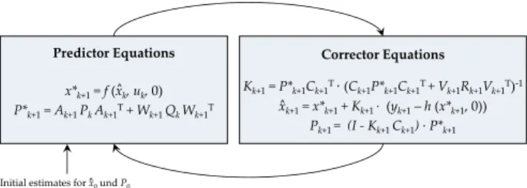
tool in applications for sensor fusion and localization. The equations of the Kalman Filter fall into two groups: “predictor equations” and “corrector equations”. Based on the system input parameters, the current state estimate and error covariance estimate are projected forward to obtain
the predicted a priori estimates for the next time step.
This operation is called “time update”. Following an actual
measurement is incorporated into the a priori estimate to
obtain an improved a posteriori estimate. In other words
the measurements adjust the predicted estimate at that time, so that this operation is denoted “measurement update”.
As initial values for the primary estimation xˆ0 and P0 are
passed. After each time and measurement update pair, the
process is repeated with the previousa posteriori estimates.
This recursive nature is one of the appealing features of the Kalman Filter and the essential advantage over other stochas-tic estimation methods. The filter recursively conditions the current estimate on all of the past measurements and can be used in real-time applications.
The basic filter is well-established, if the state transition and the observation models are linear distributions. In the
case, if the process to be estimated and/or the measurement
relationship to the process is specified by a non-linear
stochastic difference equation, the Extended Kalman Filter
(EKF) can be applied. This filtering is based on linearizing a non-linear system model around the previous estimate using partial derivatives of the process and measurement function. Fig. 1 shows a complete picture of the operations of the EKF by presenting the specific predictor and corrector
equations. The time update projects the a priori state and
covariance estimates forward from time step to step. The first task during the measurement update is to compute the
Kalman gainKk. The next step is to generate ana posteriori
The final step is to obtain the corresponding error covariance
estimate Pk+1 for the next iteration.
Predictor Equations x*k+1= f (xk, uk, 0) P*k+1= Ak+1 PkAk+1T+ Wk+1 QkWk+1T Corrector Equations Kk+1= P*k+1Ck+1T ∙(Ck+1P*k+1Ck+1T + Vk+1Rk+1Vk+1T)‐1 xk+1= x*k+1+ Kk+1 ∙(yk+1– h (x*k+1, 0)) Pk+1 = (I ‐Kk+1 Ck+1) ∙P*k+1 ^ ^
Initial estimates forx^0und P0
Fig. 1. Time update and measurement update equations of the Extended Kalman Filter
A. Design of the Extended Kalman Filter
The Extended Kalman Filter is suitable to determine the x-and y-position of the mobile tag with the measured distances to at least three anchors. Using the trilateration method the
anchor distancesri are calculated as follow:
ri=
√︁
(px−ax,i)2+(py−ay,i)2, (2)
where (ax,i,ay,i) are the x- and y-positions of anchor i and
(px,py) represents the x- and y-position of the mobile tag to
be located.
To gain the unknown tag position, the equations in (2) are
solved for pxand py, and are transformed in matrices:
H · (︃ px py )︃ =zwithH= ⎛ ⎜ ⎜ ⎜ ⎜ ⎜ ⎜ ⎜ ⎜ ⎜ ⎜ ⎝ 2·ax,1−2·ax,2 2·ay,1−2·ay,2 .. . ... 2·ax,1−2·ax,n 2·ay,1−2·ay,n ⎞ ⎟ ⎟ ⎟ ⎟ ⎟ ⎟ ⎟ ⎟ ⎟ ⎟ ⎠ , andz= ⎛ ⎜ ⎜ ⎜ ⎜ ⎜ ⎜ ⎜ ⎜ ⎜ ⎜ ⎝ r22−r12+ax,12−ax,22+ay,12−ay,22 .. . rn2−r12+ax,12−ax,n2+ay,12−ay,n2 ⎞ ⎟ ⎟ ⎟ ⎟ ⎟ ⎟ ⎟ ⎟ ⎟ ⎟ ⎠ , (3)
wheren is the overall number of anchor nodes. Eqn. 3 can
be solved using the method of least squares:
(︃ ˆ px ˆ py )︃ =(HTH)−1HT ·z (4)
For location tracking using EKF, Eqn. (3) needs only to
be solved for the initial estimate xˆ0. In this work the raw
trilateration (3) is also used as reference. The EKF addresses the general problem of estimating the interior process state of a time-discrete controlled process, that is governed by
non-linear difference equations:
˜
xk+1 = f(xˆk,uk,wk),
˜
yk+1 =h(x˜k+1,vk+1).
(5)
The state vector contains the tag position xk = (px,py)T.
The optional input control vectoruk=(vx,vy)T contains the
desired velocity of the tag. These values are set to zero, if
the input is unknown. The observation vector yk represents
the observations at the given system and defines the entry parameters of the filter, in this case the results of the range
measurements. The process function f relates the state at the
previous time stepkto the state at the next step k+1. The
measurement functionhacts as a connector between xkand
yk. The notationx˜kand˜ykdenotes the approximateda priori
state and observation, xˆk typifies the a posteriori estimate
of the previous step. Referring to the state estimation, the process is characterized with the stochastic random variables
wk andvk representing the process and measurement noise.
They are assumed to be independent, white and normal
probably distributed with given covariance matrices Qk and
Rk. To estimate a process with non-linear relationships the
equations in (5) must be linearized as follow:
xk+1 ≈x˜k+1+Ak+1·(xk−xˆk)+Wk+1·wk
yk+1 ≈˜yk+1+Ck+1·(xk+1−x˜k+1)+Vk+1·vk+1, (6)
where Ak+1,Wk+1,Ck+1 andVk+1 are Jacobian matrices with
the partial derivatives:
Ak+1= ∂∂xf(xˆk,uk,0) Wk+1= ∂∂wf(xˆk,uk,0)
Ck+1=∂∂hx(x˜k+1,0) Vk+1= ∂∂hv(x˜k+1,0).
(7) Because in the analyzed system the predictor equation
con-tains a linear relationship, the process function f can be
expressed as a linear equation:
xk+1=Axk+Buk+wk, (8)
where the transition matrix A andBare defined as:
A= (︃ 1 0 0 1 )︃ , B= (︃ T 0 0 T )︃ , (9)
whereT is the constant sampling time.
The observation vector yk contains the current measured
distances:
yk=(︀r1 · · · rn)︀ T
. (10)
The initial state estimate xˆ0 is calculated based on (3). For
the subsequent estimation of the tag position (px,py) the
functional values of the non-linear measurement function
h must be approached to the real position. The function
h comprises the trilateration equations (2) and calculates
the approximated measurement y˜k+1 to correct the present
estimation x˜k+1. The equation ˜yk+1 = h(x˜k+1,vk+1) is given
as: ⎛ ⎜ ⎜ ⎜ ⎜ ⎜ ⎜ ⎜ ⎜ ⎜ ⎜ ⎝ ˆ r1 .. . ˆ rn ⎞ ⎟ ⎟ ⎟ ⎟ ⎟ ⎟ ⎟ ⎟ ⎟ ⎟ ⎠ = ⎛ ⎜ ⎜ ⎜ ⎜ ⎜ ⎜ ⎜ ⎜ ⎜ ⎜ ⎜ ⎝ √︀ ( ˜px−ax,1)2+( ˜py−ay,1)2 .. . √︀ ( ˜px−ax,n)2+( ˜py−ay,n)2 ⎞ ⎟ ⎟ ⎟ ⎟ ⎟ ⎟ ⎟ ⎟ ⎟ ⎟ ⎟ ⎠ +vk+1. (11)
The related Jacobian matrix Ck+1 = ∂∂hx(x˜k,0) describes the
partial derivatives of h with respect to x:
Ck+1= ⎛ ⎜ ⎜ ⎜ ⎜ ⎜ ⎜ ⎜ ⎜ ⎜ ⎜ ⎜ ⎜ ⎝ ∂ˆr1 ∂p˜x ∂ˆr1 ∂p˜y .. . ... ∂ˆrn ∂p˜x ∂ˆrn ∂p˜y ⎞ ⎟ ⎟ ⎟ ⎟ ⎟ ⎟ ⎟ ⎟ ⎟ ⎟ ⎟ ⎟ ⎠ with ∂ˆri ∂p˜x = ˜ px−ax,i √ ( ˜px−ax,i)2+( ˜py−ay,i)2 ∂rˆi ∂p˜y = ˜ py−ay,i √ ( ˜px−ax,i)2+( ˜py−ay,i)2 . (12)
Given that h contains non-linear difference equations the
parametersri as well as the Jacobian matrix Ck+1 must be
B. Detection of NLOS range measurements
The range measurements can be modeled as
ri,k=di,k+ni,k+ei,k,NLOS, (13)
where ri,k is the range measurement to node i at sample
time k, di,k is the real distance, ni,k is the measurement
noise and ei,k,NLOS is the measurement error due to NLOS.
The measurement noise is modeled as Gaussian noiseni,k∼
𝒩(0, σi), where σi can be identified by experiments.
Two different techniques for NLOS detection are studied.
Both methods use the time update of the Kalman Filter to estimate the position of the vehicle
˜
xk+1=Axk+Buk, (14)
and to calculate the range estimates as ˆ
ri,k+1=
√︁
( ˜px,k+1−ax,i)2+( ˜py,k+1−ay,i)2. (15)
The first method compares the range estimates to the real range measurements in order to detect NLOS:
ˆ
ei,k+1=ri,k+1−riˆ,k+1 (16)
Assuming small tracking errors ˆri,k+1≈di,k+1 and comparing
(13) with (16) leads to ˆ
ei,k+1≈ni,k+ei,k,NLOS (17)
NLOS is detected, if the error is positive and larger than a range error limit:
ˆ
ei,k+1≥ei,limit : NLOS
ˆ
ei,k+1<ei,limit : LOS,
(18)
where the error limitei,limit is obtained experimentally.
The second technique use the standard deviation of the estimated range measurement errors (16) to detect NLOS as described in [13]. Under NLOS condition, the signal propagation path changes quickly, when a vehicle moves. Owing to this fact, the standard deviation of the range measurement errors is significantly larger in case of NLOS than in case of LOS condition. The standard deviation of the range errors (16) is estimated periodically in a floating window: ˆ σi= ⎯ ⎸ ⎷ 1 K k ∑︁ j=k−K+1 ˆ e2i,j (19)
where K is the size of the floating window. Comparing ˆσi
withσi detects NLOS conditions:
ˆ
σi≥γσi : NLOS
ˆ
σi< γσi : LOS (20)
The parameter γ can be find out experimentally. γ > 1
has to be chosen to reduce the probability of false alarm.
The effectiveness of both techniques depends on the tracking
performance of the EKF and on the quality of the initial state estimate xˆ0.
C. Mitigation of NLOS range measurements
Two slightly different methods for mitigation of NLOS
range measurements have been studied. Both techniques use the Biased Kalman Filter. If NLOS is detected, the
corre-sponding elements of the measurement covariance matrix R
are increased: R= ⎛ ⎜ ⎜ ⎜ ⎜ ⎜ ⎜ ⎜ ⎜ ⎜ ⎜ ⎜ ⎜ ⎜ ⎜ ⎜ ⎜ ⎝ σ2 r,1 0 · · · 0 0 σ2 r,2 · · · 0 .. . ... ... ... 0 0 · · · σ2r,n ⎞ ⎟ ⎟ ⎟ ⎟ ⎟ ⎟ ⎟ ⎟ ⎟ ⎟ ⎟ ⎟ ⎟ ⎟ ⎟ ⎟ ⎠ (21)
The first technique (BEKF1) uses the estimated range error
obtained from (16) to increase the covariance of R:
σ2 r,i= ⎧ ⎪ ⎪ ⎨ ⎪ ⎪ ⎩ βeiσˆ 2 i : NLOS σ2 i : LOS , (22)
whereβis chosen by experiments to give a good tracking
per-formance. The second method (BEKF2) uses the estimated
covariance to increase the elements ofR:
σ2 r,i= ⎧ ⎪ ⎪ ⎨ ⎪ ⎪ ⎩ ασˆ2 i : NLOS σ2 i : LOS , (23) where ˆσ2
i is obtained from (19) and αis chosen by
experi-ments to give a good tracking performance.
These techniques are compared with an EKF, which dis-cards NLOS range measurements. The NLOS measurements are discarded by adapting the output equation of the EKF.
Only LOS measurements are included in yk andCk of (10)
and (12).
V. ExperimentResults andPerformanceAnalysis A. Experimental Setup
In a test series, the position of a forklift truck is tracked using the described method. The experiments are carried out at a demonstration storage of the Fraunhofer-Institute for Ma-terial Flow and Logistics in Dortmund Germany. The forklift truck moves in automatic mode along a half oval course. It is controlled by laser triangulation, which has a tracking performance better than a few cm. The video attachment of the paper shows the forklift truck moving along this course. The standard nanoLOC development kit which contains five sensor boards with sleeve dipole omnidirectional antennas is utilized for the experiment. Four anchor nodes are placed at
the edges of the course. The sampling timeT is chosen to
0.3 s. Several experiments with different NLOS conditions
have been performed to evaluate the effectiveness of the
proposed techniques. The measured range data are logged into a file for later analysis. The proposed NLOS mitigation techniques are implemented in Matlab and are evaluated offline.
B. Parameter Tuning
The effect of the Kalman estimation depends significantly
on the parameters of the covariance matrices. To preferably gain an exact estimation, appropriate values for the process
Rkmust be detected. The process noise covariance represents
the accuracy of the estimates for the interior process state. The measurement noise covariance depends directly on the environment of the range measurements. Several experiments
with different anchors in a static environment show
covari-ances in a range between 0.0216 m2and 0.354 m2. The
mea-surement noise covariance is chosen withσ2
i =0.1328 m
2 as
mean variance of all experiments. These two matrices have a large impact in progress of the error covariance estimate
Pk, whose initial value is assumed to P0=I·10−2.
The parameters have been chosen by experiments to
ei,limit = 5 m, α = 1, K = 10, β = 1 m−1 and γ = 3 .
These parameters show the best tracking performance for the associated methods.
C. Experimental Results
Several experiments with different NLOS conditions have
been performed to evaluate the effectiveness of the proposed
techniques. In all experiments anchor node 1 is blocked manually with a sheet of metal several times during the motion of the forklift truck. The results of three experiments are summarized in Table I. Fig. 2 to Fig. 5 show the results of the first experiment. The LOS was blocked manually several times in intervals of 5 s. The red line shows the course of the forklift truck, which is controlled by laser triangulation. The raw trilateration is shown with green dots and calculated with Eqn. (4). Owing to the measurement noise of the range measurements, the raw trilateration is spread over the whole area. In all figures the raw trilateration is calculated without NLOS mitigation. Owing to this fact, the measured distances to anchor 1 are too large, and the estimated positions are
displaced towards larger values of x and y. Several of the
trilateration points are out of the range of the axis.
Fig. 2 shows the results of the EKF without NLOS mitigation. The estimated position of the EKF is shown as blue line. Fig. 2 shows that NLOS leads to worse tracking performance, if an unmodified EKF is applied. NLOS dis-places the estimated position in the opposite direction of the related anchor node.
14 16 18 20 22 24 26 28 30 32 34 6 7 8 9 10 11 12 13 14 15 position x (m) position y (m) EKF estimation raw trilateration real path anchor nodes 3 4 1 2
Fig. 2. Tracking results of EKF without NLOS mitigation
The same data are used for the EKF and NLOS measure-ment exclusion shown in Fig. 3. The tracking performance is much better than using an unmodified EKF. In environments with a large number of NLOS conditions, the lack of LOS measurements can lead to estimation failure. In this setup
14 16 18 20 22 24 26 28 30 32 34 6 7 8 9 10 11 12 13 14 15 position x (m) position y (m) real path raw trilateration EKF estimation anchor nodes 2 4 3 1
Fig. 3. Tracking results of EKF with NLOS measurement rejection
measurements with ˆei >10 m are discarded. Lowering this
limit lead to a complete failure of the location estimation. In cases where the tracking error becomes high, the range error estimates increases and all measurements are discarded.
The BEKF uses both LOS and NLOS range measure-ments. NLOS measurements are less weighted than LOS measurements. Fig. 4. shows the results from using BEKF with NLOS mitigation method BEKF1. The tracking
perfor-14 16 18 20 22 24 26 28 30 32 34 6 7 8 9 10 11 12 13 14 15 position x (m) position y (m) real path raw trilateration EKF estimation anchor nodes 2 1 4 3
Fig. 4. Tracking results of BEKF1
mance is better than using an unmodified EKF. The filter reacts immediately after detecting a NLOS condition.
Fig. 5 shows the results from using NLOS mitigation method BEKF2. The tracking performance is slightly better than method BEKF1. Fig. 6 shows the distribution of the
14 16 18 20 22 24 26 28 30 32 34 6 7 8 9 10 11 12 13 14 15 position x (m) position y (m) real path trilateration EKF estimation anchor nodes 2 1 4 3
Fig. 5. Tracking results of BEKF2
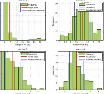
true range errorseiof the four anchor nodes. The distribution
shows NLOS condition in anchor node 1 and biased range errors in the other anchor nodes, which may be caused by multipath signal propagation.
0 5 10 15 20 25 30 0 10 20 30 40 50 60 range error (m) frequency anchor 1 −1 −0.5 0 0.5 1 1.5 2 2.5 0 5 10 15 20 range error (m) frequency anchor 2 0 1 2 3 4 0 5 10 15 20 range error (m) frequency anchor 3 −1 0 1 2 3 0 5 10 15 20 25 range error (m) frequency anchor 4 frequency mean error standard deviation frequency mean error standard deviation frequency mean error standard deviation frequency mean error standard deviation
Fig. 6. Histogram of true range errorsei
TABLE I
Mean absolute error and standard deviation
# EKF EKF disc. BEKF1 BEKF2 mean abs error 1 1,76 0,59 0,47 0,28 standard deviation 1,36 1,07 1,21 0,91 mean abs error 2 0,51 0,51 0,46 0,38 standard deviation 0,81 0,81 0,78 0,75 mean abs error 3 0,56 0,58 0,51 0,58 standard deviation 1,52 1,55 1,43 1,55
The mean absolute error and the standard deviation of the errors are listed in Table I, for three experiments. In the first experiment LOS was blocked several times in intervals of 5 s. In experiment 2 LOS is blocked for 4 s just before and after the curve. In the third experiment LOS is blocked for 8 s in the second half of the course. BEKF2 shows the best tracking performance in most cases.
VI. Conclusions
In this paper, location tracking of an forklift truck using range measurements and Biased Extended Kalman Filtering with NLOS mitigation is described. The main source for ranging errors in indoor environments is NLOS and
multi-path signal propagation. Two different techniques for NLOS
mitigation have been evaluated and compared with an un-modified EKF and with an EKF with NLOS measurement exclusion. Discarding NLOS measurements is the easiest way to handle NLOS range measurements. In environments with a large number of NLOS conditions, the lack of LOS measurements may lead to estimation failure. In cases where the tracking error becomes high, the range error estimates increases and all measurements are discarded.
The BEKF uses LOS as well as NLOS range measure-ments. NLOS measurements are less weighted than LOS measurements. The first technique (BEKF1) uses the
esti-mated range error directly. The second technique (BEKF2) calculates the standard deviation of the range errors. Both
techniques are more robust than EKF and offer better
track-ing performance. The first technique reacts faster on NLOS. The second technique leads to a slightly better tracking performance.
References
[1] Z. Sahinoglu and S. Gezici, “Ranging in the IEEE 802.15.4a Stan-dard,” in Proceedings of the IEEE Annual Wireless and Microwave
Technology Conference, WAMICON ’06, Clearwater, Florida, USA,
Dec. 2006, pp. 1–5.
[2] J. Graefenstein, A. Albert, and P. Biber, “Radiation Pattern Correlation for Mobile Robot Localization in Low Power Wireless Networks,” in
Proceedings of the 2009 IEEE International Conference on Robotics
and Automation, May 2009, pp. 3545–3550.
[3] S. Spieker and C. Röhrig, “Localization of Pallets in Warehouses using Wireless Sensor Networks,” inProceedings of the 16th Mediterranean
Conference on Control and Automation, Corsica, France, Jun. 2008,
pp. 1833–1838.
[4] C. Röhrig and S. Spieker, “Tracking of Transport Vehicles for Warehouse Management using a Wireless Sensor Network,” in2008
IEEE/RSJ International Conference on Intelligent Robots and Systems
(IROS 2008), Nice, France, Sep. 2008, pp. 3260–3265.
[5] M. Vossiek, L. Wiebking, P. Gulden, J. Wieghardt, C. Hoffmann, and P. Heide, “Wireless Local Positioning,”Microwave Magazine, vol. 4, no. 4, pp. 77– 86, Dec. 2003.
[6] L. Hu and D. Evans, “Localization for Mobile Sensor Networks,” in
Proceedings of the 10th Annual International Conference on Mobile
Computing and Networking, 2004, pp. 45–57.
[7] N. Patwari, A. O. Hero, M. Perkins, N. S. Correal, and R. O’Dea, “Relative Location Estimation in Wireless Sensor Networks,”IEEE
Transactions on Signal Processing, vol. 51, no. 8, pp. 2137–2148,
2003.
[8] C. Röhrig and F. Künemund, “Estimation of Position and Orientation of Mobile Systems in a Wireless LAN,” inProceedings of the 46th
IEEE Conference on Decision and Control, New Orleans, USA, Dec.
2007, pp. 4932–4937.
[9] N. B. Priyantha, A. K. L. Miu, H. Balakrishnan, and S. Teller, “The Cricket Compass for Context-aware Mobile Applications,” in
Proceedings of the 7th Annual International Conference on Mobile
Computing and Networking, Rome, Italy, Jul. 2001, pp. 1–14.
[10] P. Alriksson and A. Rantzer, “Experimental Evaluation of a Distributed Kalman Filter Algorithm,” inProceedings of the 46th IEEE
Confer-ence on Decision and Control, New Orleans, Dec. 2007, pp. 5499–
5504.
[11] S. Gezici, Zhi Tian, G. Giannakis, H. Kobayashi, A. Molisch, H. Poor, and Z. Sahinoglu, “Localization via Ultra-wideband Radios: A Look at Positioning Aspects for Future Sensor Networks,”Signal Processing
Magazine, vol. 22, no. 4, pp. 70–84, Jul. 2005.
[12] J. Fernández-Madrigal, E. Cruz, J. González, C. Galindo, and J. Blanco, “Application of UWB and GPS Technologies for Vehicle Localization in Combined Indoor-Outdoor Environments,” in Proceed-ings of the International Symposium on Signal Processing and its
Applications, Sharja, United Arab Emirates, Feb. 2007.
[13] B. L. Le, K. Ahmed, and H. Tsuji, “Mobile Location Estimator with NLOS Mitigation Using Kalman Filtering,” in Proceedings of the
Wireless Communications and Networking Conference, vol. 3, Mar.
2003, pp. 1969–1973.
[14] “Real Time Location Systems (RTLS),” Nanotron Technologies GmbH, Berlin, Germany, White paper NA-06-0248-0391-1.02, Apr. 2007.
[15] “nanoloc TRX Transceiver (NA5TR1),” Nanotron Technologies GmbH, Berlin, Germany, Datasheet NA-06-0230-0388-2.00, Apr. 2008.
[16] “nanoloc Development Kit User Guide,” Nanotron Technologies GmbH, Berlin, Germany, Technical Report NA-06-0230-0402-1.03, Feb. 2007.