IMT School for Advanced Studies
Lucca
Arenberg Doctoral School
Faculty of Engineering Science
Proximal envelopes: Smooth optimization
algorithms for nonsmooth problems
Lorenzo Stella
Supervisors:
Prof. Panagiotis Patrinos (KU Leuven) Prof. Alberto Bemporad (IMT Lucca)
Dissertation presented in partial fulfillment of the requirements for: PhD in Computer, Decision and Systems Science, XXVIII Cycle Degree of Doctor of Engineering Science (PhD): Electrical Engineering
The dissertation of Lorenzo Stella is approved.
Program Coordinator: Prof. Pietro Pietrini, IMT Lucca
Supervisor: Prof. Panagiotis Patrinos, KU Leuven
Supervisor: Prof. Alberto Bemporad, IMT Lucca
The dissertation of Lorenzo Stella has been reviewed by:
Prof. Pontus Giselsson, Lund University
Prof. Johan Suykens, KU Leuven
IMT School for Advanced Studies, Lucca
2017
Contents
List of Figures xi
List of Tables xii
Acknowledgements xiii
Vita and Publications xiv
Abstract xvi Notation xvii 1 Introduction 1 1.1 Structured optimization . . . 2 1.2 Proximal algorithms . . . 5 1.3 Proximal envelopes . . . 8
1.4 Contributions and organization . . . 11
1.A Tools and notation . . . 13
1.A.1 Convex and variational analysis tools . . . 13
1.A.2 Continuity and (generalized) differentiability . . . . 16
1.A.3 Convergence rates . . . 18
2 Forward-backward quasi-Newton methods 20 2.1 Introduction . . . 20
2.1.1 Forward-backward splitting . . . 23
2.2 Forward-backward envelope . . . 26
2.2.1 Basic inequalities . . . 26
2.2.2 First- and second-order properties . . . 31
2.2.3 Interpretations . . . 36
2.3 Forward-backward line-search methods . . . 37
2.3.1 Convergence in the convex case . . . 44
2.3.2 Convergence under KL assumption . . . 47
2.4 Quasi-Newton methods . . . 52
2.4.1 BFGS . . . 57
2.4.2 L-BFGS . . . 59
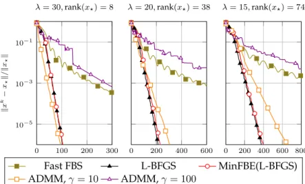
2.5 Simulations . . . 60
2.5.1 Lasso . . . 60
2.5.2 Sparse logistic regression . . . 62
2.5.3 Group lasso . . . 64
2.5.4 Matrix completion . . . 66
2.5.5 Image restoration . . . 68
2.6 Conclusions . . . 69
2.A Additional results . . . 71
3 A simple and efficient algorithm for nonlinear MPC 76 3.1 Introduction . . . 76
3.1.1 Problems framework and motivation . . . 77
3.1.2 Contributions . . . 78
3.2 Newton-type forward-backward method . . . 79
3.2.1 Newton-type methods on generalized equations . . 80
3.2.2 Forward-backward envelope . . . 81
3.2.3 A superlinearly convergent algorithm based on FBS 83 3.3 Nonlinear MPC . . . 88
3.3.1 Handling state constraints . . . 89
3.4 Numerical Simulations . . . 92
3.4.2 Results . . . 95
3.5 Conclusions . . . 96
4 Newton-type alternating minimization algorithm 99 4.1 Introduction . . . 99
4.1.1 Contributions . . . 101
4.2 Background and proposed algorithm . . . 102
4.2.1 Newton-type alternating minimization algorithm . 105 4.2.2 Quasi-Newton directions . . . 107
4.3 Alternating minimization envelope . . . 109
4.3.1 Analogy with the dual Moreau envelope . . . 111
4.4 Convergence . . . 112
4.5 First- and second-order properties . . . 118
4.6 Superlinear convergence . . . 124
4.7 Simulations . . . 127
4.7.1 Linear MPC . . . 128
4.8 Conclusions . . . 133
4.A Additional results . . . 135
5 Fast Douglas-Rachford splitting algorithm 139 5.1 Introduction . . . 139
5.1.1 Contributions . . . 141
5.2 Douglas-Rachford envelope . . . 142
5.2.1 DRS as a variable-metric gradient method . . . 145
5.2.2 Connection between DRS and FBS . . . 146
5.3 Convergence rate and stepsize selection in DRS . . . 148
5.4 Fast Douglas-Rachford splitting . . . 152
5.5 Simulations . . . 154
5.5.1 Box-constrained QP . . . 154
5.5.2 Lasso . . . 155
5.6 Conclusions and future work . . . 156
6 Conclusions and outlook 161
6.1 Future directions . . . 164
List of Figures
1 Forward-backward splitting as majorization-minimization 25
2 Forward-backward envelope construction . . . 27
3 Forward-backward envelope bounds . . . 28
4 Lasso: performance on one instance . . . 62
5 Lasso: performance on multiple instances . . . 63
6 Group lasso: performance of the algorithms . . . 66
7 Matrix completion: performance of the algorithms . . . 68
8 Image restoration: performance of the algorithms . . . 69
9 Image restoration: original and recovered images . . . 70
10 Spring-mass system: initial position . . . 95
11 Spring-mass system: convergence of the algorithms . . . . 97
12 Spring-mass system: CPU time for closed-loop simulations 97 13 Spring-mass system: effect of soft-state constraints . . . 98
14 Oscillating masses: schematic representation . . . 133
15 Oscillating masses: average and maximum CPU time . . . 134
16 Douglas-Rachford envelope for box QP . . . 146
17 Box QP: performance of (fast) DRS . . . 155
18 Lasso: stepsize selection in DRS . . . 157
List of Tables
2 Sparse logistic regression: performance of the algorithms . 65 3 Aircraft control: performance of the algorithms . . . 132 4 Comparison between the proposed algorithms . . . 163
Acknowledgements
I would first like to express my sincere gratitude to Prof. Pana-giotis Patrinos: none of this would be possible without his directions, support, and constant motivation and ideas. Most importantly, Panos introduced me to a very exciting area of research, and provided me with tools that I alone would oth-erwise hardly be able to master. It was an honor and a privi-lege to closely work with him.
I am also greatful to Prof. Alberto Bemporad for letting me be part of the DYSCO research unit at IMT Lucca: his vast experience and constructive advices have been fundamental throughout these years.
I greatfully acknowledge the ESAT/Stadius division of KU Leuven, directed by Prof. Marc Moonen, and all its members and staff with which I had the pleasure to meet, discuss, col-laborate. They welcomed me and supported me throughout the final year of PhD, and I am fully indebted with them. Special thanks go to Andreas for lending me his math skills in numerous occasions, and his TEX typesettings. Thanks to all my close friends and colleagues from IMT Lucca and KU Leuven, with whom I shared more than I could list in a page. Thank you for coffee, drinks, laughters, ping pong, board games, calcetto, LAN parties, NERF guns, crazy talks and late night office madness: (in alphabetical order) Ajay, Al-berto, Alessio, Andrea, Andreas, Benedetta, Bertrand, Chris, Daniele, Davide, Duccio, Fabiana, Francesco, Giada, Gionata, Giovanni, Luca, Marco, Michela, Pantelis, Pietro, Puya, Rita, Samuele. It really was a wonderful time.
Vita
Dec. 12, 1985 Born in Florence, Italy 2004 – 2008 B.Sc. in Computer ScienceFinal mark: 110/110 University of Florence, Italy 2008 – 2011 M.Sc. in Computer Science
Final mark: 110/110 cum laude University of Florence, Italy
2013 – 2017 Ph.D. in Computer, Decision and Systems Science IMT Lucca, Italy
09/15 – 01/16 Visiting student, KU Leuven, Belgium ESAT – Department of Electrical Engineering Since 03/16 Ph.D. student jointly at KU Leuven, Belgium ESAT – Department of Electrical Engineering
Publications
Journal papers
1. L. Stella, A. Themelis and P. Patrinos. Forward-backward quasi-Newton methods for nonsmooth optimization problems. Computational Optimiza-tion and ApplicaOptimiza-tions, 67(3):443–487, 2017.10.1007/s10589-017-9912-y.
2. L. Stella, A. Themelis and P. Patrinos. Newton-type alternating minimiza-tion algorithm for convex optimizaminimiza-tion.Submitted, 2017.
3. A. Themelis, L. Stella and P. Patrinos. Forward-backward envelope for the sum of two nonconvex functions: Further properties and nonmonotone line-search algorithms.arXiv:1606.06256, 2016.
Conference proceedings
1. L. Stella, A. Themelis, P. Sopasakis and P. Patrinos. A simple and efficient algorithm for nonlinear model predictive control.Submitted, 2017.
2. P. Latafat, L. Stella and P. Patrinos. New primal-dual proximal algorithms for distributed optimization.55th IEEE Conference on Decision and Control,
1959–1964, 2016.10.1109/CDC.2016.7798551.
3. P. Patrinos, L. Stella and A. Bemporad. Douglas-Rachford splitting: com-plexity estimates and accelerated variants.53rd IEEE Conference on Decision and Control, 4234–4239, 2014.10.1109/CDC.2014.7040049.
Working papers
1. P. Patrinos, L. Stella and A. Bemporad. Forward-backward truncated New-ton methods for convex composite optimization.arXiv:1402.6655, 2014.
Abstract
Nonsmooth optimization problems arise in an ever-growing number of applications in science and engineering. Proxi-mal (or splitting) algorithms are a general approach to a va-riety of nonsmooth problems, but as with all first order me-thods their convergence properties are severely affected by ill conditioning of the problem. In this thesis, an interpreta-tion to proximal algorithms as unconstrained gradient meth-ods over an associated function function is provided. Such functions are called proximal envelopes, in analogy with the
well-known Moreau envelope. Proximal envelopes provide a link between nonsmooth and smooth optimization, and al-low for the application of more efficient and robust smooth optimization algorithms to the solution of nonsmooth, pos-sibly constrained problems. We consider the case of the for-ward-backward and Douglas-Rachford splitting methods. In the first case, based on generalized differentiability properties on the original problem terms, we devise superlinearly con-vergent line-search algorithms based on quasi-Newton direc-tions, that use the same oracle as the forward-backward split-ting; furthermore, the analysis is extended to the case where the dual problem is concerned. In the second case a global convergence rate for the Douglas-Rachford splitting is ob-tained, while an optimal stepsize selection strategy and an accelerated variant of the method is proposed.
Notation
R The real line.R Extended real lineR∪ {+∞}. R+ Non-negative real line.
Γ0(E) Proper, closed, convex functions overE.
C1(E) Continuously differentiable functions overE.
C2(E) Twice continuously differentiable functions overE.
CL1,1(E) Functions overEwithL-Lipschitz gradient.
A⇒B Set-valued mapping between setsAandB. δS Indicator function of setS.
ΠS Projection mapping onto setS.
∂f Subdifferential mapping off.
proxγf Proximal mapping off with stepsizeγ. fixT Set of fixed-points ofT.
zerT Set of zeros ofT. A> Transpose of matrixA.
A† Moore-Penrose pseudo-inverse ofA.
range(A) Range (image) ofA.
null(A) Null space ofA.
λmin(A) Minimum eigenvalue ofA.
λmax(A) Maximum eigenvalue ofA.
σi(A) i-th largest singular value ofA.
JF(x) Jacobian ofF atx.
d2f(x
|v) Second epi-derivative off atxforv. f∗ Convex conjugate function of functionf.
Lγ Augmented Lagrangian function with parameterγ.
fγ Moreau envelope offwith parameterγ.
ϕFB
γ Forward-backward envelope ofϕwith parameterγ.
ϕDRγ Douglas-Rachford envelope ofϕwith parameterγ.
ADMM Alternating direction method of multipliers. ALM Augmented Lagrangian method.
AMA Alternating minimization algorithm. DRE Douglas-Rachford envelope.
DRS Douglas-Rachford splitting. FBE Forward-backward envelope. FBS Forward-backward splitting. MPC Model predictive control.
NMPC Nonlinear model predictive control. PMA Proximal minimization algorithm.
Chapter 1
Introduction
Optimization problems are ubiquitous in science and engineering. Clas-sically, optimization was regarded as the minimization of smooth func-tions: while the gradient method serves as a simple basic approach to this class of problems, much more efficient algorithms are obtained by con-sidering directions other than the steepest descent one, for example by exploiting second-order information on the cost function like in Newton-type methods. However, nowadays an ever-growing number of applica-tions fundamentally relies on nosmoothness to enforce prior knowledge in the problem solution. For this reason new, simple iteration schemes have been designed that usually go by the name ofproximal algorithmsor splitting methods. These are essentially fixed-point iterations for solving a
nonsmooth, nonlinear system of equations defining the stationary points of the cost function. As such, their iterations are very simple and ideal for embedded applications and large-scale problems.
In this thesis we introduce the concept ofproximal envelopes: these
extend and generalize the concept ofMoreau envelope, a very well known
object in convex optimization, and allow to easily reformulate nonsmooth (possibly constrained) problems as smooth unconstrained ones. As a consequence, new efficient algorithms for certain types of nonsmooth,
nonconvex optimization problem are developed and analyzed. The pro-posed methods combine the modern approach of proximal algorithms, which are first order methods, with classical techniques for smooth un-constrained optimization that allow for fast asymptotic convergence. The rest of this chapter serves both as introduction for terminology and back-ground notions, as well as to motivate and introduce the idea of proximal envelopes, and to summarize the contributions of the thesis.Section 1.A contains a summary of the mathematical tools which are used through-out the thesis, and the relative notation.
1.1
Structured optimization
In this thesis we are essentially concerned with problems of the form
minimize
x ϕ(x) =f(x) +g(x), (1.1)
wheref is a smooth (possibly nonconvex) function, whilegis a convex (possibly nonsmooth) function.
Regularization methods in machine learning, statistics, signal pro-cessing, often result in problems of the form (1.1). Herefcan be a smooth penalty, or fitting term, composed with a matrix containing the prob-lem data, whilegis a (possibly nonsmooth) regularization term used to enforce some prior knowledge on the problem solution. For example, the`1normg(x) =kxk1 =Pi|xi|is typically used to enforce sparsity:
thelassomodel for sparse linear regression and the sparse logistic model
for classification fit this framework, see [151], [65, §3.4.2, §4.4.4]. The
elastic-netg(x) =λ1kxk1+λ22kxk22combines the`1and Thikonov
regu-larization [164]. If the variablexis partitioned asx= (x1, . . . , xN), then
g(x) =λPN
i=1kxik2is used to enforcegroupsparsity in the solution [65,
§3.8.4]. When the decision variable is a matrixX then thenuclear norm
g(X) = kXk∗ = Piσi(X)(whereσi indicates thei-th singular value)
spectral sense [34]. For example, to find a low-rank approximation of a matrixMfrom a (noisy) incomplete setSof measurements of its entries, one can use
f(X) = X
(i,j)∈S
(Xi,j−Mi,j)2, g(X) =λkXk∗, (1.2)
and problems of this type have applications in collaborative filtering, ma-chine learning, control, remote sensing, and computer vision, see [33,32] and references therein. See [3] for algorithms with application to sparse and low-rank regularization, and [141] for an extension of this frame-work totensors. Matrix decomposition problems are formulated as (1.1)
with
f(X, Y) =1
2kX+Y −Bk 2
F, g(X, Y) =λkXk1+µkYk∗, (1.3)
see [35], and the goal is to approximate matrixB as the sum of a sparse componentX and a low-rank component Y. This has applications in video processing for example, where models such as (1.3) are used to perform background subtraction from sequences of frames [159].
A more general form of optimization problems that we consider is
minimize
x,z f(x) +g(z)
subject toAx+Bz=b,
(1.4)
whereA, Bare linear operators andbis a vector, whilef andgare func-tions defined over appropriate spaces. IfB=−Ithen (1.4) reduces to
minimize
x f(x) +g(Ax−b), (1.5)
and problem (1.5) can be used to perform robust regression using a nons-mooth loss functiongsuch as the`1norm, the Euclidean norm, or
§12] takes the form (1.5), whereg(z) =Pmax
{0,1−z}is the hinge loss. In image and signal processing,Acan be a linear operator that computes finite differences, andg a (group) sparsity inducing penalty, in which case (1.5) is used to denoise a given signal without affecting rapid vari-ations, such as sharp edges in the case of images [134]. Furthermore, if g = δRm
+ is the indicator function of the nonnegative orthant (see Sec-tion 1.A), (1.5) models the minimizaSec-tion off over a polyhedral set – a very large class of problems: quadratic programming (QP) falls into this category, and constrained optimal control problems in the framework of
model predictive control(MPC) very often take this form [114,144].
Convex problems of the form (1.4) easily allow for decentralized or distributed optimization, when the problem terms are appropriately sep-arable [24]: this is achieved through duality, exploiting the idea ofdual decomposition. Suppose thatf(x) = f1(x1) +. . .+fk(xk),i.e., thatf is
separable with respect to a partitioningx= (x1, . . . , xk)of the variable
x. Then it is easy to verify that the dual of (1.4) is minimize
y f
∗
1(A>1y) +. . .+fk∗(Ak>y) +g∗(B>y)− hb, yi, (1.6)
where y is the dual variable, while fi∗ and g∗ are the conjugate func-tionsof fi andg respectively (seeSection 1.A). In this case, when
solv-ing (1.6), all quantities associated withf∗
1, . . . , fk∗(such as gradients) can
be evaluated independently in separate computing nodes, for example distributed over a network. In particular, the data matricesA1, . . . , Ak
can be handled separately by each computing node, avoiding superflu-ous (and often impractical due to size, or impossible due to privacy con-straints) data exchange. In [24,§7] a variety of patterns that allow for distributed computations is discussed; see [19] for a detailed account on parallel and distributed computations in iterative algorithms. Note that the dual of (1.4) dual takes precisely the form (1.1), which is therefore very comprehensive.
1.2
Proximal algorithms
The simplest algorithm to find a solution to (1.1), in the convex case, is arguably thesubgradient method[140,§2], [18,§3]. From a starting point
x0, iterate until convergence
xk+1=xk−γkvk, vk∈∂ϕ(xk), γk >0.
This is recognized as a fixed-point iteration of the subdifferential map-ping. Due to its simplicity, the subgradient method can be applied to a very wide range of problems. Furthermore, in combination with dual de-composition, this approach results in very simple distributed optimiza-tion algorithms [102,103]. However the simplicity of the method comes at the cost of a usually very slow convergence, and quite restrictive as-sumptions to converge in the first place: for example, one must con-sider a diminishing stepsize satisfyingP
kγk2<∞,
P
kγk =∞
(square-summable but not (square-summable), in order to guarantee convergence un-der the assumption of bounded subgradients along the iterates [18, Prop. 3.2.6].
Much stronger convergence properties can be obtained by iterating theresolventof∂ϕinstead, the so-called proximal mapping of ϕ. In the optimization jargon, this has the following expression [101]
proxγϕ(x) = argmin
z
n
ϕ(z) +21γkz−xk2o, γ >0.
Therefore, evaluatingproxγϕ(x)consists of minimizing a regularized
ver-sion off aroundx: when ϕis convex, such approximation is strongly convex and as a consequenceproxγϕ is well defined and has a unique
solution. Note thatγhere plays the role of a stepsize: whenproxγϕ is
applied to a pointx, a smallγ will yield points which are closer tox, while a largeγwill produce a point which is closer to the minimum ofϕ. The proximal mapping is easily computable for several functions [112].
IfS is a set andδS is the indicator function ofS, thenproxγδS = ΠS is the projection ontoS, which is explicitly computable for many types of sets including affine subspaces, halfspaces, boxes,`1 and`2norm balls,
and convex cones such as the nonnegative orthant, second-order cone, positive semidefinite cone, exponential cone. For many other functions the proximal mapping has an explicit expression, such as the`1 norm,
(squared)`2norm, nuclear norm, elastic-net. For convex quadratic
func-tions, evaluating the proximal mapping is a strongly convex quadratic problem and can be either solved exactly using direct methods, or ap-proximately using specialized, very efficient iterative procedures. See [112] for an extensive survey on how proximal mappings can be com-puted. Iterating the proximal mapping yields the so-calledproximal min-imization algorithm(PMA) [129],
xk+1= prox
γkϕ(x
k), γ
k >0, (1.7)
which is known to converge to a solution with virtually no restriction on the sequence of stepsizes [18, Prop. 5.1.3].
However, for structured problems like (1.1) applying PMA is usually not a trivial task: even ifproxγfandproxγgare easily computable,
evalu-atingproxγ(f+g)is much harder in general and likely requires an iterative
procedure. For this reason,splittingalgorithms have been proposed that
tackle (1.1) by acting separately onf andg: in the convex case, such al-gorithms are the optimization counterpart of operator splitting methods for solving monotone inclusion problems [92,57]; see [112] for a survey on proximal algorithms and their applications, [9] for an in-depth theo-retical analysis of proximal algorithms and their connection to operator splitting methods.
Forward-backward splitting. When f is smooth (i.e., with Lipschitz
continuous gradient) andghas an efficiently computable proximal map-ping, one can solve problem (1.1) by alternating gradient (orforward)
steps onfand proximal (orbackward) steps ong:
xk+1= prox
γg(xk−γ∇f(xk)), γ >0. (1.8)
This is known asproximal gradient methodand is a particular case of the
more generalforward-backward splitting(FBS) [27,92]. The reason behind
this terminology is apparent from the optimality condition of the prob-lem defining the proximal operator: ifz = proxγg(x), then necessarily
z =x−γv, withv ∈ ∂g(z),i.e.,zis obtained by animplicit(backward)
subgradient step overg, as opposed to the explicit (forward) step overf. In the convex case, FBS is known to converge under minimal assump-tions forγ ∈(0,2/Lf), whereLf is the Lipschitz constant of∇f, cf. [9,
Cor. 27.9]. Moreover, the objective value converges with global sublin-ear rate and fastvariants of the method exists with an improved rate
[104,155,10,106]. Convergence of FBS has also been shown for noncon-vex problems [6]. When applied to the dual of equality constrained con-vex problems (1.4), FBS results in what is also known asalternating mini-mization algorithm(AMA) [154,11]. The authors of [112] give an overview
of FBS, its interpretations, properties and applications.
Douglas-Rachford splitting. Another method for solving (1.1) is the Douglas-Rachford splitting (DRS) [92], which was introduced in the 1950s in the context of the numerical solution of PDEs [53]. This combines proximal steps with respect to bothf and g, which are assumed to be efficiently computable, as follows:
yk = proxγf(xk),
zk = proxγg(2yk−xk),
xk+1=xk+λk(zk−yk),
(1.9)
whereγ >0and the stepsizesλk ∈[0,2]satisfyPk∈Nλk(2−λk) = +∞.
If the minimum in (1.1) is attained and the relative interiors of the effective domains off andghave a point in common, it is well known that(zk
−yk)
k∈Nconverges to0, and(x
k)
k∈Nconverges to xsuch that
proxγf(x)∈argminϕ[57,58,9]. Therefore(yk)k∈Nand(z
k)
k∈Nconverge to a solution of (1.1). This general form of DRS was proposed by [57,58], where it was shown that DRS is a particular case of the proximal point algorithm. Therefore DRS converges under very general assumptions: for example, unlike the forward-backward splitting (1.8), parameter γ can take any positive value. Very recently, sublinear convergence of DRS with respect to the objective value was shown [44]. When applied to the dual of equality constrained convex problems (1.4), DRS can be shown to be equivalent to thealternating direction method of multipliers(ADMM),
a very well-known algorithm amenable to large-scale problems and dis-tributed optimization [24,112].
1.3
Proximal envelopes
Proximal algorithms, such as FBS and DRS, are first order methods and as such are usually effective at computing low- to medium-precision so-lutions only. More importantly, their convergence speed is heavily af-fected by the conditioning properties of the problem at hand [72,73].
To improve over basic proximal algorithms we will exploit an idea that originates from the following interpretation of the proximal mini-mization algorithm. The value function of the problem definingproxγϕ
is a very well known object in convex optimization, calledMoreau enve-lope[101]: ϕγ(x) = min z n ϕ(z) + 1 2γkz−xk 2o.
It is not hard to verify thatϕγ(x)lower-approximatesϕand shares with
it its (local) minimizers. Furthermore,ϕγ is continuously differentiable
with gradient
Therefore PMA (1.7) can be reformulated as xk+1=xk
−γ∇ϕγ(xk),
i.e., it is the gradient method applied to the Moreau envelope. As such, it
inherits all properties and drawbacks of the gradient method. When the problem is ill-conditioned,i.e., its solutions lie in a region with very steep
and very flat directions (in other words, the problem is badly scaled), then the convergence of gradient methods is known to be severely af-fected: in the case ofC2functions, this reflects on ill-conditioning of the Hessian matrix at the problem solution [16,§1.3]. However since PMA is equivalent to the gradient method on the Moreau envelope, which is a smooth function, more advanced iterative schemes can be borrowed from the classical literature of smooth optimization in order to improve its performance. This simple idea provides a link between nonsmooth and smooth optimization and has led to the discovery of a variety of al-gorithms for problem (1.1), such as semismooth Newton methods [67], variable-metric [22] and quasi-Newton methods [100,36,28], and trust-region methods [135]. When PMA is applied to the dual of an equal-ity constrained problem, then theaugmented Lagrangian method(ALM),
also known asmethod of multipliers, is obtained [127,128]. This fact, in
connection with the above considerations, has been exploited to propose Newton-type versions of the method of multipliers [15]. However, eval-uating the proximal mapping ofϕ=f+g(hence the Moreau envelopeϕγ
and its gradient) is usually nontrivial as we already mentioned: as a con-sequence, a gradient-based iterative algorithm operating on the Moreau envelope will necessarily require inner iterations to evaluate gradients.
In this thesis we introduceproximal envelopefunctions: these
general-ize and extend the concept of Moreau envelope to structured problems such as (1.1). In particular, proximal envelopes
(i) allow to reformulate (1.1), which is nonsmooth and possibly con-strained in general, as an equivalent smooth unconcon-strained
prob-lem (i.e., having the same solutions);
(ii) offer an interpretation of proximal (splitting) algorithms as gradi-ent methods over a smooth function, suggesting the tempting idea of applying much more efficient and robust algorithms from the classical literature of smooth unconstrained optimization: New-ton, quasi-NewNew-ton, limited-memory methods [48, 93, 108], non-linear conjugate gradient methods [71,42,43,76,77], the Barzilai-Borwein method [7,64,125,41], are all viable approaches to mini-mize proximal envelope functions, and therefore solve the original nonsmooth problem.
These features render the analogy with the concept of Moreau envelope apparent: in fact, it is easy to show that the Moreau envelope is a partic-ular case of the proximal envelope functions which are discussed here. However, proximal envelopes (and possibly their gradient) can be evalu-ated at any given point simply using the machinery of the corresponding splitting algorithm. This is in stark contrast with the above mentioned methods based on the Moreau envelope, which usually require an inner iterative procedure.
In particular, we introduce the idea of proximal envelopes in the con-text of FBS and DRS described above, exploit it to obtain algorithms with improved convergence properties, and demonstrate the practical efficacy of this apporach by applying the proposed algorithms to a variety of problems.
In the first case theforward-backward envelope(FBE), first proposed in
[113], allows us to develop line-search algorithms with global conver-gence properties and fast (superlinear) asymptotic rate when Newton-type directions are employed [145,147,146]. This is achieved through the analysis of first- and second-order properties of the FBE, and observing that these are ensured by mild, generalized differentiability assumptions on the original problem. Other approaches have been taken towards the inclusion of second-order information in the iterations of FBS, to improve
convergence [138,12,86,137]. However, algorithms resulting from these approaches have the limitation that they require an inner iterative pro-cedure. Differently, the algorithms presented here rely solely on evalua-tions of the FBE (and possibly its gradient), and because of this they are based on the same type of black-box oracle as FBS. In particular, they do not require any inner iterative procedure. The algorithms based on the FBE which are introduced in this thesis were implemented in ForBES, a software package for MATLAB which is available online1: this contains
generic implementations of the proposed algorithms, and allows to ap-ply them to a variety of applications by specifying the problem terms in (1.1) or (1.4).
In the second case theDouglas-Rachford envelope(DRE) allows to
de-rive a sublinear global convergence rate of orderO(1/k)for the objective
value (a result that was unknown in general until very recently [44]), a linear rate in the strongly convex case, and an optimal stepsize selection for DRS under appropriate assumptions. Furthermore, an accelerated version of the method is derived, with global rateO(1/k2), when one of
the two summands ofϕis quadratic [116].
1.4
Contributions and organization
The contributions and structure of the thesis are outlined as follows. Chapter2, based on [145]: We introduce the forward-backward enve-lope (FBE), which will be exploited heavily troughout the thesis, and an-alyzes its properties. In particular, first- and second-order differentiabil-ity of the FBE are investigated. A gradient-based line-search algorithm, based on the FBE, are then introduced. The proposed algorithm has sim-ilar global convergence properties as FBS (in particular, it enjoys a global sublinear rate in the convex case). Furthermore, superlinear asymptotic convergence of the algorithm is studied when quasi-Newton directions
are employed in the line-search.
Chapter3, based on [147]: We consider another algorithmic scheme, based on forward-backward operations and the FBE, which is conceptu-ally simpler than the one in Chapter2. In particular, no gradient eval-uation of the FBE is performed, hence no second order information on the smooth term of the cost is required. Nevertheless, fast directions can be computed that allow to show superlinear convergence of the iterates. The proposed algorithm is applied to nonlinear MPC problems, which are nonconvex.
Chapter4, based on [146]: Here we are concerned with convex sepa-rable problems with linear equality constraints, and the dual problem is tackled. In this case the FBE is shown to be equivalent to the augmented Lagrangian function of the primal problem, evaluated at certain specific primal points. First- and second-order properties of the FBE are extended to this case, and linked directly to generalized differentiability properties of the primal cost. A similar algorithm to the one in Chapter3is consid-ered in this context, which is an extension of the alternating minimization algorithm. The algorithm converges superlinearly when quasi-Newton directions are considered, and we also show sublinear and linear conver-gence rates under mild assumptions.
Chapter5, based on [116]: We explore the idea of proximal envelopes in the context of the Douglas-Rachford splitting. The analysis is restricted to convex problems, in the case where one term in the objective is smooth: when this is quadratic in particular, then the Douglas-Rachford splitting is equivalent to a gradient method over a smooth convex function. Con-sequently, a sublinear convergence rate is shown for the algorithm, and linear convergence is proved in the strongly convex case. Finally, an op-timal stepsize selection and an accelerated version of the method are pro-posed.
Chapter6contains some final remarks and conclusions, and outlines future research directions.
1.A
Tools and notation
Throughout the thesis,h ·, · iis an inner product over a Euclidean space Eandk · k=ph ·, · iis the associated norm: the exact nature ofEwill be clear from the context. We denote byR=R∪ {−∞,+∞}the extended real line. Functions with values inRare said to beextended real-valued. The set of continuously differentiable functions onEhavingL-Lipschitz continuous gradient (also referred to asL-smooth) is denoted byCL1,1(E).
1.A.1
Convex and variational analysis tools
The following are basic notions in convex analysis, and can be found for example in [17] or [132]. A setCis said to beconvexif any line between
two points in the set lies entirely in the set. Formally, αx+ (1−α)y ∈C, for allx, y∈C.
Theaffine hullof a convex setS ⊆ E, denoted affS, is the intersection of all affine subspaces containingS; equivalently, it is the set of affine combinations (i.e., linear combinations with coefficients summing to1)
of points inS. For a convex setC ⊆ E, therelative interiorofC is the set of pointsx ∈C for which a sphereScentered inxexists, such that S∩affC ⊂ C. Note that while a convex set may have empty interior (think of a proper subspace ofE), the relative interior of a nonempty convex set is always nonempty [17, Prop. 1.3.2].
A functionf :E→Ris said to be convex if
f(αx+ (1−α)y)≤αf(x) + (1−α)f(y), for allx, y∈E, α∈(0,1).
An alternative definition can be given in terms of theepigraph
Thenf is convex if and only ifepif is a convex set. Another important set associated with extended-real-valued functions is theeffective domain, i.e., the subsetdomf = {x∈E|f(x)<+∞} ⊆ E. Iff is convex then domf is necessarily a convex set. Furthermore, we say thatf isproperif domf is nonempty andf is finite ondomf;closedifepif is a closed set inE×R. The family of proper, closed, convex functions defined onE with values inRis indicated asΓ0(E). Functionf is said to bestrongly
convexwith modulusc >0iff−c
2k · k
2is convex.
Given a function honE, the(limiting) subdifferential ∂h of his the set-valued mapping [133, Def. 8.3]
∂h(x) = nv∈E| ∃(xk)k∈N,(v k ∈∂hˆ (xk))k∈Ns.t.x k →x, vk→vo where ˆ ∂h(x) = {v∈E|h(z)≥h(x) +hv, z−xi+o(kz−xk), for allz∈E} is theregular subdifferentialofhatx. This includes the ordinary gradient in the case of continuously differentiable functions, while forg ∈Γ0(E)
it is equivalent to the usual subdifferential for convex functions,i.e.,
∂g(x) = {v∈E|g(y)≥g(x) +hv, y−xi,∀y∈E}.
We denote byzer∂h = {x∈E|0∈∂h(x)} the set ofcritical points of
functionh. A necessary condition for a pointxto be a local minimizer of his thatx∈zer∂ϕ[133, Thm. 10.1]. Ifhis convex then the condition is also sufficient, andxis a global minimizer.
Theproximal mapping[101] ofh, with stepsizeγ >0, is defined as
proxγh(x) = argmin u∈E n h(u) + 1 2γku−xk 2o. (1.10)
theindicator functionof a nonempty setS⊆E,i.e.,
δS(x) =
(
0 ifx∈S,
∞ otherwise,
thenproxγδS = ΠSis the projection ontoSfor anyγ >0. The value func-tion of the optimizafunc-tion problem (1.10) defining the proximal mapping is called theMoreau envelope[101] and is denoted byhγ,i.e.,
hγ(x) = min
u∈E
n
h(u) +21γku−xk2o. (1.11) Properties of the Moreau envelope and the proximal mapping are well documented in the literature [9,133,38,37]. For a closed, proper function h, it holds hγ ≤ h, and hγ(x) = h(x)for any critical point x. If his
also convex, thenproxγhis single-valued, continuous and nonexpansive
(with Lipschitz constant1) andhγis convex, continuously differentiable,
with gradient
∇hγ(x) =γ−1(x
−proxγh(x)), (1.12)
which isγ−1-Lipschitz continuous [9, Prop. 12.29].
Forh∈Γ0(E)we denote byh∗itsFenchel conjugate[61,132], defined
ash∗(y) = sup
x{hx, yi −h(x)} ∈ Γ0(E). Properties of conjugate
func-tions are well described for example in [132,81,9,133]. Among these we recall theFenchel-Young inequality[9, Prop. 13.13]
hx, yi ≤h(x) +h∗(y) ∀x, y∈E, (1.13) with in particular (conjugate subgradient theorem, [132, Thm. 23.5])
Moreau identity [9, Thm. 14.3(ii)] relates the proximal mapping ofhand h∗as follows:
y= proxγh(y) +γproxγ−1h∗(γ−1y) ∀y∈E. (1.15)
1.A.2
Continuity and (generalized) differentiability
We follow the terminology of [133] when referring to the concepts ofstrict continuityandstrict differentiability. ForF :Rn →Rm, we say that Fisstrictly continuousatx¯if [133, Def. 9.1(b)]
lim sup
(x,y)→(¯x,¯x)
x6=y
kF(y)−F(x)k ky−xk <∞.
IfF is (Frech´et) differentiable, we letJF : Rn →Rm×ndenote the
Jaco-bianofF. Whenm = 1we indicate with∇F = JF>thegradientofF
and with∇2F = J∇F> itsHessian, whenever it makes sense. We say
thatF isstrictly differentiableatx¯if it satisfies the stronger limit [133, Eq.
9(7)] lim (x,y)→(¯x,x¯) x6=y kF(y)−F(x)−JF(¯x)[y−x]k ky−xk = 0.
A mappingG :Rn →Rmispositively homogenousof degreep >0if G(αx) =αpG(x)for allx∈
Rnandα≥0, see [133, Def. 13.4]. If omitted, then it is assumedp= 1. We will indicate byDF(x)thesemiderivativeof
F, when this exists, according to the following definition (see [133, Thm. 7.21, Eq. 9(6)]; this is sometimes referred to asB-derivative[111,84]).
Definition 1.A.1(Semidifferentiability). A mappingF :Rn →Rmis said
to besemidifferentiableat a pointx¯ ∈Rnif there exists a positively
homoge-neous mappingDF(¯x)[·] :Rn→Rmsuch that
lim x→x¯
kF(x)−F(¯x)−DF(¯x)[x−x¯]k kx−x¯k = 0.
It isstrictly semidifferentiableatx¯if the stronger limit holds lim (x,y)→(¯x,¯x) x6=y kF(y)−F(x)−DF(¯x)[y−x]k ky−xk = 0.
DF(¯x)is calledsemiderivativeofF atx¯. IfF is (strictly) semidifferentiable at every point of a setS, then it is said to be (strictly) semidifferentiable inS.
WhenFis semidifferentiable thenDF(x)[d]is the directional
deriva-tive ofFatxalong the directiond. Note that whenDF(x)[d]is actually linear ind(instead of just positively homogeneous), then the ordinary notion of (strict) differentiability is recovered. This is the case, for exam-ple, when the semiderivative is continuous:
Proposition 1.A.2([111, Thm. 2]). Suppose thatF :Rn → Rmis
semidif-ferentiable in a neighborhood ofx¯∈Rn. Then, the following are equivalent:
(a) DF(·)[d]is continuous in its first argument atx¯for alld∈Rn;
(b) Fis strictly semidifferentiable atx¯; (c) Fis strictly differentiable atx¯.
The following definition gives a notion of regularity of mappings that will be used in some convergence results, and its natural extension to set-valued mappings (such as the subdifferential mapping), see [52,§1.C] and discussion thereafter, and [52,§3.H, Ex. 3H.4].
Definition 1.A.3(Calmness). A mappingF :Rn →Rmis said to becalm
atx¯if
F(x)∈F(¯x) +O(kx−x¯k), ∀x∈Rn.
A set-valued mappingF :Rn⇒Rmis said to be calm atx¯∈Rmfory¯∈F(¯x)
if there is a neighborhoodU ofy¯such that
We simply say thatF is calm atx¯∈Rn(with no mention ofy¯) if it is calm at
¯
x∈Rmfor ally¯∈F(¯x).
The analysis of first- and second-order differentiability of proximal envelopes is based on generalized second-order properties of the nons-mooth cost function. These are due to Rockafellar [133,§13], and concern the convergence of the following second-order difference quotient
∆2τf(x|v)[d] =
f(x+τ d)−f(x)−τhv, di
1 2τ2
asτ &0. Specifically, we will consider cases where a functionf :Rn → Ris(strictly) twice epi-differentiableaccording to the following definition (see [133, Def. 13.6], [120]).
Definition 1.A.4. Functionf is said to betwice epi-differentiableatxfor
v, if the second-order difference quotient∆2
τf(x|v)epi-converges asτ &0(i.e., its epigraph converges in the sense of Painlev´e-Kuratowksi, see [133, Def. 7.1]), the limit being the functiond2f(x|v)given by
d2f(x|v)[d] = lim inf
τ&0
d0→d
∆2τf(x|v)[d0]. (1.16)
In this case(1.16), as a function of d, is said to be the second-order
epi-derivativeoff atxforv. If ∆2
τf(¯x|¯v)epi-converges asτ & 0,x¯ → xand ¯
v→v, thenf is said to bestrictlytwice epi-differentiable.
Twice epi-differentiability is a mild requirement, and functions with this property are abundant. Refer to [130,131,118,119,120] and to [133,
§7, §13] for examples and an in-depth account on derivatives,
epi-differentiability, and their connections with ordinary differentiability.
1.A.3
Convergence rates
We will talk about the linear and superlinear convergence of the pro-posed algorithms according to the following definition (see also [49, Def.
2.3.1] and discussion thereafter). Definition 1.A.5. We say that(xk)
k∈Nconverges tox?
(i) Q-linearly with factorω ∈ (0,1)ifkxk+1
−x?k ≤ωkxk−x?kfor all
k≥0;
(ii) Q-superlinearly ifkxk+1
−x?k/kxk−x?k →0.
The convergence is R-linear (respectively, R-superlinear) ifkxk−x
?k ≤akfor allk≥0and a sequence(ak)k∈Nsuch thatak→0with Q-linear (respectively,
Q-superlinear) rate.
Note that linear convergence is sometimes defined in the asymptotic sense, i.e., askxk+1
−x?k/kxk −x?k → ω ∈ (0,1). Here we stick to
Definition 1.A.5(i)as it allows to capture linear convergence both in the
Chapter 2
Forward-backward
quasi-Newton methods
2.1
Introduction
In this chapter we focus on nonsmooth optimization problems overRn of the form
minimize x∈Rn
ϕ(x) =f(x) +g(x), (2.1) wheref is a smooth (possibly nonconvex) function, whilegis a proper, closed, convex (possibly nonsmooth) function with cheaply computable proximal mapping [101]. Problems of this form appear in several ap-plication fields such as control, system identification, signal and image processing, machine learning and statistics.
Perhaps the most well known algorithm to solve problem (2.1) is the forward-backward splitting (FBS), also known as proximal gradient method [92,37], which generalizes the classical gradient method to prob-lems involving an additional nonsmooth term. Convergence of the it-erates of FBS to a critical point of problem (2.1) has been shown, in the
general nonconvex case, for functionsϕhaving the Kurdyka-Łojasiewicz property [95,96,85,6]. This assumption was used to prove convergence of many other algorithms [4,5,6,21,110]. The global convergence rate of FBS is known to be sublinear of orderO(1/k)in the convex case, where kis the iteration count, and can be improved toO(1/k2)with techniques
based on the work of Nesterov [104,155,10,106]. Therefore, FBS is usu-ally efficient for computing solutions with small to medium precision only and, just like all first order methods, suffers from ill-conditioning of the problem at hand. A remedy to this is to add second-order informa-tion in the computainforma-tion of the forward and backward steps, so to better scale the problem and achieve superlinear asymptotic convergence. As proposed by several authors [12,86,137], this can be done by computing the gradient steps and proximal steps according to theQ-norm rather than the Euclidean norm, whereQis the Hessian off or some approxi-mation to it. This approach has the severe limitation that, unlessQhas a very particular structure, the backward step becomes now very hard and requires an inner iterative procedure to be computed.
Here we follow a different approach. We define a function, which we callforward-backward envelope(FBE) that serves as a real-valued,
con-tinuously differentiable, exact penalty function for the original problem. Furthermore, forward-backward splitting is shown to be equivalent to a (variable-metric) gradient method applied to the problem of minimizing the FBE. The value and gradient of the FBE can be computed solely based on the evaluation of a forward-backward step at the point of interest. For these reasons, the FBE works as a surrogate of the Moreau envelope [101] for composite problems of the form (2.1). Most importantly, this opens up the possibility of using well-known smooth unconstrained optimiza-tion algorithms, with faster asymptotic convergence properties than the gradient method, to minimize the FBE and thus solve (2.1), which is non-smooth and possibly constrained. This approach was first explored in [113], where two Newton-type methods were proposed, and combines and extends ideas stemming from the literature on merit functions for
variational inequalities(VIs) and complementarity problems (CPs),
specifi-cally the reformulation of a VI as a constrained continuously differen-tiable optimization problem via the regularized gap function [66] and as an unconstrained continuously differentiable optimization problem via the D-gap function [162] (see [59,§10] for a survey and [90,115] for ap-plications to constrained optimization and model predictive control of dynamical systems).
Then we propose an algorithmic scheme, based on line-search me-thods, to minimize the FBE. In particular, when descent steps are taken along quasi-Newton directions, superlinear convergence can be achieved when usual nonsingularity assumptions hold at the limit point of the se-quence of iterates. The asymptotic analysis is based on an analogous of the Dennis and Mor´e theorem [47] for the proposed algorithmic scheme, and the BFGS quasi-Newton method is shown to fit this framework. Its limited memory variant L-BFGS, which is suited for large scale problems, is also analyzed. At the same time, we show that our algorithm enjoys the same global convergence properties of FBS under the same assump-tions on the original functionϕ, despite our method operates on the FBE. Unlike the approaches of [12,86,137], our algorithm does not require the solution to any inner problem.
The contributions of this chapter can be summarized as follows:
• We give an interpretation of forward-backward splitting as a
(vari-able metric) gradient method over aC1function, the
forward-back-ward envelope (FBE). We analyze the fundamental properties of the FBE, including second-order properties around the solutions to (2.1) under mild assumptions ong.
• We propose an algorithmic scheme for solving problem (2.1) based on line-search methods applied to the problem of minimizing the FBE, and prove that it converges globally to a critical point whenϕ is convex or has the Kurdyka-Łojasiewicz property. This is a crucial feature of our approach: in fact, the FBE is nonconvex in general,
and there exist examples showing how classical line-search meth-ods need not converge to critical points for nonconvex functions [39,98, 99,40]. Whenϕ is convex, in addition, global sublinear convergence of orderO(1/k)(in the objective value) is proved.
• We show that when the directions of choice satisfy the
Dennis-Mor´e condition the method converges superlinearly, under appro-priate assumptions, and illustrate when this is the case for BFGS. The resulting algorithm has the same global convergence proper-ties as FBS but, despite relying on the same black-box oracle, con-verges much faster in practice.
The chapter is organized as follows.Section 2.2introduces the forward-backward envelope function and illustrates its properties. InSection 2.3 we propose our algorithmic scheme and prove its global convergence properties. Linear convergence is also discussed. Section 2.4is devoted to the asymptotic convergence analysis in the particular case where quasi-Newton directions are used, specializing the results to the case of BFGS. Limited-memory directions are also discussed. Finally,Section 2.5 illus-trates numerical results obtained with the proposed method. Some of the proofs are deferred to the Appendix for the sake of readability.
2.1.1
Forward-backward splitting
In the rest of the chapter we will work under the following Assumption 2.1. In(2.1),f ∈CL1,f1(R
n)forL
f >0andg∈Γ0(Rn). IffsatisfiesAssumption 2.1then [16, Prop. A.24]
f(y)≤f(x) + h∇f(x), y−xi +Lf
2 ky−xk
2. (2.2)
Given an initial pointx0 andγ > 0, forward-backward splitting (also
means of the following iterations:
xk+1= prox
γg(xk−γ∇f(xk)). (2.3)
UnderAssumption 2.1the generated sequence(xk)
k∈Nsatisfies [106, eq. (2.13)] ϕ(xk+1)−ϕ(xk)≤ −2−γLf 2γ kx k+1 −xkk2.
Ifγ∈(0,2/Lf)andϕis lower bounded, it can be easily inferred that any
cluster pointxis stationary forϕ, in the sense that it satisfies the neces-sary condition for optimalityx∈ zer∂ϕ. The existence of cluster points is ensured if(xk)
k∈Nremains bounded; due to the monotonic behavior of
(ϕ(xk))
k∈Nforγin the given range, this condition in turn is guaranteed ifϕand the initial pointx0satisfy the following requirement, which is a
standard assumption for nonconvex problems (see e.g. [106]). Assumption 2.2. The level set
x∈Rn|ϕ(x)≤ϕ(x0) , which for
concise-ness we shall denote
ϕ≤ϕ(x0) , is bounded. In particular, there existsR >0
such thatkx−zk ≤Rfor allx∈
ϕ≤ϕ(x0) andz
∈argminϕ.
The existence of such a uniform radiusR is due to boundedness of
argminϕ, which in turn follows from the assumed boundedness of the
initial level set
ϕ≤ϕ(x0) .
Example 2.1.1. To see thatargminϕ6=∅is not enough for preventing the
generation of unbounded sequences, considerϕ=f+g:R→Rwhere
g=δ(−∞,2] and f(x) =
(
ex−1 ifx <0, x−x2 ifx≥0.
Assumption 2.1is satisfied withLf = 2andargminϕ={2}. However,
for anyγ∈(0,1)the sequence(xk)
k∈Ngenerated by (2.3) withx
0<1/2
diverges to−∞, andϕ(xk)→ −1 >−2 = minϕ. This however cannot
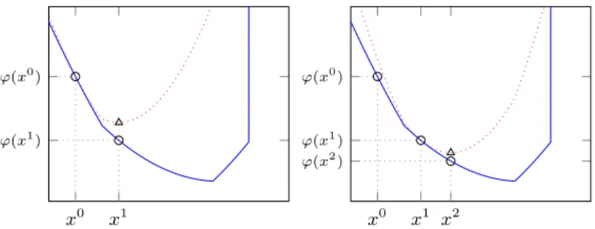
x0 x1 ϕ(x0) ϕ(x1) x0 x1 x2 ϕ(x0) ϕ(x1) ϕ(x2)
Figure 1: Whenγis small enough forward-backward splitting minimizes,
at every step, a convex majorization (red, dotted lines) of the original costϕ
(blue, solid line), cf. (2.7a).
We use shorthands to denote the forward-backward mapping and the associatedfixed-point residualin order to simplify the notation:
Tγ(x) = proxγg(x−γ∇f(x)), (2.4)
Rγ(x) =γ−1(x−Tγ(x)), (2.5)
so that iteration (2.3) can be written asxk+1 =Tγ(xk) = xk−γRγ(xk).
The setzer∂ϕis easily characterized in terms of the fixed-point set ofTγ
as follows:
x=Tγ(x)⇐⇒x∈zer∂ϕ. (2.6)
Note thatTγ(x)can alternatively be expressed as the solution to the
following partially linearized subproblem (see alsoFigure 1):
Tγ(x) = argmin u∈Rn n `ϕ(u, x) +21γku−xk2 o , (2.7a) `ϕ(u, x) =f(x) +h∇f(x), u−xi+g(u). (2.7b)
2.2
Forward-backward envelope
We now proceed to the reformulation of (2.1) as the minimization of an unconstrained continuously differentiable function. To this end, we con-sider the value function of problem (2.7a) defining the forward-backward mappingTγand give the following definition.
Definition 2.2.1(Forward-backward envelope). Letf, gandϕbe as in
As-sumption 2.1, and letγ > 0. The forward-backward envelope (FBE) ofϕwith
parameterγis ϕFBγ (x) = min u∈Rn n `ϕ(u, x) +21γku−xk2 o . (2.8)
Using (2.7a) and (2.7b) it is easy to verify that (2.8) can be equivalently expressed as
ϕFB
γ (x) =f(x) +g(Tγ(x))−γh∇f(x), Rγ(x)i +2γkRγ(x)k2 (2.9)
or, by the definition of Moreau envelope, as ϕFBγ (x) =f(x)−
γ
2k∇f(x)k
2+gγ(x
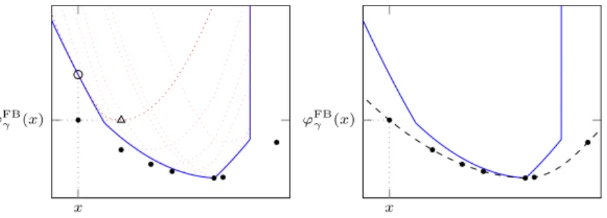
−γ∇f(x)). (2.10) The geometrical construction ofϕFB
γ is depicted in Figure 2. One
dis-tinctive feature ofϕFB
γ is the fact that it is real-valued, despite the fact
thatϕcan be extended-real-valued. Function ϕFBγ has other favorable
properties which we now summarize.
2.2.1
Basic inequalities
The following result relates the valueϕFB
γ with that ofϕ.
Proposition 2.2.2. SupposeAssumption 2.1is satisfied. ThenϕFB
γ is a strictly continuous function for anyγ >0. Moreover, for allx∈Rn
(i) ϕFBγ (x)≤ϕ(x)−γ2kRγ(x)k 2
x ϕFB γ (x) x ϕFB γ (x)
Figure 2: The forward-backward envelopeϕFB
γ (black, dashed line) is
ob-tained by considering the optimal values of problems (2.7a) (dotted lines), and serves as a real-valued lower bound for the original objectiveϕ(blue,
solid line).
(ii) ϕ(Tγ(x))≤ϕFBγ (x)− γ
2(1−γLf)kRγ(x)k
2 for allγ >0;
(iii) ϕ(Tγ(x))≤ϕFBγ (x) for allγ∈(0,1/Lf].
Proof. From the definition (2.8) and [133, Ex. 10.32], it is apparent that
ϕFB
γ is strictly continuous.
Regarding2.2.2(i), from the optimality condition for (2.7a) we have
Rγ(x)− ∇f(x)∈∂g(Tγ(x)),
i.e.,Rγ(x)− ∇f(x)is a subgradient ofgatTγ(x). From subgradient
in-equality
g(x)≥g(Tγ(x)) +hRγ(x)− ∇f(x), x−Tγ(x)i
=g(Tγ(x))−γh∇f(x), Rγ(x)i+γkRγ(x)k2.
Addingf(x)to both sides and considering (2.9) proves the claim. For
2.2.2(ii), we have
ϕFBγ (x) =f(x) +γh∇f(x), Rγ(x)i+g(Tγ(x)) +γ2kRγ(x)k2
x Tγ(x) ϕ(x) ϕ(Tγ(x)) ϕFB γ (x) x?=Tγ(x?) ϕ?
Figure 3:On the left, byProposition 2.2.2ϕFBγ (x)is upper bounded byϕ(x)
and, whenγis small enough, lower bounded byϕ(Tγ(x)). On the right, by
Proposition 2.2.3(i)the two bounds coincide in correspondence of critical points.
where the inequality follows by (2.2).2.2.2(iii)then trivially follows.
A consequence ofProposition 2.2.2is that, wheneverγis small enough, the problems of minimizingϕandϕFB
γ are equivalent.
Proposition 2.2.3. SupposeAssumption 2.1is satisfied. Then, (i) ϕ(z) =ϕFB
γ (z) for allγ >0andz∈zer∂ϕ;
(ii) infϕ= infϕFB
γ and argminϕ⊆argminϕFBγ forγ∈(0,1/Lf];
(iii) argminϕ= argminϕFB
γ for allγ∈(0,1/Lf).
Proof. 2.2.3(i)follows from (2.6),Propositions 2.2.2(i)and2.2.2(ii).
Suppose nowγ∈ (0,1/Lf]. In particular,2.2.3(i)holds for anyx? ∈
argminϕ, so
ϕFB
γ (x?) =ϕ(x?)≤ϕ(Tγ(x))≤ϕFBγ (x) for allx∈Rn
where the first inequality follows from optimality ofx? forϕ, and the
second from Proposition 2.2.2(iii). Therefore, every x? ∈ argminϕ is
also a minimizer ofϕFB
γ , andminϕ = minϕFBγ provided that the
for-mer is attained. It remains to show the caseargminϕ = ∅. By Propo-sition 2.2.2(i)we haveinfϕFB
ϕFB
γ (x) ≤infϕ, thenProposition 2.2.2(ii)implies thatϕ(Tγ(x))≤ infϕ,
contradictingargminϕ=∅. ThereforeinfϕFB
γ = infϕ, proving2.2.3(ii).
Suppose nowγ ∈(0,1/Lf), and letx? ∈argminϕFBγ . From
Proposi-tions 2.2.2(i)and2.2.2(ii)we get that
ϕFBγ (Tγ(x?))≤ϕ(Tγ(x?))≤ϕFBγ (x?)−1−γL2 fkx?−Tγ(x?)k2,
which implies x? = Tγ(x?), since x? minimizes ϕFBγ and
1−γLf
2 > 0.
Therefore, the following chain of inequalities holds ϕFBγ (x?) =ϕFBγ (Tγ(x?))≤ϕ(x?)≤ϕFBγ (x?).
SinceϕFB
γ ≤ ϕ and x? minimizes ϕFBγ , it follows that x? ∈ argminϕ.
Therefore, the sets of minimizers ofϕandϕFB
γ coincide, proving2.2.3(iii).
Example 2.2.4. To see that the bounds onγinProposition 2.2.3are tight, consider the convex problem
minimize x∈Rn ϕ(x) = f(x) 1 2kxk 2 + g(x) δRn+(x)
whereRn+ ={x∈Rn}xi≥0, i= 1. . . nis the nonnegative orthant.
As-sumption 2.1is satisfied withLf = 1, and the only stationary point forϕ
is the unique minimizerx? = 0. Using (2.10) we can explicitly compute
the FBE: for anyγ >0we have ϕFB γ (x) = 1−2γkxk 2+ 1 2γ (1−γ)x−[(1−γ)x]+ 2 ,
where[x]+= ΠR+n(x) = max{x,0}, the last expression being meant com-ponentwise. For anyγ >0we have thatϕFB
γ (x?) =ϕ(x?), as ensured by
Proposition 2.2.3(i), and as long asγ <1 = 1/Lf all properties in
Propo-sition 2.2.3do hold. Forγ= 1we have thatϕFB
γ ≡0, showing the
inclu-sion inProposition 2.2.3(ii)to be proper, yet satisfyingminϕFB
However, forγ >1the FBEϕFB
γ is not even lower bounded, as it can
be easily deduced by observing that, lettingxk= (−k,0, . . . ,0)fork∈N,
ϕFB
γ (xk) =1−2γk
2is arbitrarily negative.
Proposition 2.2.3implies, usingProposition 2.2.2(i), that anε-optimal solutionxofϕis automaticallyε-optimal forϕFB
γ and, usingProposition
2.2.2(ii), from anε-optimal solution forϕFB
γ we can directly obtain an
ε-optimal solution forϕifγ∈(0,1/Lf]:
ϕ(x)−infϕ≤ε =⇒ ϕFBγ (x)−infϕ≤ε
ϕFBγ (x)−infϕFBγ ≤ε =⇒ ϕ(Tγ(x))−infϕ≤ε.
Proposition 2.2.3also highlights the first apparent similarity between the concepts of FBE and Moreau envelope (1.11): the latter is indeed itself a lower bound for the original function, sharing with it its minimizers and minimum value. In fact, the two are directly related as we now show. In particular, the following result implies that ifϕis convex (e.g. iff is) andγ ∈(0,1/Lf), then the possibly nonconvexϕFBγ is upper and lower
bounded by convex functions.
Proposition 2.2.5. SupposeAssumption 2.1is satisfied. Then, (i) ϕFB γ ≤ϕ γ 1+γLf for allγ >0; (ii) ϕ γ 1−γLf ≤ϕFB γ for allγ∈(0,1/Lf); (iii) ϕFBγ ≤ϕγ iff is convex.
Proof. (2.2) implies the following bounds concerning the partial
lineariza-tion:
−Lf
2 ku−xk 2
≤ϕ(u)−`ϕ(u, x)≤L2fku−xk2.
Combined with the definition of the FBE, cf. (2.8), this proves2.2.5(i)and
2.2.5(ii).
Iff is convex, the lower bound can be strengthened to0 ≤ ϕ(u)−
touyields2.2.5(iii).
2.2.2
First- and second-order properties
We now turn our attention to differentiability ofϕFBγ , which is
funda-mental in devising and analyzing algorithms for solving (2.1). To ensure continuous differentiability ofϕFB
γ we will need the following
Assumption 2.3. Functionfis twice-continuously differentiable.
UnderAssumption 2.3, the function
Qγ :Rn→Rn×n given by Qγ(x) =I−γ∇2f(x) (2.11)
is well defined, continuous, and symmetric-valued. Theorem 2.2.6(Differentiability ofϕFB
γ ). Suppose thatAssumptions 2.1and 2.3are satisfied. Then,ϕFB
γ is continuously differentiable with
∇ϕFBγ (x) =Qγ(x)Rγ(x). (2.12) Ifγ∈(0,1/Lf)then the set of stationary points ofϕFBγ equalszer∂ϕ.
Proof. Consider expression (2.10) forϕFB
γ . The gradient ofgγ is given by
(1.12), and sincef ∈C2we have
∇ϕFBγ (x) =∇f(x)−γ∇2f(x)∇f(x)
+γ−1 I−γ∇2(x)
(x−γ∇f(x)−Tγ(x))
= I−γ∇2f(x)
(∇f(x)− ∇f(x) +γ−1(x−Tγ(x))).
This proves (2.12). Ifγ ∈ (0,1/Lf)then Qγ(x)is nonsingular for allx,
and therefore∇ϕFBγ (x) = 0if and only ifRγ(x) = 0, which means thatx
is a critical point ofϕby (2.6).
Together withProposition 2.2.3,Theorem 2.2.6shows that ifγ∈(0,1/Lf)
minimization of the continuously differentiable functionϕFB
γ , in the sense
that the sets of minimizers and optimal values are equal. In particular, as remarked in the next statement, ifϕis convex then the set of station-ary points ofϕFBγ turns out to be equal to the set of its minimizers, even
thoughϕFB
γ may not be convex.
Corollary 2.2.7. Suppose thatAssumptions 2.1and2.3are satisfied. Ifϕis convex (e.g. iff is), thenargminϕ= zer∇ϕFB
γ for allγ∈(0,1/Lf).
The FBE is not everywhere twice continuously differentiable in gen-eral. For example, ifgis real valued thengγ
∈C2if and only ifg
∈C2
[87]. However, second order properties will only be needed at critical points ofϕin our framework, and for this purpose we can rely on gener-alized second-order differentiability notions described in [133,§13]. Assumption 2.4. Functiongis (strictly) twice epi-differentiable atx∈zer∂ϕ
for−∇f(x), with generalized-quadratic second order epi-derivative. That is, d2g(x|−∇f(x))[d] =hd, M di+δS(d), ∀d∈Rn (2.13)
whereS ⊆ Rn is a linear subspace, andM ∈ Rn×n is symmetric, positive
semidefinite, and such thatIm(M) ⊆S andKer(M)⊇ S⊥. We refer to the case wheregis strictly twice epi-differentiable asAssumption 2.4+.
In some results we will need to assume the following slightly stronger property. The properties ofM inAssumption 2.4cause no loss of gen-erality. Indeed, lettingΠS denote the orthogonal projection ontoS (ΠS
is symmetric, see [14]), if matrixM 0 satisfies (2.13) so does matrix M0= Π
S[12(M +M>)]ΠS, which has the required properties.
Twice epi-differentiability ofgis a mild requirement, and cases where d2gis actually generalized quadratic are abundant [130,131,118,119].
For example, if g is piecewise linear and x ∈ zer∂ϕ, then from [130, Thm. 3.1] it follows that (2.13) holds if and only if the normal cone
N∂g(x)(−∇f(x))is a linear subspace, which is equivalent to
−∇f(x)∈relint∂g(x)
whererelint∂g(x)is the relative interior of the convex set∂g(x).
Example 2.2.8(Lasso). Let A ∈ Rm×n, b ∈ Rm andλ > 0. Consider f(x) =1
2kAx−bk
2andg(x) =λ
kxk1. Minimizingϕ=f+gis a frequent
problem known as lasso, and attempts to find a sparse least squares so-lution to the linear systemAx=b. One has
[∂g(x)]i= {λ} xi>0 {−λ} xi<0 [−λ, λ] xi= 0. In this cased2g(x
|−∇f(x))is generalized quadratic at a solution xas long as wheneverxi= 0it holds that|(AT(Ax−b))i| 6=λ.
We begin by investigating differentiability of the residual mapping Rγ.
Lemma 2.2.9. Suppose thatAssumptions 2.1and2.3are satisfied, and thatg
satisfiesAssumption 2.4(2.4+) at a pointx∈zer∂ϕ. Then,prox
γgis (strictly) differentiable atx−γ∇f(x), andRγis (strictly) differentiable atxwith Jacobian
JRγ(x) =γ−1(I−Pγ(x)Qγ(x)), (2.14) whereQγis as in(2.11), and
Pγ(x) =Jproxγg(x−γ∇f(x)) = ΠS[I+γM]−1ΠS. (2.15)
Moreover,Qγ(x)andPγ(x)are symmetric,Pγ(x) 0,kPγ(x)k ≤1, and if
γ∈(0,1/Lf)thenQγ(x)0.
Proof. We know from [120, Thms. 3.8, 4.1] that proxγg is (strictly)
atxfor−∇f(x). Sincef ∈C2 by assumption, then in particular
∇f is strictly differentiable. The formula (2.14) follows fromProposition 2.A.1
withP= proxγgandF(x) =x−γ∇f(x).
MatrixQγ(x)is symmetric sincef ∈ C2and positive definite ifγ < 1/Lf. To obtain an expression for Pγ(x) = Jproxγg(x−γ∇f(x))we
can apply [133, Ex. 13.45] to thetiltedfunctiong+h∇f(x), · i so that, lettingd2g = d2g(x|−∇f(x))[·]andΠ
S the idempotent and symmetric
projection matrix onS, Pγ(x)d= prox(γ/2)d2g(d) = argmin d0∈S n 1 2hd0, M d0i+ 1 2γkd0−dk 2o = ΠSargmin d0∈Rn n 1 2hΠSd0, MΠSd0i+ 1 2γkΠSd0−dk 2o = ΠS ΠS[I+γM]ΠS†ΠSd = ΠS[I+γM]−1ΠSd
where † indicates the pseudo-inverse, and last equality is due to [14,
Facts 6.4.12(i)-(ii) and 6.1.6(xxxii)] and the properties ofM as stated in Assumption 2.4. ClearlyPγ(x)0is symmetric andkPγ(x)k ≤1.
Next, we see that differentiability of the residualRγ is equivalent to
that of∇ϕFB
γ . Mild additional assumptions onf extend this kinship to
strict differentiability. Moreover, all strong (local) minimizers of the orig-inal problem,i.e., ofϕ, are also strong (local) minimizers ofϕFB
γ (and vice
versa, due to the lower-bound property ofϕFB
γ ).
Theorem 2.2.10. Suppose thatAssumptions 2.1and2.3are satisfied, and that
gsatisfiesAssumption 2.4at a pointx∈zer∂ϕ. Then,ϕFBγ is twice differen-tiable atx, with symmetric Hessian given by
∇2ϕFBγ (x) =γ−1Qγ(x)(I−Pγ(x)Qγ(x)), (2.16) whereQγandPγare as inLemma 2.2.9. If moreover∇2fis strictly continuous
atxandg satisfiesAssumption 2.4+ atx, then ϕFB
γ is strictly twice differen-tiable atx.
Proof. Recall from (2.12) that∇ϕFB
γ (x) =Qγ(x)Rγ(x). The result follows
fromLemma 2.2.9andProposition 2.A.2withQ=QγandR=Rγ.
Theorem 2.2.11. Suppose thatAssumptions 2.1and2.3are satisfied, and that
gsatisfiesAssumption 2.4at a pointx∈zer∂ϕ. Then, for allγ ∈(0,1/Lf) the following are equivalent:
(a) xis a strong local minimum forϕ; (b) for alld∈S,
d,(∇2f(x) +M)d >0;
(c) JRγ(x)is similar to a symmetric and positive definite matrix; (d) ∇2ϕFB
γ (x)0;
(e) xis a strong local