Western University Western University
Scholarship@Western
Scholarship@Western
Electronic Thesis and Dissertation Repository
9-24-2015 12:00 AM
Effects of Motion Pattern Characteristics on the Perception of
Effects of Motion Pattern Characteristics on the Perception of
Visual Acceleration
Visual Acceleration
Alexandra S. Mueller
The University of Western Ontario
Supervisor Brian Timney
The University of Western Ontario Graduate Program in Psychology
A thesis submitted in partial fulfillment of the requirements for the degree in Doctor of Philosophy
© Alexandra S. Mueller 2015
Follow this and additional works at: https://ir.lib.uwo.ca/etd
Part of the Cognition and Perception Commons
Recommended Citation Recommended Citation
Mueller, Alexandra S., "Effects of Motion Pattern Characteristics on the Perception of Visual Acceleration" (2015). Electronic Thesis and Dissertation Repository. 3331.
https://ir.lib.uwo.ca/etd/3331
This Dissertation/Thesis is brought to you for free and open access by Scholarship@Western. It has been accepted for inclusion in Electronic Thesis and Dissertation Repository by an authorized administrator of
Effects of Motion Pattern Characteristics on the Perception of Visual Acceleration (Thesis format: Monograph)
by
Alexandra S. Mueller
Graduate Program in Psychology
A thesis submitted in partial fulfillment of the requirements for the degree of
PhD in Psychology, Behavioural and Cognitive Neuroscience
The School of Graduate and Postdoctoral Studies The University of Western Ontario
London, Ontario, Canada
Abstract
The ability to perceive visual motion is one that we use every day to perform goal-directed activities, such as intercepting or avoiding objects. As objects and observers rarely move at constant velocities, it is important to be able to detect changes in velocity. However, little attention has been paid to how we perceive visual acceleration in the literature. This thesis explored the influence of real world-relevant motion pattern
characteristics on visual acceleration perception. Observers rarely see object motion with an unlimited field of view, and therefore we first examined how physically constraining the horizontal distance over which a stimulus can move affects the ability to detect and pursue horizontal acceleration and deceleration at different average velocities. Results indicated that detection improves and smooth pursuit worsens as average velocity increases. Moreover, both improve as the horizontal aperture size increases. Given our asymmetrical experience with the frequency and relevance of upward compared to downward events due to gravity, we then investigated whether acceleration and
deceleration detection vary as a function of vertical direction. We also tested whether the effects of aperture size on detection and pursuit persist on the vertical axis. Our data suggested that detection is better for downward than upward motion, and both detection and smooth pursuit improve as the vertical aperture size increases. Considering that we tend to see translation as well as more complex motion patterns outside the laboratory, we subsequently explored whether acceleration and deceleration detection vary between horizontal translation and radial optic flow, which is similar to the motion we see when moving forward or backward while looking straight ahead. We found that detection is better for radial than horizontal motion, although direction within each pattern type has no effect. Finally, we verified that sensitivity to the presence of acceleration is uniform across the optic flow field, regardless of radial direction. In summary, although we detect acceleration and deceleration similarly across a wide range of conditions, overall
perception appears to be affected by the unique characteristics of the motion pattern.
Co-authorship Statement
One manuscript has been published (Mueller & Timney, 2014a) with my co-author and PhD advisor, Dr. Brian Timney. Dr. Timney assisted with designing the experiments, analyzing and interpreting the data, and preparing all of the manuscripts for publication. All of the psychophysical experiments of this thesis were conducted in Dr. Timney’s laboratory at the University of Western Ontario, London, Ontario. Another manuscript has also been accepted pending revision for publication and two more are in preparation. Dr. Timney is a co-author on all of those manuscripts. Two of those manuscripts have three other co-authors: Drs. Esther G. González, Martin J. Steinbach, and Chris
McNorgan. Dr. González helped design and conduct the eye movement experiments. She was also instrumental for analyzing and interpreting the psychophysical and eye
movement data and she provided valuable insight on the manuscripts. The eye movement data were collected in Dr. Steinbach’s laboratory in the Vision Science Research Program at the Toronto Western Hospital, Toronto, Ontario. In addition to providing the resources for running those studies, Dr. Steinbach also gave constructive input on the two
manuscripts. During the early stages of analysis, Dr. González and I worked with Dr. McNorgan to design MATLAB programs to extract certain variables from the eye movement datasets. Although those variables were not included in this thesis, his
programming efforts were important for understanding the eye movement data and led to the analyses that were ultimately reported in the papers and in this thesis. Dr. McNorgan also gave feedback on the manuscripts.
Acknowledgements
I would first like to thank my PhD advisor, Dr. Brian Timney, for giving me the freedom and independence to pursue a wide range of projects on visual motion perception that were not necessarily the focus of his lab. I am very grateful for his continuous support and sharing his extensive knowledge about human vision and scientific writing. I am also immeasurably grateful to my mother, Dr. Esther González, as I have learned so much through my collaboration with her and Dr. Martin Steinbach. I would also like to thank Dr. Steinbach for his generosity in sharing the resources of his lab at the Toronto Western Hospital, Toronto, Ontario. Another person to whom I am greatly indebted is my father, Hans Mueller, for his technical advice on methodological design and analysis.
Thanks to Dr. Chris McNorgan for his time and patience during the MATLAB program development for the eye movement analyses and to Runjie Shi for programming the MATLAB script used to calculate peak eye velocity. I am grateful to Dr. Jody Culham for furthering my general understanding of vision science while I prepared for my PhD comprehensive exam and to Dr. Mel Goodale for his constructive insight when I needed an alternate view on how to interpret a set of results. Dr. Tutis Vilis provided me with valuable ideas for interpreting our eye movement results and Peter April answered my various technical questions about the VPixx program and rapidly addressed software issues when we discovered them. I cannot thank my participants (friends and colleagues) enough for their patience, time, effort, and perseverance. I am especially grateful to Kristie Bruinsma for her support and kindness. Without these people, none of this would have been possible. Thank you to my sister, Jennifer, for her encouragement. Finally, thank you to the examiners on my PhD defense committee: Drs. Goodale, Rob Allison, Ingrid Johnsrude, and Roy Eagleson.
I received funding for my dissertation through an Ontario Graduate Scholarship for each year of my PhD (2011 to 2015). Other sources of funding were from a Provost’s
Table of Contents
Abstract ... ii
Co-Authorship Statement ... iii
Acknowledgments ... iv
Table of Contents ...v
List of Tables ...x
List of Figures ... xi
List of Appendices ... xiv
Chapter 1 ...1
1 Introduction ...1
1.1 Acceleration Perception ...2
1.2 Ecological Influences on Acceleration Perception ...7
1.3 Vertical Acceleration Perception ...11
1.4 Acceleration Perception in Optic Flow ...12
1.5 Acceleration Versus Deceleration ...14
1.6 Summary of Experiments ...15
Chapter 2 ...19
2 General Methods ...19
2.1 General Psychophysical Method ...19
2.1.1 Participants ...19
2.1.2 Stimuli and Apparatus ...19
2.1.3 Procedure ...22
2.1.4 Analysis...24
2.2.1 Participants ...25
2.2.2. Stimuli and Apparatus ...25
2.2.3 Procedure ...26
2.2.4 Smooth Pursuit Analysis ...27
2.2.4.1 Peak eye velocity analysis ...28
2.2.4.2 Analysis of eye and stimulus position traces ...28
2.2.5 Saccade Analysis ...29
Chapter 3 ...31
3 Effects of Aperture Size and Average Velocity ...31
3.1 Experiment 1 ...32
3.1.1 Method ...32
3.1.1.1 Participants ...32
3.1.1.2. Stimuli and apparatus ...32
3.1.1.3 Procedure ...32
3.1.2 Results ...33
3.2 Experiment 2 ...34
3.2.1 Method ...35
3.2.1.1 Participants ...35
3.2.1.2 Stimuli, apparatus, and procedure ...35
3.2.2 Results ...35
3.2.2.1 Peak eye velocity ...35
3.2.2.2 Eye and stimulus position traces ...36
3.2.2.3 Saccades ...38
3.3 Discussion ...41
4 Effects of Vertical Direction and Aperture Size ...45
4.1 Experiment 3 ...46
4.1.1 Method ...46
4.1.1.1 Participants ...46
4.1.1.2 Stimuli and apparatus ...46
4.1.1.3 Procedure ...46
4.1.2 Results ...47
4.2 Experiment 4 ...48
4.2.1 Method ...48
4.2.1.1 Participants ...48
4.2.1.2 Stimuli, apparatus, and procedure ...48
4.2.2 Results ...49
4.2.2.1 Peak eye velocity ...49
4.2.2.2 Eye and stimulus position traces ...50
4.2.2.3 Saccades ...52
4.3 Discussion ...54
Chapter 5 ...57
5 Effects of Pattern Type and Direction ...57
5.1 Method ...58
5.1.1 Participants ...58
5.1.2 Stimuli and Apparatus ...58
5.1.3 Procedure ...59
5.1.4 Analysis...59
5.2 Results ...60
Chapter 6 ...64
6 Effects of Retinal Eccentricity and Radial Direction ...64
6.1 Method ...64
6.1.1 Participants ...64
6.1.2 Stimuli and Apparatus ...65
6.1.3 Procedure ...65
6.1.4 Analysis...66
6.2 Results ...66
6.3 Discussion ...67
Chapter 7 ...68
7 General Discussion ...68
7.1 Effect of the Extent of Field of View ...69
7.2 Relationship Between Smooth Pursuit and Acceleration Perception ...72
7.3 Ecological Influence of Vertical Direction ...73
7.4 Radial Optic Flow Bias ...74
7.5 Future Directions ...77
7.6 Conclusions ...78
References ...80
Appendix A ...93
Evaluating the Psychophysical Paradigm ...93
A.1 Experiment A1 ...95
A.1.1 Method ...95
A.1.1.1 Participants ...95
A.1.1.2 Stimuli and apparatus ...95
A.1.2 Results ...96
A.2 Experiment A2 ...98
A.2.1 Method ...98
A.2.1.1 Participants ...98
A.2.1.2 Stimuli and apparatus ...98
A.2.1.3 Procedure ...98
A.2.2 Results ...98
A.3 Discussion ...99
Appendix B ...101
Ethics Approval ...101
List of Tables
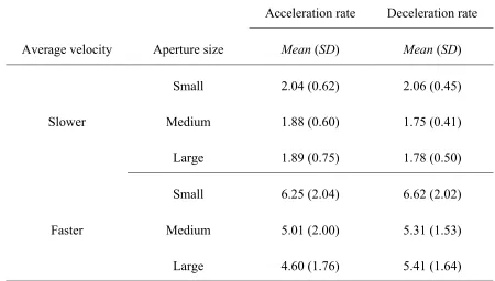
Table 1: Mean absolute 75 % correct acceleration and deceleration detection threshold rates (deg/s2) as a function of aperture size and average velocity ...33
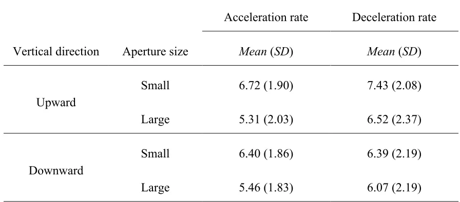
Table 2: Mean absolute 75 % correct acceleration and deceleration detection threshold rates (deg/s2) as a function of vertical direction and aperture size ...47
Table 3: Mean absolute 75 % correct acceleration and deceleration detection threshold rates (deg/s2) as a function of motion pattern direction ...60
Table 4: Mean absolute 75 % correct acceleration detection threshold rate (deg/s2) as a function of radial direction and retinal eccentricity ...66
List of Figures
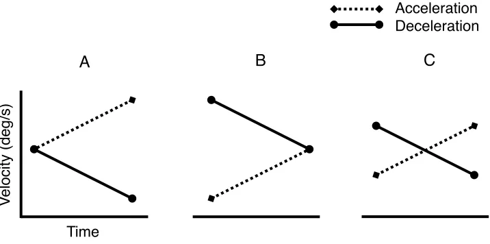
Figure 1: Schematic examples of some methods of presenting accelerating and decelerating stimuli by holding initial (A) or final (B) velocities constant or average velocity constant (C). Note that the sizes of these acceleration and deceleration rates are exaggerated for ease of visual comparison ...15
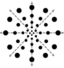
Figure 2: Schematic example of radial optic flow with dot size and density varying as a function of eccentricity from the focus of expansion. Grey dashed lines signify direction of motion ...18
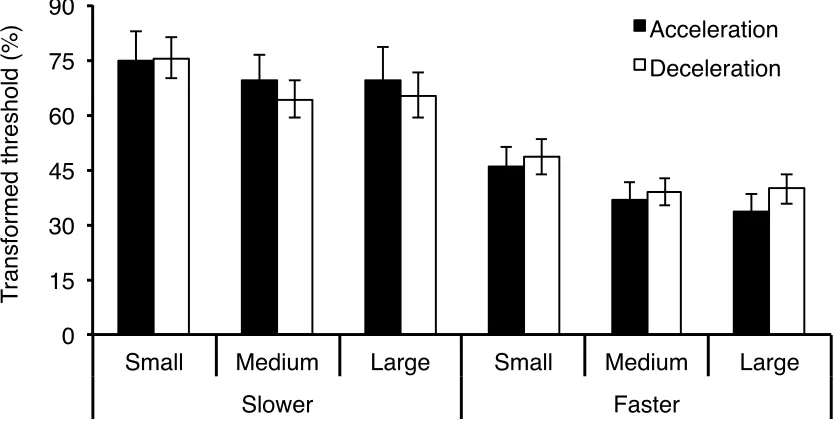
Figure 3: Mean transformed acceleration and deceleration detection thresholds (%) as a function of aperture size and average velocity. Error bars are ± 1 SE ...34
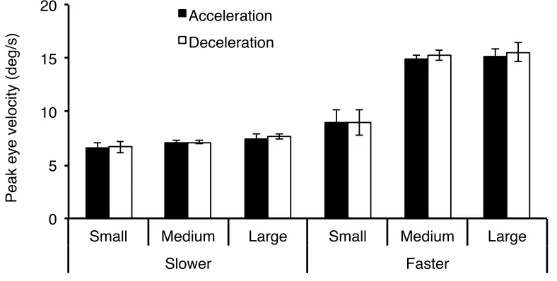
Figure 4: Mean weighted average peak eye velocity (deg/s) as a function of aperture size, average velocity, and sign of acceleration. Error bars are ± 1 SE ...35
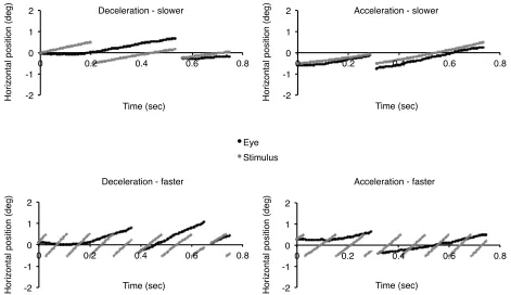
Figure 5: Example eye traces of one participant for trials belonging to the acceleration and deceleration slower and faster small aperture conditions. (Stimulus traces belong to threshold acceleration and deceleration rates, rightward motion only.) ...37
Figure 6: Example eye traces of the same participant in Figure 5 for trials belonging to the acceleration and deceleration slower and faster large aperture conditions. (Stimulus traces belong to threshold acceleration and deceleration rates, rightward motion only.) ..38
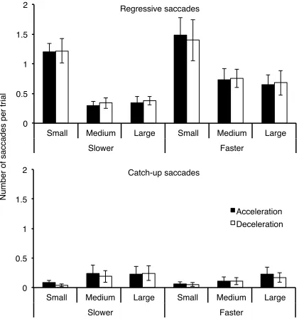
Figure 7: Mean number of regressive and catch-up saccades per trial as a function of aperture size, average velocity, and sign of acceleration. Error bars are ± 1 SE ...39
Figure 8: Mean amplitude of regressive and catch-up saccades (deg) as a function of aperture size, average velocity, and sign of acceleration. Error bars are ± 1 SE ...41
Figure 10: Mean weighted average peak eye velocity (deg/s) as a function of vertical direction, sign of acceleration, and aperture size. Error bars are ± 1 SE ...50
Figure 11: Example eye traces of one participant for trials belonging to the acceleration and deceleration upward and downward small aperture conditions. (Stimulus traces belong to threshold acceleration and deceleration rates.) ...51
Figure 12: Example eye traces of the same participant in Figure 11 for trials belonging to the acceleration and deceleration upward and downward large aperture conditions.
(Stimulus traces belong to threshold acceleration and deceleration rates.) ...52
Figure 13: Mean number of regressive and catch-up saccades per trial as a function of vertical direction, sign of acceleration, and aperture size. Error bars are ± 1 SE ...53
Figure 14: Mean amplitude of regressive and catch-up saccades (deg) as a function of vertical direction, sign of acceleration, and aperture size. Error bars are ± 1 SE ...54
Figure 15: Schematic examples of random dot pattern directions for the horizontal (on left, showing leftward and rightward directions) and radial motion conditions (on right, showing expanding and contracting directions). Direction is signified by the grey lines .59
Figure 16: Transformed acceleration and deceleration detection thresholds (%) as a function of pattern direction. Error bars are ± 1 SE ...61
Figure 17: Schematic examples of centrally and peripherally presented random dot
arrays. Grey lines signify direction for expanding and contracting motion ...65
Figure 18: Mean transformed acceleration detection thresholds (%) as a function of radial direction and retinal eccentricity. Error bars are ± 1 SE ...67
List of Appendices
Appendix A: Evaluating the Psychophysical Paradigm ...93
Chapter 1
1 Introduction
The ability to detect changes in luminance is a fundamental property of any visual system. These signals that characterize the light distribution across the retina are generally well organized and thus serve as the basis for describing changes in object position in the retinal image (Lettvin, Maturana, McCulloch, & Pitts, 1959). Moreover, the first derivative of change in position with respect to time (i.e., velocity) is an invaluable source of information for the observer to know where he or she is relative to objects in the environment. For example, motion information gives the observer the ability to accomplish goal-direct activities, such as when walking or catching a falling ball. Mechanisms that have evolved to process visual motion information range from very simple systems in insects, such as Reichardt detectors (Reichardt, 1961, 1987; Reichardt & Poggio, 1979), to very complex, multiple levels of processing in humans. In primates, the first specialized motion sensitive neurons are found in the primary visual cortex (V1), where local components of motion (i.e., temporal and spatial frequencies) are processed by neurons (i.e., complex cells) with small receptive fields (Hubel & Wiesel, 1968; Priebe, Lisberger, & Movshon, 2006; Singh, Smith, & Greenlee, 2000). In addition, there are numerous areas beyond V1 that are also involved in motion
processing, including but not limited to: V2, V3, V3A, V4, V5/middle temporal area (MT), the medial superior temporal area (MST), the fundus of superior temporal sulcus (FST), lateral intraparietal area (LIP), the ventral intraparietal area (VIP; Orban et al., 2003; Tolias, Smirnakis, Augath, Trinath, & Logothetis, 2001; Vanduffel et al., 2001), and the anterior superior temporal polysensory area (STPa; Anderson & Siegel, 1999). Furthermore, there are also several subcortical areas that have been implicated in motion processing, such as the pulvinar (Vanduffel et al., 2001), nucleus of the optic tract, and dorsal terminal nucleus of the accessory optic tract (Hoffmann & Distler, 1989).
Snowden, Treue, & Graziano, 1990; Maunsell & Van Essen, 1983; Van Essen & Gallant, 1994). In particular, although motion detectors are found in areas as early as V1, further along the visual pathway the receptive fields of these neurons increase in size and complexity, and thereby enable us to process more complex and integrated aspects of motion (e.g., form, surface, depth, and heading) in a wide range of contexts. Even so, there are parallel horizontal, feedforward, and feedback pathways that interact throughout the visual system to provide a rich perception of the world (for a review see Lamme, Supèr, & Spekreijse, 1998) and also allow for attentional modulation to enhance the perception of task-related aspects of motion in the visual image (Treue & Maunsell, 1999).
It is a complex task for the visual system to process changes in position or velocity with respect to time in the retinal image. Part of the challenge lies in the fact that the visual system must extract motion-related information from a two-dimensional retinal image of a three-dimensional world. Nevertheless, this process happens quickly (e.g., velocity discrimination performance asymptotes with stimulus presentations as brief as 150 to 200 ms, De Bruyn & Orban, 1988; Snowden & Braddick, 1991), and consequently humans are remarkably adept at perceiving visual motion. However, despite the breadth of the literature on motion perception, most studies have focused on how we perceive constant velocity and not acceleration. This is a critical gap in the literature, given that objects and observers outside the laboratory rarely move at constant velocities. For instance, when moving through the environment, people constantly speed up or slow down and make turns, automobiles regularly change their velocity, and gravity affects the motion of any object. With such variability in speed and direction, it is important to be able to detect changes to visual motion in order to accomplish voluntary goal-directed tasks, such as navigating and intercepting or avoiding objects (Braun, Schütz, & Gegenfurtner, 2010).
1.1 Acceleration Perception
the rate of acceleration directly or through comparisons of velocity over time. Prior to physiological studies on how the primate visual system processes acceleration, a number of psychophysical studies were conducted to explore how humans perceive acceleration. The ‘direct’ hypothesis holds that there are cortical neurons in the visual system that are tuned to specific rates of acceleration in the retinal image, just as there are cortical neurons that are sensitive to specific ranges of constant velocity. The ‘indirect’ hypothesis, in contrast, proposes that humans and other primates do not have cortical neurons tuned to specific acceleration rates and, instead, velocity-sensitive neurons are recruited to signal changes in velocity over time. Hypothetically, there ought to be a mechanism that uses the population responses of those neurons to detect, integrate, and evaluate velocity variations in order to detect the presence of acceleration.
We note, however, that this nomenclature of ‘direct’ and ‘indirect’ mechanisms may be misleading, given that visual motion processing does not begin immediately at the retina in primates, but further along the visual pathway in areas such as V1 and onward.
Therefore, even constant velocity is technically encoded indirectly at a cortical level because it is based on information about position-related changes from the retina. Nevertheless, the indirect hypothesis does not refer to this aspect of general motion perception. Rather, it argues that, even though constant velocity is coded explicitly at some point in the visual pathway, there may not be a mechanism that similarly codes acceleration rate in the same way. If this is the case, one may wonder how we are able to perceive acceleration at all if we do not have neurons that are sensitive to acceleration rate directly. The indirect hypothesis proposes that we have a mechanism responsible for signaling the presence of acceleration that somehow detects and integrates changes in velocity over time, but not the rate of change per se.
In general, the literature supports the indirect hypothesis. For example, Timney, Kearney, and Asa (2012) found that the ability to detect the presence of acceleration (i.e., to
stimulus’ presentation, they introduced a sudden constant velocity plateau, different acceleration rate, or deceleration rate. Hypothetically, if humans have neurons that are directly sensitive to the rate of acceleration, performance would have varied as a function of the modification of the motion profile. However, the authors found that performance was similar across conditions when the data were plotted as a function of the difference between the initial and final velocities. This suggests that an indirect mechanism is responsible for acceleration perception, and that it ‘infers’ the presence of acceleration (although this does not imply cognition) through changes in velocity over time.
Similarly, if we perceive acceleration through the rate of change in velocity directly, the duration of a stimulus’ presentation should have little effect on detection performance (Gottsdanker, Frick, & Lockard, 1961). For instance, constant velocity discrimination performance has been reported to be relatively stable after 150 to 200 ms across a wide range of base velocities (De Bruyn & Orban, 1988; Snowden & Braddick, 1991). However, if we perceive acceleration indirectly through a mechanism that relies on detecting and integrating changes in velocity over time, a longer presentation should make it easier to detect acceleration. In other words, a faster rate of acceleration should be needed for shorter presentations in order for the difference between the initial and final velocities of the stimulus to reach the threshold of an indirect mechanism that signals the presence of acceleration. In support of the latter hypothesis, Brouwer, Brenner, and Smeets (2002), Gottsdanker et al. (1961), and Timney, Solti, and Fernando (2010) demonstrated that acceleration detection improves with longer presentations (i.e., slower acceleration rates are needed for longer durations to detect acceleration reliably).
Furthermore, these authors showed that the effect of duration disappears or greatly diminishes when performance is re-plotted as a function of the relative difference between the initial and final velocities of the accelerating stimulus. These findings suggest that observers rely on the difference between the initial and final velocities to detect the presence of acceleration (at least for the brief durations tested), and we do not appear sensitive to the rate of acceleration itself.
paradigms are useful tools for investigating the mechanisms that underlie acceleration perception because acceleration is progressive changes in velocity over time. However, instead of testing a large number of contiguously presented velocities in a single stimulus presentation, these paradigms typically test only a few distinct velocities. By using fewer but discrete velocities, the researcher can manipulate the response of different groups of neurons tuned to specific velocities. For example, in many abrupt velocity change detection paradigms (e.g., Braun et al., 2010; Hohnsbein & Mateeff, 2002), a trial typically begins with a stimulus moving at a certain constant velocity and after a
specified time the stimulus abruptly increases or decreases its velocity and moves at that new velocity for a brief period, after which it returns back to its original velocity. Similar contiguous velocity presentations in velocity discrimination paradigms involve distinct velocities presented for equal durations one after the other without a temporal separation (e.g., Mateeff et al., 2000; Snowden & Braddick, 1991); in other words, the two
velocities appear sequentially within the same stimulus moving in a single direction. In comparison, most constant velocity discrimination paradigms present different velocities one after the other with a temporal separation (i.e., appearing in separate intervals).
Hypothetically, the velocities tested should elicit different responses from distinct sets of neurons tuned to ranges that overlap with those speeds and directions, regardless of whether there is a temporal separation. However, performance tends to be poorer when discriminating between contiguously presented velocities than between temporally separated velocities (Snowden & Braddick, 1991; Werkhoven, Snippe, & Toet, 1992). This suggests that the visual system may use different mechanisms to identify changes in velocity depending on whether there is a temporal separation between the distinct
velocities. In particular, the visual system may use a mechanism that infers a difference when the velocities are presented contiguously in a manner that is similar to that which has been suggested for how acceleration may be processed. This is because without the temporal separation the visual system has to rely on the combined population response of velocity detectors that varies with respect to time. Moreover, consistent with the above discussion on the effect of presentation duration on acceleration sensitivity, Gegenfurtner, Xing, Scott, and Hawken (2003) reported that contiguous velocity discrimination
second velocity to which the stimulus suddenly increases or decreases from base velocity. Although Mateeff et al. (2000) found little difference in performance between
contiguously and temporally separately presented velocity discrimination tasks for presentations longer than 500 ms and mean velocities above 8 deg/s, this most likely reflects the fact that constant acceleration is more difficult to perceive than two
contiguously presented velocities, regardless of their presentation durations (Gottsdanker et al., 1961).
The difference in how we perceive constant and variable velocity is highlighted by the general disparity in threshold performance. Weber fractions of constant velocity
discrimination thresholds tend to be extremely low, between 4 and 7 % of base velocities ranging between 4 and 64 deg/s, across a wide range of stimulus parameters (De Bruyn & Orban, 1988; Clifford, Beardsley, & Vaina, 1999; Mateeff et al, 2000; McKee, 1981; McKee & Nakayama, 1984; Orban, De Wolf, & Maes, 1984; Orban, Van Calenbergh, De Bruyn, & Maes, 1985). In comparison, Weber fractions of acceleration and abrupt
velocity change detection thresholds as well as of contiguous velocity discrimination thresholds tend to be much higher (e.g., Gottsdanker et al., 1961; Hohnsbein & Mateeff, 2002; Snowden & Braddick, 1991; Werkhoven et al., 1992). For instance, Brouwer et al. (2002) reported that a minimum 25 % difference between the initial and final velocities is necessary for observers to reliably detect the presence of acceleration, although other studies have reported Weber fractions that are much larger for acceleration detection (e.g., between 40 and 80 % in Calderone & Kaiser, 1989). Moreover, Watamaniuk and Heinen (2003) showed that, when using the same accelerating stimuli, observers perform better when asked to judge which stimulus is faster than when judging which stimulus is accelerating faster. The authors suggested that one of the reasons why the mechanism underlying acceleration perception is less sensitive than the one responsible for constant velocity perception is because it must smooth or average over local variations in the responses of the velocity detectors, which should adversely affect the visual system’s ability to register the stimulus’ acceleration rate (or even to detect that a change in velocity has occurred).
acceleration perception. Despite having cortical neurons that are sensitive to velocity, the primate visual system does not appear to have neurons that are sensitive to acceleration rate in areas that process visual motion, such as MT (Lisberger & Movshon, 1999; Price, Ono, Mustari, & Ibbotson, 2005; Schlack, Krekelberg, & Albright, 2007). Instead, the findings of these neurophysiological studies suggest that velocity tuned neurons are recruited to process changes in velocity over time. For example, a velocity detector’s response (i.e., firing rate) will increase progressively, then peak as the accelerating stimulus’ velocity passes through that neuron’s preferred velocity range, after which its response will begin to wane as the stimulus’ velocity continues beyond the preferred range—Price et al. described a typical MT neuron’s response to acceleration as inverted U-shaped. Although the signals of individual neurons do not code acceleration rate directly, their pooled population response to velocity changes over time, which is derived from their transient and sustained velocity tuning and adaptation, appears to constitute a mechanism to perceive acceleration indirectly.
In summary, the literature on acceleration perception has been largely devoted to establishing whether the underlying mechanism is direct or indirect, and the evidence is overwhelmingly in favour of an indirect mechanism. However, there are a number of other aspects of acceleration perception that have not been considered in any systematic way. One of these aspects is how the motion pattern characteristics of a stimulus affect how humans perceive visual acceleration, which was the purpose of this thesis.
1.2 Ecological Influences on Acceleration Perception
There are physical constraints on how we perceive motion in a natural environment. We do not see motion through a limitless expanse, but rather through spaces, such as
windows, spectacle frames, computer monitors, and gaps between objects. A question that arises from this is whether the physical constraints of the visual field (i.e., the aperture, or the space through which we view a moving object) influence our sensitivity to the presence of acceleration. The size of an aperture determines the distance over which an object can travel and also for how long it remains visible. Given that
2002; Gottsdanker et al., 1961; Timney et al., 2010), the longer a stimulus is able to travel uninterrupted the better the observer should be at discerning its motion profile (i.e., that the stimulus is accelerating).
Most studies that have explored the effect of aperture size on motion perception, either with respect to abrupt velocity change detection or constant velocity discrimination, have done so under fixation (e.g., De Bruyn & Orban, 1988; Hohnsbein & Mateeff, 2002; Mateeff et al., 2000). However, the length of an aperture along the axis of motion may affect an observer’s ability to track an accelerating stimulus: hypothetically, the smaller the aperture size is the more difficult it should be to track an accelerating stimulus. Moreover, it is possible is that the ability to track acceleration may influence how well we can detect the presence of acceleration.
remains on the same side of the fovea as it speeds up whereas the target will move to the other side of the fovea as it slows down. Consequently, when tracking using saccadic pursuit, larger negative velocity changes are necessary to move the target far enough to the other side of the fovea in order to create adequate retinal slip to signal that velocity is changing1. Crucially, moreover, this difference between velocity increase and decrease detection did not appear in the psychophysical performance of observers with normal smooth pursuit. In addition, performance improved with normal smooth pursuit as
compared to under fixation. Similarly, several other studies (with normal observers) have also reported that smooth pursuit improves motion sensitivity as compared to under fixation (Braun et al., 2008, Braun et al., 2010; Spering, Schütz, Braun, & Gegenfurtner, 2011; Werkhoven et al., 1992).
Although Haarmeier and Thier’s (2006) data suggest that the visual system may use retinal slip to detect changes in target velocity, their findings also indicate that there may be an optimal amount of retinal slip that is necessary for detecting velocity changes reliably. (Otherwise, systematic biases emerge that produce inaccurate motion percepts, as shown in their patient data). Therefore, it might be reasonable to expect that the size of the aperture through which the observer is able to view a stimulus accelerate should not only influence how well observers are able to track that stimulus, but also how well he or she is able to detect the presence of acceleration.
Despite the fact that this method of manipulating aperture size on the axis of motion has not been investigated with respect to acceleration perception, as mentioned above several earlier studies have examined the effects of aperture size, but they have produced mixed results. Some studies report that aperture size has little effect on velocity discrimination, except at faster velocities (256 deg/s in De Bruyn & Orban, 1988, and 32 deg/s in
Mateeff et al., 2000). In comparison, other studies have reported an effect of aperture size across a wider range of velocities. For instance, Hohnsbein and Mateeff (2002) presented
1
random dot arrays at base velocities between 8 and 32 deg/s through a rectangular aperture orientated at 0 o or 90 o, so that the distance that the dots traveled varied depending on whether the longer or shorter sides of the aperture lay on the axis of motion. They found that abrupt velocity change detection improved when the aperture was rotated to increase stimulus distance travelled, especially for velocity increases (the effect was only moderate on velocity decrease detection, although the asymmetry may have been due to differences in velocity range for each condition, as discussed in the section Acceleration vs. Deceleration below). Unfortunately for our purposes, Mateeff et al. and Hohnsbein and Mateeff presented their stimuli peripherally and under fixation, and De Bruyn and Orban presented their stimuli with durations that fell within the latency of smooth pursuit, and thus the effects observed in those studies cannot be attributed to differences in eye movements. On the other hand, Heinen and Watamaniuk (1998) found that aperture size affects smooth pursuit when tracking constant velocities, as eye
acceleration increases and latency decreases as the aperture size increases for base velocities of 4 to 8 deg/s. However, the authors manipulated the vertical height of the aperture while presenting horizontally translating stimuli, and consequently the effect of aperture size was primarily attributed to differences in the number of dots in the array (i.e., more dots in larger areas) as opposed to the area per se restricting or encouraging pursuit.
It is therefore still an open question whether the distance over which a stimulus is able to travel influences acceleration sensitivity. Although there may be a relationship between the ability to perceive and pursue acceleration depending on distance travelled, a
functional dissociation between the ocular motor and visual perceptual systems has been reported in earlier studies (e.g., Gegenfurtner et al., 2003; González, Lillakas, Greenwald, Gallie, & Steinbach, 2014; Spering & Gegenfurtner, 2007; Spering, Pomplun, &
Gegenfurtner, 2010; Tychsen & Lisberger, 1986). To further complicate the matter, there are mixed reports on whether constant acceleration perception is affected by average velocity (e.g., Brouwer et al., 2002; Calderone & Kaiser, 1989; Gottsdanker et al., 1961; Timney et al., 2010; Watamaniuk & Heinen, 2003).
The effect of average velocity on acceleration detection may vary depending on the distance over which a stimulus is able to travel. For example, motion viewed through smaller apertures appears faster than when viewed through larger apertures (Ryan & Zanker, 2001; Snowden, 1999). This effect of aperture size on apparent speed has also been shown in the Ebbinghaus–Titchener illusion (where the size of surrounding stimuli influences the perceived size of the central object). When a dot moves in a circular aperture that is surrounded by circular objects of either larger or smaller diameters, its velocity appears faster when the perceived size of the aperture is smaller (in other words, when it is surrounded by larger objects; Pavlova & Sokolov, 2000). Therefore, if the average velocity of an accelerating stimulus affects how well an observer is able to detect the presence of acceleration, it is possible that its effect on detection may vary depending on the size of the aperture.
1.3 Vertical Acceleration Perception
Many of the aforementioned studies on motion perception have used horizontal translation, however the direction of movement within the visual image may affect acceleration sensitivity because certain directions may be more behaviourally relevant than others. Due to the energy required to overcome earth’s gravitational pull, objects tend to move downward more often than they move upward in the natural world; for example, fruit growing on a tree will fall more often than it will rise into the air.
Furthermore, downward motion may be more salient to the observer than upward motion, because we tend to intercept or avoid descending objects more frequently than those traveling upward. Given our asymmetrical experience with vertical motion as a result of our daily experience with gravity, it is unclear whether we have similar anisotropies in our ability to perceive vertical acceleration.
moving upward until it reaches a vertical speed of zero, and then it accelerates downward at a constant rate. Similarly, motion duration discrimination has been reported to be more precise for downward than upward acceleration when consistent with the influence of gravity (Moscatelli & Lacquaniti, 2011). Moreover, Indovina et al. (2005) reported that the vestibular network selectively activates when the observer views acceleration that is consistent with the effects of gravity during a motion interception task (i.e., estimating when an falling object will hit a target). They suggested that this selective activation may reflect an internal model of gravity represented in the vestibular network that the visual system can recruit to help process input relating to visual acceleration. Expectations about the way gravity affects the vertical acceleration and deceleration of objects manifest early in life (Kim & Spelke, 1992), and the downward bias in positive acceleration sensitivity has been attributed to an experience-based adaptation in the human visual system (Moscatelli & Lacquaniti, 2011). However, it remains to be demonstrated whether we have a bias to perceive deceleration in the opposite direction.
Alternatively, Hecht, Kaiser, and Banks (1996) reported that observers rely on average velocity, as opposed to acceleration rate, to judge the distance traveled of objects in free fall. Similarly, Senot, Prévost, and McIntyre (2003) found that observers use online information about velocity, and not acceleration rate, to estimate time-to-contact for intercepting accelerating objects. Consequently, if we are relatively insensitive to acceleration on the vertical axis, perhaps vertical direction affects acceleration and deceleration detection similarly. Therefore, one might expect a general downward bias in acceleration and deceleration perception. Furthermore, if the area over which one can track improves sensitivity, there may be an interaction between vertical direction and aperture size on acceleration and deceleration detection. In other words, a difference in acceleration and deceleration sensitivity (if one exists) as a function of vertical direction may change depending on the size of the aperture.
1.4 Acceleration Perception in Optic Flow
plane, where all of the dots in the array move leftward or rightward) instead of more visually complex motion patterns. Although we do experience translation when we move our heads laterally or when tracking objects moving across our visual field, we also tend to see more complex forms of motion when we move through the environment because we live in a three-dimensional world. In consideration of Gibson’s (1979) ecological approach to understanding visual perception, we may be ‘wired’ in some fashion to perceive motion better in certain kinds of stimuli than in others. Specifically, the more visually complex and realistic stimuli are, the more representative psychophysical performance should be in a laboratory setting. One type of motion pattern that meets these criteria is radial optic flow because as we move through the environment, or when objects move relative to us, we typically see visual patterns of radial optic flow.
Moreover, radial optic flow is more visually complex than translation because there is simultaneous cardinal and oblique motion throughout the display. Nevertheless, it remains to be shown whether there is a difference in how we detect the presence of acceleration in radial optic flow patterns as compared to in horizontal translation patterns. Studies that have investigated the effect of motion pattern type on motion perception in general (although not with respect to visual acceleration perception) have produced conflicting results (e.g., Bex & Makous, 1997; Bex, Metha, & Makous, 1998; Edwards & Badcock, 1993; Edwards & Ibbotson, 2007; Freeman & Harris, 1992; Lee & Lu, 2010).
Even though direction of optic flow informs the observer about his or her motion relative to the environment, a critical point of information about heading comes from the focus of optic flow. In particular, heading discrimination has been reported to be better when optic flow is presented in the centre of the visual field than in the periphery as well as when the focus of optic flow is near the fovea (Warren & Kurtz, 1992). Similarly, although
Crowell and Banks (1993) observed that heading sensitivity is more affected by the eccentricity of the focus of optic flow than where the optic flow field is located on the retina, they too reported that sensitivity is higher when the focus of optic flow is near the fovea. This in turn raises the question of whether observers rely more on the centre of the optic flow field than the periphery to detect the presence of acceleration.
1.5 Acceleration Versus Deceleration
A feature of acceleration is that it can be positive or negative. Although one might
Figure 1. Schematic examples of some methods of presenting accelerating and decelerating stimuli by holding initial (A) or final (B) velocities constant or average velocity constant (C). Note that the sizes of these acceleration and deceleration rates are exaggerated for ease of visual comparison.
1.6 Summary of Experiments
One of the goals of this thesis was to explore how the ability to detect the presence of acceleration is affected by physically constraining the distance over which a random dot stimulus can travel. We did this by manipulating the size of the aperture on the axis of the stimulus’ motion. In particular, we varied the aperture’s horizontal distance for
horizontally accelerating and decelerating stimuli in Experiment 1 and its vertical height for vertically accelerating and decelerating stimuli in Experiment 3. We hypothesized that larger apertures would encourage smooth pursuit and improve acceleration and
deceleration detection, whereas smaller fields would restrict smooth pursuit and worsen detection. To test whether the size of the aperture does affect the ability to track, we conducted control experiments in which we measured the effects of aperture size on smooth pursuit on the horizontal and vertical axes in Experiments 2 and 4, respectively.
Due to the mixed reports of an effect of average velocity on acceleration sensitivity, we had no hypotheses as to whether acceleration and deceleration sensitivity would improve as average velocity increases, although we anticipated that smooth pursuit should worsen
Acceleration!
Deceleration!
V
e
lo
ci
ty
(d
e
g
/s)
!
Time!
as average velocity increases. Nevertheless, we expected that sensitivity and smooth pursuit should improve as the size of the aperture increases, regardless of average velocity. Using horizontal translation, in Experiments 1 and 2 we manipulated the average velocity of the acceleration and deceleration conditions for various horizontal aperture distances. Experiment 1 measured acceleration and deceleration detection accuracy, and Experiment 2 was a control experiment designed to determine whether the aperture size manipulation varies how observers pursue acceleration and deceleration as a function of average velocity.
In Experiment 3, using vertically translating random dot stimuli, we tested two alternative hypotheses with respect to the effects of vertical direction and sign of acceleration on acceleration detection as a function of vertical aperture height. First, it is possible that the visual system is sensitive to the effects of gravity and thereby also to the sign of
acceleration as a function of vertical direction. If this is the case, we should detect downward acceleration and upward deceleration better than upward acceleration and downward deceleration. On the other hand, such a degree of sensitivity needed to distinguish between vertical acceleration and deceleration may be an inefficient use of resources, considering that we do not appear to be particularly sensitive to the rate of acceleration in the first place. The second hypothesis holds that the downward bias in detection persists regardless of the sign of acceleration. Both hypotheses are consistent with the idea of an experience-based adaptation and each would predict acceleration and deceleration detection to improve as the area over which one is able to pursue the moving stimuli increases. If the ability to detect acceleration and deceleration is better over larger than smaller areas, the effect of aperture size may alter the strength of the asymmetry (if it exists) between the acceleration and deceleration conditions as a function of vertical direction. Experiment 3 measured the effects of vertical direction, aperture size, and sign of acceleration on acceleration detection accuracy. Experiment 4 was a control
experiment to test whether the height of the vertical aperture varies smooth pursuit of vertical acceleration and deceleration.
Figure 2. Schematic example of radial optic flow with dot size and density varying as a function of eccentricity from the focus of expansion. Grey dashed lines signify direction of motion.
Chapter 2
2 General Methods
There are two types of studies reported in this thesis: psychophysical and eye tracking. The experiments within each category used the same general methodology. In this chapter, the general psychophysical methodology is outlined first, followed by the general eye tracking methodology. Each of the subsequent chapters that describe an individual experiment includes a Method section with the methodological particulars.
2.1 General Psychophysical Method
Experiments 1, 3, 5, and 6 (in Chapters 3, 4, 5, and 6 respectively) tested acceleration detection accuracy with a two-interval forced choice (2IFC) task using the
psychophysical method of constant stimuli. These experiments were conducted at the University of Western Ontario, London, Ontario, in accordance with the guidelines and regulations of the university’s Research Ethics Board. Participants volunteered or were reimbursed up to $40 for travel expenses in Experiments 1 and 3, and they were paid $20 in Experiment 5 and $10 in Experiment 6.
2.1.1 Participants
All participants had normal or corrected–to–normal visual acuity and stereoacuity with no known visual or ocular motor disorders (e.g., strabismus or amblyopia) and no history of eye muscle surgery or patching. Visual acuity and stereoacuity were measured using a Master Ortho-Rater (Bausch and Lomb, Rochester, NY), and stereoacuity was further assessed using the Randot® StereoTest (Stereo Optical Co., Inc., Chicago, IL). Participants wore their normal optical correction if necessary.
2.1.2 Stimuli and Apparatus
pixel was 0.001 o). The stimuli were continuously (and 100 % coherently) moving
random dot arrays of white dots (96.7 cd/m2) on a black background (0.06 cd/m2) through a simulated, invisible stationary aperture (i.e., the border of the aperture was not visibly defined and dots disappeared when they left the aperture area). Dot position was updated every frame and dot lifetime was unlimited. Dot size, average density, and
velocity/acceleration/deceleration were constant across the aperture in every condition within an experiment, although the dot parameters varied between experiments. Every aperture through which the random dot arrays were presented was centered in the middle of the screen. Aperture size and shape were specific to each experiment.
Two types of motion patterns (on a 2-D surface) were tested in this thesis: translation (horizontal and vertical) and radial optic flow (expansion and contraction). At the start of every stimulus’ presentation, a set of dots was generated and placed at (average)
uniformly distributed random positions in the frame. Within each subsequent frame, the dots were displaced by the same amount, which corresponded to the stimulus’ speed divided by the frame rate. For the horizontally (Experiments 1, 2, and 5) or vertically moving stimuli (Experiments 3 and 4), all of the dots moved in the same direction. For the expanding or contracting stimuli, the direction of displacement depended on the dot location in the stimulus; specifically, dots were displaced in a direction along the vector from the centre (or periphery) of the stimulus to their current position. This resulted in all of the dots streaming outward (for expansion) or inward (for contraction) from the centre of the display; however, there were no spatial speed or density gradients in the arrays. Every dot’s speed increased or decreased over the course of the presentation according to the acceleration rate for that particular trial.
dot density in order to keep average dot density uniform in every frame. Specifically, the VPixx program partitioned the optic flow field into eight uniformly spaced eccentricities and eight uniformly spaced meridians (resulting in 45 o intervals). This produced 64 truncated annuli that were centred on the focus of expansion/contraction, which was located in the centre of the display. For a given frame, VPixx calculated the instantaneous dot density within each of these annuli and then calculated a low-pass filtered time-averaged density that was equal to half of the instantaneous density plus half of the previous frame’s time-averaged density. Whenever a dot reached the border of the aperture, it was replaced by a new one at a random location within the truncated annulus that had the lowest time-averaged density. Several earlier studies have used similar radial motion stimuli (e.g., Morrone et al., 2000; Smith, Wall, Williams, & Singh, 2006; Wall & Smith, 2008). These methods of presenting radial and horizontal motion meant that each individual frame was indistinguishable between the horizontal and radial motion stimuli.
Every experiment (including the eye movement experiments) presented both acceleration and deceleration, with the exception of Experiment 6, which only presented acceleration. Regardless of the sign of acceleration presented, the motion profile of every dot was calculated using the following formula:
𝑣𝑒𝑙𝑜𝑐𝑖𝑡𝑦= 𝑣!"##$% + 𝑎∗ 𝑡− 𝑡!"#$%&'(
2 , (1)
accelerating or decelerating based on the distance travelled within each trial, which was essential for our manipulation of aperture size. In addition, the initial and final velocities of an array were constant for a given rate of acceleration across aperture sizes within each velocity range tested.
2.1.3 Procedure
Every psychophysical experiment used a 2IFC task with the method of constant stimuli, in which there were 7 rates of acceleration and deceleration for the comparison stimuli for each condition (with the exception of Experiment 6, which only tested positive acceleration). A standard stimulus (constant velocity) and a comparison stimulus
(acceleration/deceleration) were presented in random order in every trial. The task was to detect which stimulus was accelerating/decelerating.
Participants were always tested in the dark and viewed the screen binocularly from a distance of 60 cm, using a chin rest to minimize head movements. At the beginning of every trial a red fixation target with the shape of a 0.5 o diameter crosshair against a black background was presented for 500 ms. We chose this fixation target shape because Thaler, Schütz, Goodale, and Gegenfurtner (2013) reported it to be the most effective in producing stable fixation. To control initial eye position participants were told to fixate the crosshair target at the beginning of every trial until the random dot stimuli were presented (during which they were free to move their eyes), with the exception of Experiment 6 where participants were told to keep fixating the centre of the screen even after the fixation target had disappeared. The fixation target then disappeared and was followed immediately by either the standard or comparison stimulus for 750 ms, followed by a black screen for 500 ms, and then the standard or comparison stimulus for another 750 ms. Participants were asked to identify whether the first or the second display accelerated (or decelerated) and they indicated their decision by pressing a key on a keyboard. Trials were self-paced, initiated by pressing the spacebar. An audible beep followed all key and spacebar presses.
runs were blocked further according to experimental condition. The order of the acceleration and deceleration blocks was counterbalanced across participants. In Experiment 5, acceleration and deceleration were randomly interlaced across trials. Experiment 6 only presented accelerating stimuli. The order of the conditions and the stimulus values within each condition were always randomized in every experiment. In Experiments 1 and 3, direction within each condition (aperture size by average velocity in Experiment 1, and aperture size in Experiment 3) was randomized. In Experiments 5 and 6, direction was blocked into separate conditions. Direction was analyzed in Experiments 3, 5, and 6, but not in Experiment 1. Participants always completed one condition at a time.
Participants were given practice trials prior to beginning the experimental task, and the minimum number of practice trials varied between experiments. Every psychophysical experiment had a minimum number of 20 experimental trials per stimulus value per condition (with the exception of Experiment A2 in Appendix A which had a minimum of 10 trials). However, the maximum number of experimental trials per stimulus value included for each condition varied because it was based on the number of trial runs needed to obtain psychometric functions with non-significant Pearson Chi-square coefficients of goodness of fit per participant, as described below. The only exception to this was Experiment 5. All observers reported that the task in Experiment 5 with
2.1.4 Analysis
SPSS Statistics software (IBM Corporation, Armonk, NY) was used to analyze the data. The number of correct responses for each stimulus value within each condition was plotted in terms of proportion correct as a function of acceleration or deceleration rate. Probit regression was used to get psychometric functions with non-significant Pearson coefficients of goodness of fit (as determined through Chi-square analyses) and to interpolate the 75 % correct threshold acceleration/deceleration rate for each condition.
In order to compare performance in the psychophysical experiments of this thesis to that of earlier studies, the absolute 75 % correct detection threshold rates were transformed into values that were functionally equivalent to Weber fractions. We could not transform the thresholds using the acceleration rates directly because the standard stimulus was always a pattern moving at constant velocity and therefore with an acceleration rate of zero. Using the standard equation to calculate the Weber fraction (ΔA/A) would result in a denominator of zero and so the fraction could not be calculated. Instead, we performed a linear transformation to express the acceleration threshold rate in terms of the
difference between the minimum and the maximum velocities (vmin and vmax) divided by the velocity of the standard stimulus (i.e., the average velocity of the accelerating or decelerating stimulus). In other words, the transformed thresholds represent the threshold percent difference between the maximum and minimum velocities of the comparison stimulus relative to the velocity of the standard stimulus needed to detect the presence of acceleration or deceleration. This method of transforming acceleration detection
thresholds has been reported before (e.g., Brouwer et al., 2002; Calderone & Kaiser, 1989; Gottsdanker et al., 1961). We used the following equation:
𝑡𝑟𝑎𝑛𝑠𝑓𝑜𝑟𝑚𝑒𝑑𝑡ℎ𝑟𝑒𝑠ℎ𝑜𝑙𝑑= 𝑣!"#− 𝑣!"#
𝑣!"#+ 𝑣!"#
2
100. (2)
0.05. Although the transformed thresholds were of primary interest, in every
psychophysical experiment the mean absolute 75 % correct acceleration and deceleration detection threshold rates are presented in tables. We note that statistical analyses revealed the same results for the absolute and transformed threshold datasets because the
transformation was linear. The only exception to this was Experiment 1, which tested different average velocities and therefore large differences in absolute thresholds were to be expected (as discussed in Chapter 3).
2.2 General Eye Tracking Method
The purpose of the eye tracking experiments in this thesis was to serve as a control to test whether the ability to pursue an accelerating or decelerating random dot array varies depending on the aperture size on the horizontal and vertical axes. Experiments 2 and 4 investigated smooth pursuit using a single stimulus presentation method. Both
experiments were conducted at the Toronto Western Hospital, Toronto, Ontario, in accordance with the guidelines and regulations of the University of Western Ontario and the University Health Network’s Research Ethics Boards. The data from Experiments 2 and 4 were collected during the same testing session. The order of experiments was counterbalanced across participants. Participants were reimbursed for travel expenses up to $40.
2.2.1 Participants
Five volunteers (including author ASM) participated in both Experiments 2 (horizontal eye movements) and 4 (vertical eye movements), having also previously participated in the psychophysical Experiments 1 (horizontal motion) and 3 (vertical motion). These five individuals had an average age of 25.6 years (SD = 1.52) and four were female.
2.2.2 Stimuli and Apparatus
(version 2.87) on a 45 cm Samsung monitor (Sync Master 900 NF; Samsung, Seoul, South Korea), with a 120-Hz refresh rate and 1024 x 768 pixel resolution. The MacBook Pro laptop used to run the VPixx program was connected to a desktop remote video-based EyeLink 1000 eyetracker (SR Research Ltd., Mississauga, Ontario, Canada) through the eye tracker’s host computer using a DATAPixx interface (VPixx
Technologies Inc., Saint-Bruno, Quebec, Canada). The DATAPixx interface recorded time and stimulus condition information in the data files. Eye position was recorded with the eye tracker with a sampling rate of 250-Hz. The eye tracker was calibrated for every participant prior to the experimental task using its software’s standard calibration and validation procedures.
2.2.3 Procedure
Participants were tested at a 60 cm viewing distance in an illuminated room, viewing binocularly, and sitting with their head (chin and forehead) resting against a headrest. A single motion stimulus was presented in every trial. Trials were initiated automatically and began with a red 0.5 o diameter crosshair fixation target on a black background for 1000 ms, followed immediately by an accelerating or decelerating stimulus presented for 750 ms. Another trial followed immediately. The participants were instructed to fixate the crosshair target at the beginning of every trial and then to track the moving stimulus and try to determine if the motion was accelerating or decelerating (in order to keep
participants focused on the task), however no verbal or key press responses were required. Acceleration and deceleration trials were randomly presented within each condition. Order of conditions (aperture size by average velocity in Experiment 2, and aperture size in Experiment 4) and direction within each condition was randomized. There were 10 trials for each stimulus value per condition. Participants completed one condition at a time.
The stimulus values used in Experiments 2 and 4 were based on the absolute 75 % correct detection threshold rates in Experiments 1 and 3, respectively. Three values were used for each condition in each eye movement experiment. The first stimulus value was the
threshold rate obtained in the corresponding condition in the psychophysical experiment. The second and third rates were 50 % and 100 % greater than the 75 % correct detection threshold rate, respectively, in order to have a range of stimulus values to measure observers’ smooth pursuit in response to acceleration and deceleration. The three stimulus values tested in every condition were unique to each participant. We note, moreover, that smooth pursuit performance was similar between the three rates tested within each condition for Experiments 2 and 4.
2.2.4 Smooth Pursuit Analysis
The eye movement data were analyzed offline, and saccades, fixations, and blinks were removed from the data prior to analysis of smooth pursuit. Saccades were identified using the standard EyeLink saccade detection algorithm, with a combined criterion of eye velocity > 22 deg/sec and eye acceleration > 4000 deg/sec2 (saccades were analyzed separately from the smooth pursuit data). In the event of a blink, the data corresponding to 100 ms before and 100 ms after the initial occlusion of the pupil were removed (Aguilar & Castet, 2011).
We analyzed smooth pursuit in terms of peak eye velocity and eye position traces. The reason why we analyzed peak eye velocity, despite having presented continuously
accelerating stimuli, is because data are lost through the filtering process used to calculate the second derivative (which is also susceptible to noise). Moreover, the aim of using the measure of peak velocity is to see whether it varies as a function of experimental
traces allowed us to understand the peak velocity data. An advantage with investigating eye position with respect to time is that, because the eye tracker records eye position over time, this method has no data loss. Furthermore, by plotting the traces of eye position against stimulus position, we obtained interesting results with respect to eye trajectory and location within the visual field, which would not have been evident if we had only analyzed peak eye velocity. Only eye movements (of the right eye) made in the direction of the stimulus motion are reported.
2.2.4.1 Peak eye velocity analysis. Peak velocity of the right eye during epochs of uninterrupted smooth pursuit was calculated using a custom MATLAB (MATLAB, Mathworks, Natick, MA) script that used a 5-point differentiator. The program
approximated the first derivative of eye position with respect to time (i.e., eye velocity) through the 5-point stencil method (Equation 3, where x is eye position and h is the spacing between eye positions):
𝑓! 𝑥 = −𝑓 𝑥+2ℎ +8𝑓 𝑥+ℎ −8𝑓 𝑥−ℎ +𝑓 𝑥−2ℎ
12ℎ . (3)
First we calculated the peak eye velocity for every uninterrupted epoch of smooth pursuit. Then, we created a weighted average of all of the peak velocities (taking into account the number of data points that contributed to each peak velocity value) that occurred for a particular stimulus value within an experimental condition. (Recall that there were three stimulus values, i.e., acceleration or deceleration rates, per condition.) Finally, we averaged those weighted average values in order to obtain a measure of mean weighted average peak eye velocity for each condition per participant. We submitted the mean weighted average peak eye velocities to repeated measures ANOVAs, using the
Greenhouse-Geisser correction if necessary and the Holms-Bonferroni correction with α at 0.05 for all pairwise comparisons. As an aside, although one might wonder whether these data reflect the maximum velocities of the stimuli tested, the peak eye velocities reported in Experiments 2 and 4 are much higher than any of the peak stimulus velocities.
Therefore, after obtaining the stimulus velocities for every time point using Equation 1, we calculated stimulus position using Equation 42:
𝑝𝑜𝑠𝑖𝑡𝑖𝑜𝑛!!! = 𝑝𝑜𝑠𝑖𝑡𝑖𝑜𝑛! + 𝑣𝑒𝑙𝑜𝑐𝑖𝑡𝑦! 𝑡!!!−𝑡! . (4)
We set the initial position of the stimulus to the initial position of the right eye at the beginning of every epoch of uninterrupted smooth pursuit, because all of the dots within the array accelerated or decelerated at the same rate across the visual field. For the cases in which the initial eye position occurred outside the area of the aperture, we set the stimulus’ initial position at the boundary of the aperture closest to the initial eye position in order to keep the stimulus motion restricted to the aperture area. Whenever the
stimulus reached the edge of the aperture in the direction of motion, it was reset to the opposite side of the aperture for the subsequent time point. This reset method for the instances in which smooth pursuit was interrupted by either a saccade or a blink avoids the issue of stimulus positions depending on the number and accuracy of saccades. Examples of this analysis are shown in Experiments 2 and 4.
2.2.5 Saccade Analysis
In addition to smooth pursuit eye movements, we also explored saccadic eye movements (of the right eye only). There were two types of saccades: regressive saccades (in the opposite direction of stimulus motion) and catch-up saccades (in the direction of stimulus motion). Prior to analysis, we removed all the saccades that occurred during the pre and post-100 ms of the initiation of a blink as well as during the first 200 ms of the stimulus presentation; that is, during initiation of pursuit from fixation (Krauzlis, 2004; Lisberger,
2 The eye tracker sampled at 250-Hz whereas the CRT monitor refreshed at 120-Hz. Given that
Chapter 3
3 Effects of Aperture Size and Average Velocity
Experiment 1 was designed to investigate whether physically constraining the distance over which a stimulus can travel influences the ability to perceive acceleration. We anticipated that the distance traveled should also affect how well the observer is able to track the moving stimulus (Experiment 2), which in turn should be related to the effect of aperture size on psychophysical performance because there are reports that smooth pursuit can improve motion sensitivity (e.g., Braun et al., 2008; Braun et al. 2010; Haarmeier & Thier, 2006; Spering, Schütz, et al., 2011; Werkhoven et al., 1992). In the present series of experiments we manipulated distance traveled by varying the horizontal extent of the aperture through which we presented horizontally accelerating and
decelerating random dot arrays, and we also explored the effect of average velocity on acceleration sensitivity. In Experiment 1 we measured acceleration and deceleration detection accuracy as a function of aperture size and average velocity. Experiment 2 was a control experiment to determine whether the size of the aperture varies how well observers can track accelerating and decelerating stimuli as a function of velocity.
We hypothesized that acceleration and deceleration detection would improve as the size of the aperture increases at both slower and faster average velocities in Experiment 1. Although Hohnsbein and Mateeff (2002) reported that abrupt velocity change detection improves as velocity increases, studies on constant acceleration perception, such as Brouwer et al. (2002), have reported mixed findings for the effect of velocity depending on the task and whether thresholds are reported as absolute or relative (i.e., Δv
final-initial/vaverage). Although we expected large differences in absolute thresholds between the