A Pattern Synthesis Method for Large Planar Antenna Array
Youji Cong*, Guonian Wang, and Zhengdong Qi
Abstract—The pattern synthesis for large antenna arrays is very important because of its wide applications. Several antenna array synthesis techniques for planar antenna array have been developed in the past years. In this paper, a hybrid method for solving antenna array pattern synthesis problem is introduced. The proposed method has three steps. Firstly, the iterative fast Fourier transforms (IFT) is used to generate a number of initial array excitations based on aim pattern. Then, the global optimization method differential evolution strategy (DES) is used to optimize these excitations based on initial excitations. After that, if the optimized pattern does not satisfy the goal, the simulated annealing (SA) method is applied to optimize the excitations until the goal is achieved or the maximum iteration is reached. Several simulation results show that the desired pattern can be effectively synthesized by using the proposed method.
1. INTRODUCTION
In recent years, antenna array has attracted more and more attention, because it has a wide range of applications in radar, mobile communications, and other electronic systems. These electronic systems need various antenna patterns due to complex engineering applications. So pattern synthesis is urgently required, especially in large antenna arrays. However, the synthesis of antenna arrays to generate an aim radiation pattern is a highly nonlinear optimization problem.
Nowadays, various synthesis methods have been proposed, but they have some limitations. Classical method such as Dolph-Chebyshev [1] and Taylor-Kaiser [2] can obtain analytical element excitations instantly, but only for synthesizing simple patterns, such as low side lobe pencil beam. Some complicated pattern can be synthesized by Woodward-Lawson [3] quickly, however this method can only be used in linear array. As the pattern synthesis problem is an optimization issue, convex optimization (CVX) [4, 5, 28] method is applied. The CVX can quickly find the optimization solution of objective function. However it will be helpless when solving large antenna array synthesis. General optimization methods such as the steepest descent or conjugate gradient [26], they are usually slow converging and easy to fall into local optimal solution. In 1990s, the global optimization methods, such as the genetic algorithm (GA) [6, 7], particle swarm optimization (PSO) [8–10], differential evolution Strategy (DES) [11–13], and Simulated Annealing (SA) [14, 15] are presented. They all simulate evolutionary phenomena of nature to find the optimization solution. These methods have the capability of performing better and more flexible solutions than the classical optimization methods and the conventional analytical approaches. However, challenges still exist. The computation cost is so huge that the time will not be tolerated when solving synthesis problems for large antenna arrays.
Recently, the iterative fast Fourier transforms (IFT) [16, 17] was proposed to synthesize the large antenna arrays with uniform grid spacing. The inverses Fourier transform relationship between the array factor and the element excitation distribution is used in this algorithm. As a version of the alternating projection techniques [18–20, 27], the IFT derives the element excitations from the array factor using
Received 25 July 2015, Accepted 2 September 2015, Scheduled 4 September 2015
* Corresponding author: Youji Cong ([email protected]).
successive forward and backward Fourier transforms. As fast Fourier transforms (FFT) technique is applied, the array pattern and excitation distribution are obtained rapidly by several iterations, and this algorism is very suitable for solving large antenna array synthesis problems. But it will not get good results when the aim antenna pattern is very complex, the iteration will stop ahead frequently.
In this paper, a hybrid synthesis algorithm is proposed, which is based on the IFT and artificial intelligent algorithm DES and SA. As IFT can obtain the array excitation quickly, the initial population for DES is generated by IFT. Then the cell excitation is optimized by DES which has high calculation efficiency. After that SA is applied for optimizing the solution generating by DES. In this way, the disadvantages of IFT can be avoided and the optimization efficiency increases. In this paper, the effect of mutual coupling between antenna elements is also considered. The simulation results show that the method we proposed is effective and accurate when solving the large antenna array synthesis problems. The paper is organized as follows. In Section 2, the details of the method will be discussed. Several synthesis examples will be presented in Section 3. The last section of the paper is the conclusion.
2. FORMULATIONS AND ALGORITHMS 2.1. Problems Formulation
The far-field pattern of an array antenna is calculated by the formula (1) [21]
F F(θ, ϕ) =EP(θ, ϕ)×AF(θ, ϕ) (1)
whereAF(θ, ϕ) is the array factor (AF), andEP(θ, ϕ) represents the active element pattern of phased arrays [22]. EP(θ, ϕ) can be obtained by testing or electromagnetic simulation. For a 2-D planar antenna array,AF(θ, ϕ) can be calculated by formula as follows.
AF(θ, ϕ) =
M
m=1 N
n=1
Imnexp
i2π
λ (xmnsin(θ) cos(ϕ) +ymnsin(θ) sin(ϕ))
(2)
whereλis the wavelength, andImn,xmn andymn are the complex excitation and position of themnth antenna element, respectively.
For a typical antenna synthesis problem, the magnitude of far-field pattern|F F(θ, φ)| is required to be close to the target pattern, or between the boundaries of the limitation patterns, such as
|F Fmin(θ, φ)| ≤ |F F(θ, φ)| ≤ |F Fmax(θ, φ)|, where|F Fmin(θ, φ)|and|F Fmax(θ, φ)|are the corresponding
desired lower and upper bounds on the antenna pattern, respectively. A good fitness function to be minimized is defined as
F itness=
I
i=1 J
j=1
(|F Fobj(θij, ϕij)−F F(θij, ϕij)|)2 (3)
whereF Fobj(θij, ϕij) andF F(θij, ϕij) are the objective and optimized far-field pattern value evaluated at far-field angles θij and ϕij, respectively.
The complex excitationImnwill also be required in some specific issues. For example, the excitation amplitude dynamic range often requires less than a certain value. And in some times, the only-phase synthesis is required. In this paper, our goal is to obtain a complex excitation Imn which can generate the objective antenna pattern calculated by formula (1) and (2).
2.2. Iterative Fourier Technique (IFT)
The IFT technique starts with the calculation of far-field pattern P0, using an initial excitation
distributionE0 which has M×N elements. The K×K point (K = 2n >2·max(M, N)) 2-D inverse
FFT is applied to calculate the far field pattern. The bigger the K value, the more accurate the far-field pattern, but the computation time will be longer. Then the P0 region beyond the request boundary
part is corrected while the other keeps the same. After this correction, a direct K-point 2-D FFT is performed on the modified AF to get an updated set of the excitation coefficients. From the K×K excitation coefficients, onlyM×N samples belonging to the array are retained as new excitation, while the others are forced to zero. The new excitation will be also corrected if the amplitude or the phase does not satisfy the request. After the correction, the updated excitationE0, and a new updated pattern P0 are gotten. The iteration will be repeated until the new updated pattern and excitation satisfy the
requirements or the max iterate number is achieved.
The implementation of the IFT algorithm for synthesis of a required pattern for 2-D planar arrays in this paper involves the steps as follows:
(1) Generate twoM×N matrixes A and P as the amplitude and phase for element excitation randomly, the matrix elements of A are fixed or within a setting dynamic range, the matrix elements of P are random ranges −180◦ ∼+180◦, so the initial complex excitation E0 isA·exp(i·π·P/180).
(2) Compute AF based on initial complex excitation E0 using a K×K−point inverse FFT, with K= 2n>2·max(M, N), and the far-field patternP0 is calculated by formula (1).
(3) Adapt theP0 to the described pattern, substituting the described pattern forP0 whose part exceeds
the boundary of the limitation patterns. Next, the array factor AF is obtained by dividing updated
P0 by the active element pattern.
(4) Compute the updated excitation E0 for the adapted AF by using the K × K −point direct
FFT. Extract the amplitude A and phase P of E0 by the
real(E0)2+imag(E0)2 and
arctan(imag(E0)/real(E0)) respectively.
(5) Modify the complex excitationE0 to meet the set range,and the updated complex excitation E0 is
gotten.
(6) Repeat the steps (2)∼(5), until the prescribed far-field pattern is satisfied, or the allowed number of iteration is reached.
The IFT can be easily and efficiently implemented in the pattern synthesis problem, especially for the large antenna array which has more than 1000 element numbers. This method is also flexible to deal with complex antenna patterns or excitation constraints synthesis problems by a little change of steps (3) and (5).
2.3. Differential Evolution Strategy (DES)
The DES has its origin of the Vector Difference idea by Ken Price when he was solving the Chebyshev polynomial fitting problem [23]. This idea is modified and improved by Storn and Price for several times, and ultimately form the DES. The steps of the classical DES are as follows [24]:
(1) GenerateN initial population V, here the V represents the complex excitation.
(2) Mutate the initial farms by differential mutation operator, and a new variation vector for each optimization vector is generated. The differential mutation operator has the form as
VM,i=V(n),opt+β·(V(n),p1−V(n),p2) p1, p2 ∈(1, . . . , N), p1=p2=i, i= 1, . . . , N
(4)
where N is the population size, V(n),opt is the best individual of father farm, and the mutation factor β is a constant which can be used to control the differential magnification. The amplitude of complex excitation are modified to meet the setting range.
(3) The cross operation. V(n),i and its corresponding mutation individual have the crossover operation
at a certain probability, generating offspringVC,i,
(VC,i)j =
(VM,i)j, γ < pcross
(V(n),i)j, γ≥pcross (5)
(4) The choice of operation. The offspring individuals produced by crossover operator and parent individuals are compared. If the fitness of offspring individuals is less than the parent individuals, the offspring individuals replace the parent individuals; otherwise the parent individuals will remain in the next generation.
(5) The termination operation. The operation will be stopped when the best individual of progeny population has reached the optimization goal or the max iteration number is achieved, otherwise repeat the steps (2)∼(5).
The DES has the advantage of simple operation, fast optimization speed, and excellent searching ability. However it will be convergence stagnation and even premature convergence in some engineering problems.
2.4. The Simulated Annealing Algorithm (SA)
The SA is a kind of general probabilistic algorithm, which is introduced by S. Kirkpatrick et al. [25]. The basic idea of the SA is similar to the behavior of a material in the cooling process. According to the theory, the value of objective function at every state within the searching space can be treated as the “energy” of a fictitious material. Then an energy function with respect to the fictitious material will be minimized. Here the fitness function is treated as the energy function, which is defined as formula (3) with respect to complex excitations. The key idea is to find the optimized excitations. When the SA is implemented, the maximum temperature T0, the maximal iteration number K, and the excitation
variable are all initialized. The fitness function can be calculated quickly by formula (1) ∼ (3) using FFT. The SA algorithm has several parts: cooling procedure, and the inner iteration. The cooling procedure contains cooling rate and the stop threshold. Here the cooling temperature is defined as
Tn=T0·rn, wherer is the cooling rate. The cooling procedure stops as the temperature Tn is lower
than defined lowest temperature. At one temperature, each iteration of the SA algorithm starts with an antenna excitation configuration Eold, and the new stateEnew is gotten by randomly changes the state of Eold. If the new stateEnew cause the value of fitness function decrease, it is accepted. Otherwise it is accepted in a probability P in a current temperature. The accepted probability P is calculated by formula (6)
P(Ebest=Enew) =
1 if Δf < o
exp(−Δf/Tn) if Δf ≥0 (6)
where Δf =F itness(Enew)−F itness(Eold). From formula (6), we can find that the higher temperature, the higher accepted probability of the new solution as Δf ≥0. To update the new state Enew is very important for the key potential of global optimization due to non-linear problem. In this paper, a simple and effective algorithm is implemented as follows
Enew =Eold+ ΔE (7)
where ΔEis the additive excitation matrix which has the adding amplitude and phase of the excitation. The amplitude of complex excitation are modified to meet the setting range. Here the number and the position of the adding excitation elements are given beforehand and randomly respectively. By the formula (7), the solutions around the current optimization solution are exploited.
The SA procedure stops until the temperature is lower down to the minimum. And the optimization excitation is obtained after the SA procedure.
2.5. Hybrid Pattern Synthesis Method
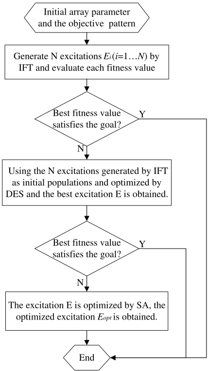
In this paper, a hybrid pattern synthesis method is proposed. Three different basic optimization ideas are applied here, which are the IFT, DES, and SA. Owing to the respective defect and advantages of IFT, DES and SA, three optimization methods are combined in this paper. The overall procedure is summarized in the flow chart of Figure 1.
Generate N excitations Ei(i=1…N) by IFT and evaluate each fitness value
Best fitness value satisfies the goal? Initial array parameter and the objective pattern
Using the N excitations generated by IFT as initial populations and optimized by DES and the best excitation E is obtained.
Best fitness value satisfies the goal?
The excitation E is optimized by SA, the optimized excitation Eopt is obtained.
End N N
Y Y
Figure 1. Flow chart of the proposed hybrid approach.
is too spare to describe the details. However when K is too large, the calculation speed is so slow that the synthesis efficiency will be reduced. Generally, K is set to be 256 or 512. A judgment is used to determine whether to continue the optimization process.
If the best value of the fitness function generated by IFT does not satisfy the goal, the DES is implemented for its advantage of fast convergence speed and good searching ability. However, convergence stagnation often happens in the DES process. The optimized parameters β and Pcross in the DES are very important, which can affect the final optimization result. In general, β is between 0.55 and 0.7 while Pcross is set in arrange [0, 1] respectively. In this paper, optimized parameters are carefully set and adjusted depending on the different issues.
After the DES optimization process, a best excitation is gotten. Thereafter the SA algorithm starts when the solution is not good either. The SA has a slower convergence speed, but the excellent searching ability. In the SA process, we have some steps such as repeating heating to enhance the searching ability. The iteration stops when value of the fitness function is satisfied or the max number iteration is reached.
3. SYNTHESIS EXAMPLE
Several pattern synthesis simulations are performed here to illustrate the accuracy and efficiency of the proposed method. The simulations employ two examples. One is the cosecant beam synthesis for a linear array which has 16 antenna elements, the results of synthesis method and full wave method are compared. The other is the flat-top beam synthesis for a large planar array which has more than 3000 antenna elements.
3.1. Cosecant Beam Synthesis for a Linear Array
A 45 degree cosecant beam synthesis for a 16 linear waveguide array showing in Figure 2 is presented. This example is to demonstrate the accuracy of the proposed method.
In this case, the active element pattern in the array is considered in pattern synthesis. The excitation amplitude and phase are all employed in the pattern synthesis, and the excitation amplitude dynamic range ratio (DRR) is set to below 1.85. Some main parameters of synthesis method are as follows, the max IFT iteration number is 100; the DES population size is 40, and the iteration number is 40, the mutation factor beta is 0.5, and the cross probability Pcross is 0.95; the maximum iteration steps for SA is 500.
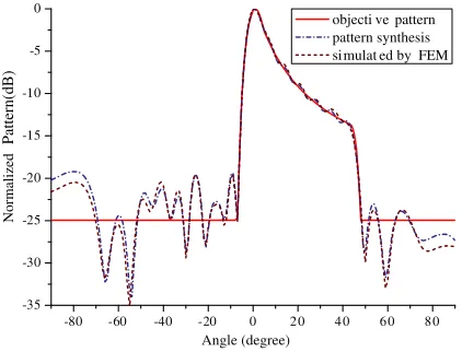
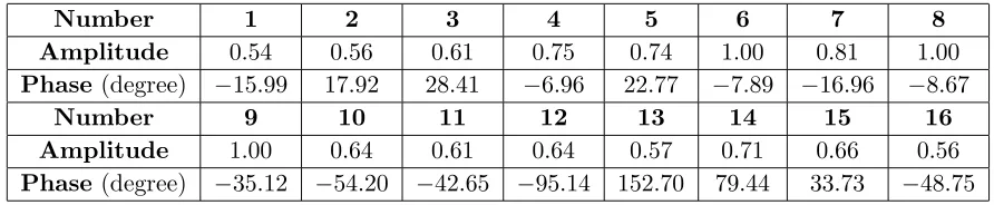
Figure 3 shows the synthesis result. The optimized pattern is in agreement with the full wave simulation results. The tiny difference is caused by the neglect of the small differences between the active element patterns in the array. Figure 4 shows the synthesis pattern without employing the active element pattern,which deviates from the full wave simulated result. Table 1 and Table 2 give the amplitude and phase values of two cases respectively. The active element pattern is a key factor in the pattern synthesis especially for the wide shaped beam. In practice, if the array is large enough, considering only the middle element pattern can meet the precision requirement.
Figure 2. A 16 linear waveguide array for 45 degree cosecant beam synthesis.
-80 -60 -40 -20 0 2 0 4 0 6 0 8 0
-35 -30 -25 -20 -15 -10 -5 0
Normalized
Pattern(dB)
Angle (degree)
objecti ve pattern pattern synthesis simulat ed by FEM
Figure 3. Synthesis result of cosecant beam. In the optimization process, the influence of the active element pattern is considered.
-80 -60 -40 -20 0 2 0 4 0 6 0 8 0
-35 -30 -25 -20 -15 -10 -5 0
Normalized Pattern (dB)
Angle (degree)
objective pattern pattern synthesis simulat ed by FEM
Table 1. Synthesised excitation amplitude and phase of the waveguide linear array (with active element pattern).
Number 1 2 3 4 5 6 7 8
Amplitude 0.54 0.98 0.86 0.61 0.54 0.65 1.00 0.91 Phase (degree) 42.64 −36.17 −119.15 140.89 58.50 70.62 37.85 18.10
Number 9 10 11 12 13 14 15 16
Amplitude 1.00 1.00 0.83 0.81 0.62 0.54 0.54 0.54 Phase (degree) 21.07 0.67 3.24 −3.06 −15.09 −1.58 −32.95 24.25
Table 2. Synthesised excitation amplitude and phase of the waveguide linear array (without active element pattern).
Number 1 2 3 4 5 6 7 8
Amplitude 0.54 0.56 0.61 0.75 0.74 1.00 0.81 1.00 Phase (degree) −15.99 17.92 28.41 −6.96 22.77 −7.89 −16.96 −8.67
Number 9 10 11 12 13 14 15 16
Amplitude 1.00 0.64 0.61 0.64 0.57 0.71 0.66 0.56 Phase (degree) −35.12 −54.20 −42.65 −95.14 152.70 79.44 33.73 −48.75
3.2. Flat-Top Beam Synthesis
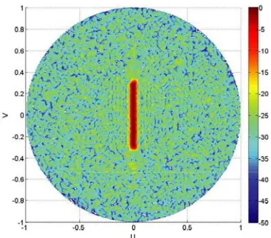
Flat-top beam is commonly used in engineering. In this case, pattern synthesis bases on a large scale array which has more than 3000 elements containing 60 rows, 60 columns. The radiation elements are triangular arrangement, and the line spacing is 0.5 wavelengths while the column spacing is 0.5 wavelengths too. The goal 3 dB beam width of flat-top beam is 32 deg, about 20 times the pencil beam broadening, while the ripple is below 1 dB. In this case, only the phase is optimized, so the excitation amplitude is set all the same.
For this synthesis problem, the active element pattern here is assumed to be cos(θ). Some main parameters settings are as follows, the max IFT iteration number is 100; the DES population size is 40, the iteration number is 40, the mutation factor β is 0.45, and the cross probability Pcross is 0.95; the maximum iteration steps for SA is 360. The FFT calculate point is 256×256.
Figure 5 and 6 show the simulation results. The ripple of the flat-top is less than 1 dB, and the side lobe is less than−22 dB. In order to demonstrate the features of this method, several synthesis methods such as IFT alone, IFT combined with DES, DES combined with SA are compared here. The above numerical methods are all computed on a PC with Intel i3-2100 3.1 GHz CPU. The average convergence curves of 50 trials are shown in Figure 7. Table 3 gives the average synthesis trial time of different methods.
Table 3. Optimization time of different synthesis method.
Synthesis method IFT+DES+SA IFT alone IFT+DES DES+SA
Optimization time 328s 17s 448s 253s
Figure 5. Relative power patterns of flat-top beam synthesis.
-80 -60 -40 -20 0 2 0 4 0 6 0 8 0
-50 -40 -30 -20 -10 0
Normalized Pattern
Angle (degree)
Figure 6. Section of synthesised flat-top beam.
0 100 20 0 300 40 0 500
10 100
Fitness Value
Iteration Number
IFT+DES+SA IFT IFT+DES DES+SA
Figure 7. Convergence curves of several synthesis methods.
4. CONCLUSIONS
In this paper, a hybrid pattern synthesis method for large antenna array is proposed. The IFT and artificial intelligent algorithm DES, SA are the bases of the algorithm. The method starts with the excitations generated by IFT, and then the excitations are optimized by DES and SA. FFT algorithm is implemented here to accelerate the pattern calculation. The coupling effect of the antenna elements has also been considered in the synthesis process, so optimized pattern is more close to the actual application. Several simulations illustrate the efficient and accuracy feature of the method. In practice, different combination methods can be chosen according to different problems.
ACKNOWLEDGMENT
REFERENCES
1. Elliot, R. S., Antenna Theory and Design, Prentice-Hall, Englewood Cliffs, NJ, 1981. 2. Constantine A. Balanis, Antenna Theory, Wiley, New York, 1997.
3. Durr, M., A. Trastoy, and F. Ares, “Multiple-pattern linear antenna arrays with single prefixed distributions: Modified Woodward-Lawson synthesis,”Electron. Lett., Vol. 26, 1345–1346, 2000. 4. Li, M., Y. Chang, Y. Li, J. Dong, and X. Wang, “Optimization polarized pattern synthesis of
wideband arrays via convex optimization,” IET Microw. Antennas Propag., Vol. 7, No. 15, 1228– 1237, 2013.
5. Fuchs, B., “Application of convex relaxation to array synthesis problems,”IEEE Trans. Antennas Propagat., Vol. 62, No. 2, 634–640, Feb. 2014.
6. Yan, K. K. and Y. Lu, “Sidelobe reduction in array-pattern synthesis using genetic algorithm,”
IEEE Trans. Antennas Propagat., Vol. 45, No. 7, 1117–1122, Jul. 1997.
7. Mahanti, G. K., A. Chakraborty, and S. Das, “Phase-only and amplitude-phase only synthesis of dual-beam pattern linear antenna arrays using floating-point genetic algorithms,” Progress In Electromagnetics Research, Vol. 68, 247–259, 2007.
8. Bevelacqua, P. J. and C. A. Balanis, “Minimum sidelobe levels for linear arrays,” IEEE Trans. Antenna Propagat., Vol. 55, No. 12, 2210–2217, Dec. 2007.
9. Recioui, A., “Sidelobe level reduction in linear array pattern synthesis using particle swarm optimization,” Jour. of Optimization Theory and Applic., Vol. 153, 497–512, 2012.
10. Khodier, M. M. and C. G. Christodoulou, “Linear array geometry synthesis with minimum sidelobe level and null control using particle swarm optimization,”IEEE Trans. Antennas Propagat., Vol. 53, No. 8, 2674–2679, Aug. 2005.
11. Yang, S., Y. B. Gan, and A. Qing, “Sideband suppression in time-modulated linear arrays by the differential evolution algorithm,” IEEE Antennas and Wireless Propagation Letters, Vol. 2002, No. 1, 173–175, 2002.
12. Rainer, S. and K. Price, “Differential evolution — A simple and efficient heuristic for global optimization over continuous spaces,”J. of Global Optimization, Vol. 4, 341–359, 1997.
13. Yikai, C., et al., “The application of a modified differential evolution strategy to some array pattern synthesis problems,”IEEE Trans. Antennas Propag., Vol. 56, 1919–1927, 2008.
14. Trucco, A., “Thinning and weighting of large planar arrays by simulated annealing,”IEEE Trans. Ultrason., Ferroelect., Freq. Control, Vol. 46, No. 2, 347–355, Mar. 1999.
15. Trucco, A., E. Omodei, and P. Repetto, “Synthesis of sparse planar arrays,”Electron. Lett., Vol. 33, No. 22, 1834–1835, Oct. 1997.
16. Keizer, W. P. M. N., “Fast low-sidelobe synthesis for large planar array antennas utilizing successive fast Fourier transforms of the array factor,” IEEE Trans. Antennas Propagat., Vol. 55, No. 3, 715– 722, Mar. 2007.
17. Keizer, W. P. M. N., “Low-sidelobe pattern synthesis using iterative fourier techniques coded in MATLAB,” IEEE Antennas and Propagation Magazine, Vol. 51, No. 2, 137–150, Apr. 2009. 18. Bucci, O. M., G. Franceschetti, G. Mazzarella, and G. Panariello, “Intersection approach to array
pattern synthesis,”IEE Proc.-Pt. H, Vol. 137, No. 6, 349–357, Dec. 1990.
19. Bucci, O. M., G. D’Elia, G. Mazzarella, and G. Panariello, “Antenna pattern synthesis: A new general approach,” Proc. IEEE, Vol. 82, No. 3, 358–371, Mar. 1994.
20. Quijano, J. L. A. and G. Vecchi, “Alternating adaptive projections in antenna synthesis,” IEEE Trans. Antennas Propag., Vol. 58, No. 3, 727–737, Mar. 2010.
21. Li, W. T., X.-W. Shi, and Y.-Q. Hei, “An improved particle swarm optimization algorithm for pattern synthesis of phased arrays,”Progress In Electromagnetics Research, Vol. 82, 319–332, 2008. 22. Pozar, D. M., “The active element pattern,” IEEE Trans. Antennas Propagat., Vol. 42, No. 8,
1176–1178, Aug. 1994.
24. Chen, Y., S. Yang, and Z. Nie, “The application of a modified differential evolution strategy to some array pattern synthesis problems,”IEEE Trans. Antennas Propag., Vol. 56, No. 7, 1919–1927, 2008.
25. Liu, J., Z. Zhao, K. Yang, and Q. H. Liu, “A hybrid optimization for pattern synthesis of large antenna arrays,”Progress In Electromagnetics Research, Vol. 145, 81–91, 2014.
26. Fong, T. S. and R. A. Birgenheier, “Method of conjugate gradients for antenna pattern synthesis,”
Radio Sci., Vol. 6, 1123–1130, 1971.
27. Franceschetti, G., et al., “Array synthesis with excitation constraints,” IEE Proceedings H: Microwaves, Antennas and Propagation, Vol. 135, No. 6, 400–407, 1988.