Estimation of Flexible Pavement Structural Capacity Using Machine Learning Techniques

(1)

1

Estimation of Flexible Pavement Structural Capacity Using Machine Learning Techniques

Running title:

Estimation of Flexible Pavement Structural Capacity Using ML Techniques

Nader KARBALLAEEZADEHa_{, Hosein GHASEMZADEH TEHRANI}b*_{, Danial MOHAMMADZADEH} S.c,d_{, Shahaboddin SHAMSHIRBAND}e,f*

a_{Civil Engineering Department, Shahrood University of Technology, Shahrood, Iran} b_{Civil Engineering Department, Shahrood University of Technology, Shahrood, Iran} c_{Department of Civil Engineering, Ferdowsi University of Mashhad, Mashhad, Iran}

d_{Department of Elite Relations with Industries, Khorasan Construction Engineering Organization, Mashhad}

9185816744, Iran

e _{Department for Management of Science and Technology Development, Ton Duc Thang University, Ho Chi}

Minh City, Vietnam

f _{Faculty of Information Technology, Ton Duc Thang University, Ho Chi Minh City, Vietnam}

* _{Corresponding author. E-mail: [email protected], [email protected]}

Abstract

The most common index for representing structural condition of the pavement is the structural number. The current procedure for determining structural numbers involves utilizing falling weight deflectometer and ground-penetrating radar tests, recording pavement surface deflections, and analyzing recorded deflections by back-calculation manners. This procedure has two drawbacks: 1. falling weight deflectometer and ground-penetrating radar are expensive tests, 2. back-calculation ways has some inherent shortcomings compared to exact methods as they adopt a trial and error approach. In this study, three machine learning methods entitled Gaussian process regression, m5p model tree, and random forest used for the prediction of structural numbers in flexible pavements. Dataset of this paper is related to 759 flexible pavement sections at Semnan and Khuzestan provinces in Iran and includes “structural number” as output and “surface deflections and surface temperature” as inputs. The accuracy of results was examined based on three criteria of R, MAE, and RMSE. Among the methods employed in this paper, random forest is the most accurate as it yields the best values for above criteria (R=0.841, MAE=0.592, and RMSE=0.760). The proposed method does not require to use ground penetrating radar test, which in turn reduce costs and work difficulty. Using machine learning methods instead of back-calculation improves the back-calculation process quality and accuracy.

Keywords transportation infrastructure, flexible pavement, structural number prediction, Gaussian process regression, m5p model tree, random forest

1 Introduction

As the service life of pavement begins, various distresses debilitate its structural capacity. Structural capacity plays a vital role in identifying damaged pavements and choosing maintenance treatments[1]. The pavement engineers seek strategies to maintain pavement quality at an acceptable level. Thus, it is essential to implement a pavement management system (PMS)[2]. Although considerations related to pavement structural condition have not been taken into account in many PMSs, many agencies and institutes have incorporated structural indices in PMS and the making-decision process in recent years[3]. For pavement engineers, it is essential to know the future structural condition of pavement[4]. Thus, the prediction of pavement performance is one of the critical steps of PMS. In PMS, performance prediction models employed for the following purposes[5]:

• To predict the future condition of the pavement

• To optimize, prioritize, schedule and determine the type of maintenance treatments

• To analyze the effect of treatments on pavement future condition

• To estimate the life cycle costs for different maintenance scenarios

• To examine the feedbacks of pavement design processes

(2)

2

The estimation of pavement future performance and evaluation of its results can contribute to maintaining and elongating the pavement service life[6, 7]. Evaluation tests for pavements classified into two major categories[8]: 1. Destructive Testing (DT), 2. Non-Destructive Testing (NDT). The DTs have several disadvantages, such as coring the asphalt, Interfering with the traffic flow, and requiring a long implementation time[7]. Unlike DTs, application of NDTs has gained momentum in recent years because they allow accurate simulation of real conditions, which is not feasible under laboratory conditions. Considering its possibility of in-site simulation, NDT reduces both costs and time[6, 7]. The most common NDT equipment used to evaluate both flexible and rigid pavements is falling weight Deflectometer (FWD) [7, 9]. In the FWD test, a loading plate and a series of geophones are placed on the surface of pavement, and exposed to 40 KN axle load over a period of 25 to 35 milliseconds. Geophones measures surface deflections of pavement and send them to a central computer for analysis. Using various software such as ELMOD and MODULUS, this central computer provides valuable information like structural number (SN), remaining service life (RSL), and overlay thickness (DOL) [4, 10-12]. For completing the analysis process in the central computer of FWD, layers thickness information is essential. Pavement layer thickness determined by another NDT called ground penetrating radar (GPR). GPR transmits electromagnetic waves to the pavement structure and then reports layers thickness as a continuous profile along the road [10, 13].

The structural capacity of pavement defined as its ability to bear the traffic load without excessive distresses[6]. The primary index for the structural capacity of pavement is SN. The relationship between SN and pavement structure defined according to Eq. (1) [14]:

𝑆𝑁 = (𝑎1𝐷1+ 𝑎2𝑚2𝐷2+ 𝑎3𝑚3𝐷3) (1)

where a1 is asphalt layer coefficient; a2 is base layer coefficient; a3 is subbase layer coefficient; m2 is base drainage coefficient; m3 is subbase drainage coefficient; D1 is asphalt thickness (inch); D2 is base thickness (inch), and D3 is subbase thickness (inch).

SN is a positive number that the highest value of it is at the beginning of pavement life. The initial structural capacity of a new pavement decreases by passing the traffic flow. Therefore, engineers use “SNeff” phrase when they evaluate the pavement for the selection of maintenance treatments. Effective structural number (SNeff) is the effective SN of the pavement, which represents pavement strength at the time of evaluation. As mentioned above, the most practical way to determine SNeff is to carry out the FWD test. The current method to determine the SNeff suffers from two significant drawbacks: 1. It is necessary to perform a surplus NDT, called GPR, to determine the pavement layers thickness, 2. Data analysis performed by back-calculation methods, which are inherently ambiguous and inaccurate.

Given that the utilization of machine learning (ML) for solving the nonlinear problems has become very popular in the past years[15], this paper first tries to fix the mentioned problem about the data analysis method in the prior paragraph. For this purpose, the authors used three ML techniques, including Gaussian process regression (GPR), m5p model tree (M5P) and random forest (RF), to estimate SNeff. The other problem mentioned in the former paragraph is related to an excess test called GPR. For solving this problem, the authors utilized the surface deflections and surface temperature of the pavement as inputs in modeling. As such, there is no need for GPR test.

(3)

3

The employment of pavement surface temperature is the main innovation in this paper because no researchers have adopted this variable as input in their modeling up to now. Another innovation is related to using ML techniques. All other researchers have analyzed the data using basic statistical methods and have used statistical software such as SPSS and SAS.

This paper is organized as follows: Section 2 presents a literature review. Section 3 introduces the study methodology. Section 3 has three subsections including NDTs, ML, and performance metrics. The results are presented and discussed in Section 4. Finally, Section 5 offers a summary of the results and conclusions of the paper.

2 Literature review

In general, there are two approaches to pavement performance prediction [5, 16]: deterministic and probabilistic approaches. In the former, for each set of input variables values, a single value is predicted as the pavement performance. The latter is generally carried out in three procedures [17]:

• Mechanistic

• Empirical

• Mechanistic-Empirical (M-E)

The deterministic approach has two primary shortcomings [18, 19]:

• Disability in demonstrating input data dispersion and application of mean values.

• Over-design and under-design problems generated by the adoption of reliability coefficients.

On the contrary, a probabilistic approach predicts the pavement performance based on the probability of occurrence. The main probabilistic methods are [5]: Machine learning, Markov probability matrices, survivor curves, and Bayesian inference techniques.

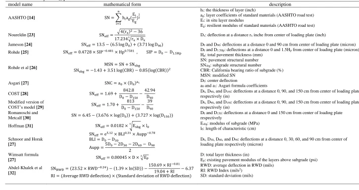
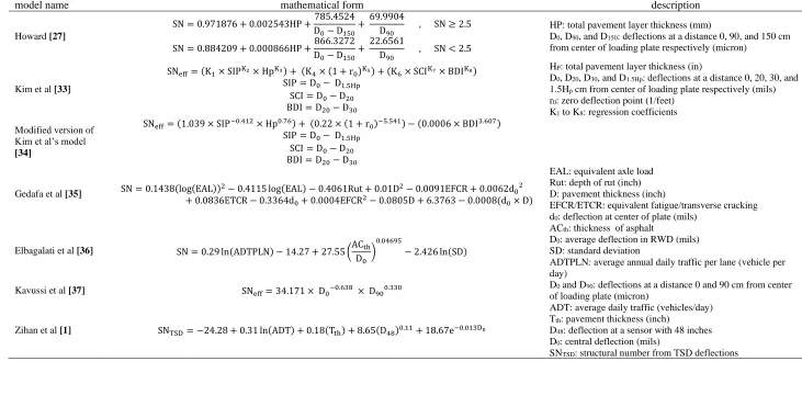
ML is a soft computing technique widely utilized to develop the performance models of pavement [20, 21]. Contrary to the common perception, ML techniques do not act as a black box but rather as statistical training methods. Many ML techniques are used to model pavement performance, including artificial neural networks (ANN) and support vector regression (SVR) [5, 22]. In the above techniques, the machine seeks to detect the intercommunication of outputs and inputs by taking biases and weights into account [5]. The performance of an in-service pavement determined by the introduction and calculation of an index. There are several indices for pavement performance, such as Pavement Condition Index (PCI), Riding Number (RN), International Roughness Index (IRI), Present Serviceability Index (PSI), and SNeff. SNeff is a numerical index that reflects the structural status and the bearable traffic load of an existing pavement. Prediction of SNeff has been the subject of growing scholarly attention and numerous papers addressed this subject. The most prominent SNeff prediction models presented in Table 1.

Significant results and lessons learned from this table are:

1. By review of Table 1, the first point to be made clear is that the base of SN prediction models is surface deflections. Therefore, the authors used surface deflections as the primary input in modeling.

(4)

4

Table 1 Summary of SNeff prediction models

1

model name mathematical form description

AASHTO [14] SN = ∑ hiag(

Ei Eg )13 n

i=1

hi: the thickness of layer (inch)

ag: layer coefficients of standard materials (AASHTO road test)

Ei: in situ layer modulus

Eg: resilient modulus of standard materials (AASHTO road test)

Noureldin [23] SNeff=

√4(rx)2− 36 17.234√r3 x× Dx

Dx: deflection at a distance rx inche from center of loading plate (inch)

Jameson [24] SNeff= 13.5 − (6.5 log D0) + (3.71 log D90) D0 and D90: deflections at a distance 0 and 90 cm from center of loading plate (micron)

Rohde [25] SNeff= 0.4728 × SIP−0.481× Hp0.7581 , SIP = D0− D1.5Hp D_H0 and D1.5Hp: deflections at a distance 0 and 1.5Hp from center of loading plate (micron)

p: total pavement thickness (mm)

Rohde et al [26] MSN = SN + SNsbg

SNsbg= −1.43 + 3.51 log(CBR) − 0.85(log(CBR))2

SN: pavement structural number SNsbg: subgrade structural number

CBR: California bearing ratio of subgrade (%) MSN: modified SN

Asgari [27] SNC = a0× (D0)a1 D

0: center deflection

a0 and a1: Asgari formula coefficients

COST [28] SNeff= 1.69 +

842.8 D0− D150

− 42.94 D90

D0, D90, and D150: deflections at a distance 0, 90, and 150 cm from center of loading plate

respectively (in) Modified version of

COST’s model [29] SNeff= 1.70 +

813 D0− D150

− 39 D90

D0, D90, and D150: deflections at a distance 0, 90, and 150 cm from center of loading plate

respectively (in) Romanoschi and

Metcalf [30] SN = 6.45 − (3.676 × log(D0)) + (3.727 × log(D150))

D0 and D150: deflections at a distance 0 and 150 cm from center of loading plate

respectively

Hoffman [31] SNeff= 0.0182 × √Esbg

3

× l0 E_lsbg: modulus of subgrade (MPa)

0: length of characteristic (cm)

Schnoor and Horak [27]

SNeff= e5.12× BLI0.31× Aupp−0.78 BLI = D0− D30

Aupp =5D0− 2D30− 2D60− D90 2

D0, D30, D60, and D90: deflections at a distance 0, 30, 60, and 90 cm from center of

loading plate respectively (micron)

Wimsatt formula

[27] SNeff= 0.00045 × D × √E3 P

D: total layer thickness (in)

Ep: existing pavement modulus of the layers above subgrade (psi)

Abdel-Khalek et al [32]

SNRWD= (23.52 × RWD−0.24) − (1.39 × ln(SD)) −

150.69 × RI−0.81 19.04 + RI − 6.37 RI = (Average RWD deflection) × (Standard deviation of RWD deflection)

RWD: average deflection in RWD (mils) RI: RWD Index (mils2₎

SD: standard deviation (mils)

(5)

5

Table 1 Continued 1

model name mathematical form description

Howard [27]

SN = 0.971876 + 0.002543HP +785.4524 D0− D150+

69.9904

D90 , SN ≥ 2.5 SN = 0.884209 + 0.000866HP +866.3272

D0− D150

+ 22.6561 D90

, SN < 2.5

HP: total pavement layer thickness (mm)

D0, D90, and D150: deflections at a distance 0, 90, and 150 cm

from center of loading plate respectively (micron)

Kim et al [33]

SNeff= (K1× SIPK2× HpK3) + (K4× (1 + r0)K5) + (K6× SCIK7× BDIK8) SIP = D0− D1.5Hp

SCI = D0− D20 BDI = D20− D30

HP: total pavement layer thickness (in)

D0, D20, D30, and D1.5Hp: deflections at a distance 0, 20, 30, and

1.5Hp cm from center of loading plate respectively (mils)

r0: zero deflection point (1/feet)

K1 to K8: regression coefficients

Modified version of Kim et al’s model [34]

SNeff= (1.039 × SIP−0.412× Hp0.76) + (0.22 × (1 + r0)−5.541) − (0.0006 × BDI3.607) SIP = D0− D1.5Hp

SCI = D0− D20 BDI = D20− D30

Gedafa et al [35] SN = 0.1438(log(EAL))2− 0.4115 log(EAL) − 0.4061Rut + 0.01D2− 0.0091EFCR + 0.0062d02 + 0.0836ETCR − 0.3364d0+ 0.0004EFCR2− 0.0805D + 6.3763 − 0.0008(d0× D)

EAL: equivalent axle load Rut: depth of rut (inch) D: pavement thickness (inch)

EFCR/ETCR: equivalent fatigue/transverse cracking d0: deflection at center of plate (mils)

Elbagalati et al [36] SN = 0.29 ln(ADTPLN) − 14.27 + 27.55 (ACth D0

) 0.04695

− 2.426 ln(SD)

ACth: thickness of asphalt

D0: average deflection in RWD (mils)

SD: standard deviation

ADTPLN: average annual daily traffic per lane (vehicle per day)

Kavussi et al [37] SNeff= 34.171 × D0−0.638 × D900.330 D

0 and D90: deflections at a distance 0 and 90 cm from center

of loading plate (micron)

Zihan et al [1] SNTSD= −24.28 + 0.31 ln(ADT) + 0.18(Tth) + 8.65(D48)0.11+ 18.67e−0.013D0

ADT: average daily traffic (vehicles/day) Tth: pavement thickness (inch)

D48: deflection at a sensor with 48 inches

D0: central deflection (mils)

SNTSD: structural number from TSD deflections

2

3

(6)

6

3. After deflection, the second most commonly used parameter in SN prediction modeling is pavement thickness. In terms of the concept of structural strength, it is a smart choice, but it has some problems. Pavement thickness can be determined by two methods, including asphalt coring and GPR test. The asphalt coring damages to the pavement and the GPR test is expensive. Hence, the authors decided to do not utilize this parameter in modeling. Eliminating the GPR test is one of the strengths of the proposed method in this paper.

4. Another variable that has been used by researchers in recent studies is the volume of traffic. Traffic as loading is effective on the pavement's structural capacity. In Iran, because there is no systematic and proper system of road traffic information, the researchers could not use this parameter as a modeling input.

5. The usage of pavement surface distresses information has been used only in one of the SN prediction models. Other researchers probably disagree with adding these types of variables to modeling. On the other hand, distress data recording requires a separate inspection process from the pavement network, which results in cost and time consuming and safety problems for the inspector. So the authors oppose adding this kind of information to modeling.

6. One of the FWD's problems is its interference with traffic, so researchers have been looking for suitable alternatives to it in recent years. Therefore, rolling weight deflectometer (RWD) and traffic speed deflectometer (TSD) developed for this purpose. However, these equipment are still in the research phase and have not officially replaced the FWD test. On the other hand, these equipment have not yet entered the research cycle in Iran and the researchers do not have access to it. So the authors were forced to use the FWD, despite their desire to use them.

7. In all of the methods presented in this table, the main focus of the researchers is on the laboratory phase, and after obtaining the results, they performed the analysis step with the help of a simple statistical software such as SPSS and SAS. This condition prompted authors to take advantage of ML techniques for their analysis.

By reviewing similar works, the authors of this paper sought to propose a new method for SNeff prediction. The method presented in this paper makes SNeff calculation easier by eliminating the need for pavement thickness. In this method, it is adequate to perform only FWD test and does not require GPR test. This study has two innovations include to use the ML techniques in the analysis process and to use surface temperature as input in modeling. Other researchers have not employed these two issues in their work. Therefore, the proposed method is an innovative one that reduces the cost and problems of accomplishment compared to other proposed methods.

3 Methodology

The main aim of the paper is to present a new method for estimating the structural capacity of in-service flexible pavements. In this modeling, the structural capacity of pavement shown as SNeff, then the output of the model was SNeff. Pavement surface deflection and pavement surface temperature adopted as inputs of the model. For constructing the model, several pavement sections in Iran selected and tested. Finally, the gathered data were analyzed using ML methods, and the model created. Therefore, the research methodology consists of the following steps:

˗ Conducting non-destructive tests, including FWD and GPR tests, for the selected sections (759 flexible pavement sections at Semnan and Khuzestan provinces in Iran). ˗ Recording and preparing dataset related to pavement sections including SNeff, surface

(7)

7

˗ Analyzing the dataset using three ML methods called GPR, M5P, and RF. ˗ Monitoring the results and choosing the best method for the prediction of SNeff. The concept of SN is introduced in section 1. The residue of this section concentrates on NDT and analysis methods.

3.1 Non-Destructive Tests (NDTs)

Two non-destructive tests used in this research include GPR and HWD. Subsections 3.1.1 and 3.1.2 introduce these NDTs.

3.1.1 Ground Penetrating Radar (GPR)

The most common way of determining the thickness of pavement layers is GPR test. The main mechanism for calculating the thickness is to transmit electromagnetic waves with various frequencies, 10 MHz to 2.5 GHz, to the pavement structure. Because of the difference in layers characteristics, some of these waves reflect at the boundaries of pavement layers. The receiver of GPR takes reflected waves and shows them as a plot of amplitude and time [38, 39]. The thickness of each layer in the pavement structure is calculated by Eq. (2)[38]:

ℎ𝑖= 𝑐∆𝑡𝑖

√𝜀𝑟

(2)

where ∆𝑡_𝑖 is time between amplitudes Ai and Ai+1; c is electromagnetic wave speed through vacuum; and 𝜀𝑟 is the relative dielectric constant of layer.

3.1.2 Heavy Falling Weight Deflectometer (HWD)

Pavement loading, surface deflections recording, and SNeff calculating performed by heavy falling weight deflectometer (HWD) in this study. In addition to road pavement, the HWD can be used for airport pavement because it’s loading plate diameter is 45 cm. More diameter than FWD allows applying heavier loads to the pavement surface[7].

HWD applies an impulse load to the surface of pavement with the help of a loading plate and then nine geophones record surface deflections. Geophones located at distances of 0, 20, 30, 45, 60, 90, 120, 150, and 180 cm from the center of the loading plate. The surface temperature of the pavement recorded during the test. Pavement thickness data obtained from the GPR test entered into the central computer of HWD. SN calculated by analyzing deflections data and pavement thickness data.

The combination of deflections recorded in the HWD test helps researchers to analyze the pavement structure more effectively. Table 2 shows these combinations, which are also known as deflection bowl parameters.

Table 2 Deflection bowl parameters [40]

Parameter formula description

SCI D0 – D20 asphalt structural evaluation

BDI D30 – D60 base structural evaluation

BCI D60 – D90 subbase and subgrade structural evaluation

AREA (2D30

D0 + 2D60

D0 +D90

D0

+ 1)6 pavement and subgrade structural assessment

AUPP 5D0− 2D30− 2D60− D90

2

area Under Pavement Profile;

structural evaluation of the pavement upper layers

F2

D30− D90 D60

shape Factor;

evaluation of subgrade moduli

F3

D60− D120 D90

(8)

8

The authors chose four roads, including 759 pavement sections, at Semnan and Khuzestan provinces in Iran. The pavement type of all selected highways was flexible. HWD and GPR tests conducted on these four highways, and SN calculated for all sections. Dataset, including pavement surface deflections, pavement surface temperature, and SNeff, was ready for analyzing. Fig. 1 shows GPR and HWD machines used in study.

Fig. 1 GPR (closer machine) and HWD (farther machine) used in the study [41].

3.2 Machine Learning (ML)

In recent years, ML algorithms have been extensively used in various fields of science like transportation engineering. ML is a subset of artificial intelligence that examines algorithms and statistical models utilized by computer systems. Today, there are various models of ML such as artificial neural networks with deep learning, decision tree, support vector machine, genetic algorithm, etc.[42-45]. ML algorithms produce a mathematical model based on sample data, which provides the prediction process. The ML technique focuses on determining the relationship between target variable (y) and d-dimensional predictor (x ∈ Rd) [46]:

𝑦 = 𝑓(𝑥) (3)

where f is an unfamiliar function, and R is actual space.

3.2.1 Gaussian Process Regression (GPR)

The Gaussian process has a collection of random variables with joint Gaussian distribution [47]. Each regression problem attempts to discover the relationship between two groups of parameters (dependent variable y and predictor variables xi). The dependent variable can be linked to an underlying arbitrary regression function, t(x), with an additive independent identically distributed Gaussian noise (𝜀). This is displayed in Eq. (4) [48]:

𝑦 = 𝜀 + 𝑡(𝑥) (4)

The noise 𝜀 has zero mean and variance 𝜎_𝑛2_{that is}_{𝜀~𝑁(0, 𝜎}

𝑛2). Eq. (5) shows the Gaussian process [49]:

𝑡(𝑥)~𝐺𝑃(𝑚(𝑥) , 𝑘(𝑥, 𝑥́_{) +}_𝜎

𝑛

(9)

9

where GP is Gaussian process; m (x) is mean value; 𝑘(𝑥, 𝑥́) is a covariance function, and I is the identity matrix. GPR is a probabilistic and nonparametric method that is extensively used for resolving various problems in engineering [50-52]. Readers can refer to [47] for more information on GPR.

3.2.2 M5P Model Tree (M5P)

The concept of the model tree or M5 was first introduced in 1992 by Quinlan [53]. Model trees are designed as a combination of two algorithms: decision tree and linear regression functions in leaves [54, 55]. One of the features of model trees is that they can handle a large number of a dataset with high attributes and high dimensions [56]. Fig. 2 shows an example of schematic of the algorithm in a two-dimensional space.

Fig. 2 An example of M5 algorithm: (a) input space splitting, (b) tree construction, and (c) estimation for new dataset [56].

(10)

10

performed based on a given attribute (step b) and then a tree is developed. In a tree structure, roots and leaves are located at the top and bottom, respectively. A new data record stretches from the root to leaves by passing through nodes (step c) [56]. The nodes are interconnected by branches until they reach the leaves. Generally, the decision tree nodes could be divided into three categories [54]:

• Root node

• Internal node

• Leaves node

By applying some changes to the M5 algorithm, Youang and Witten attempted to reduce the tree size and then introduced the M5P [54].

3.2.2.1 Decision Tree

A decision tree represents a classification approach for a dataset, which includes attributes and targets. In this algorithm, the input space is split by standard deviation reduction (SDR) evaluation. The root node represents an attribute with the highest SDR [53].

𝑆𝐷(𝑇) = √∑ (𝑇𝑖− 𝜇) 2 𝑖

𝑁 (6)

where T is target sample; N is samples number; and μ is samples mean.

𝜇 =∑ 𝑇𝑖 𝑁 𝑖=1

𝑁 (7)

The following equation is used to calculate the standard deviation (SD) between attributes and the target [53]:

𝑆𝐷(𝑇, 𝑋) = ∑ 𝑃(𝑥𝑖) × 𝑆𝐷(𝑇, 𝑥𝑖) (8)

where x is attribute class; P(x) is attributed class probability; and SD (T, x) is standard deviation for T and xi.

Also, the SDR of each attribute is calculated by the following equation [53]:

𝑆𝐷𝑅 = 𝑆𝐷(𝑇) − 𝑆𝐷(𝑇, 𝑥) (9)

3.2.2.2 Multi-Linear Regression Model (MLR)

In leaves, the M5P algorithm uses a linear regression algorithm (see Eq. (10)) [57, 58]:

𝐿𝑀 = 𝜔0+ 𝜔1𝑎1+ 𝜔2𝑎2+ ⋯ + 𝜔𝑘𝑎𝑘 (10)

where ai is a value of attribute I; and 𝜔₀ to 𝜔_𝑘 are weights.

To calculate the weights, the least square error algorithm is minimized [58]:

𝑀𝑖𝑛 ∑(𝑇 − 𝑇́₎2 ₍₁₁₎

where 𝑇́_{is predicted values, and}_T_{is actual values.} The minimum error vector is presented in Eq. (12) [53]:

𝑊 = (𝐴́_𝐴)−1_𝐴́_𝑇 ₍₁₂₎

where A is attribute vector.

The initial model obtained from the M5P algorithm has two basic flaws [58]:

(11)

11

𝑀𝐴𝐸 =1

𝑁∑|𝑇 − 𝑇

́_|

𝑁

𝑖=1

(13)

MLR is used to estimate the minimum MAE in inner nodes; otherwise, the algorithm splits the tree into other internal nodes.

2. After the pruning process, a sharp discontinuity appears between conterminous linear models. The smoothing process can solve this discontinuity. In this process, a leaf-to-root survey is conducted for all models to create the final leaf model.

3.2.3 Random Forest (RF)

RF is a group ML algorithm that employs a large number of regression trees to perform the prediction process [59]. Each regression tree is created by a random subset of the original dataset in the training process [60]. In the regression tree construction, the tree splitting continues until the minimum node impurity is obtained. The node impurity denotes the total squared deviation between predicted and actual values [61]. The concept of RF regression is shown in Fig. 3.

Fig. 3 Concept of the random forest [62].

The training phase in RF involves the training of each single regression tree. The main problem of regression trees is overfitting, which could be fixed by RF. Another strength of RF is its ability to ascertain the relative importance of input variables for output prediction [63].

RF consists of two main parameters [55, 62, 63]:

• Number of trees in each forest

• Number of variables used to grow each tree

(12)

12

3.3 Performance metrics

The accuracy and capability of the models in SN prediction will be examined using three criteria of root mean square error (RMSE), correlation coefficient (R) and MAE. These criteria are presented in Eq. (14) and Eq. (15) [10]:

𝑅 = ∑ (𝑇𝑖− 𝑇̅)(𝑇𝑖 ́ 𝑖− 𝑇̅̅̅)́𝑖 𝑛 𝑖=1 √∑ (𝑇́

𝑖− 𝑇̅̅̅)́𝑖 2

𝑛

𝑖=1 ∑𝑛𝑖=1(𝑇𝑖− 𝑇̅)𝑖 2

(14)

𝑅𝑀𝑆𝐸 = √1

𝑛∑(𝑇𝑖− 𝑇

́

𝑖)2

𝑛

𝑖=1

(15)

where 𝑇́ is estimated SN; T is real SN; 𝑇̅́_{is mean values of}_T́_;_𝑇̅_{is mean values of T, and}_n_is the samples number of the dataset.

MAE is also calculated by Eq. (13). The value of R is in the range of [-1,1] with the positive and negative values representing a direct and inverse correlation, respectively. MAE and RMSE are also in the range of [0,+∞]. Low RMSE and MAE and high R indicate the precision of modeling and its adaptability with real values.

4 Results and discussion

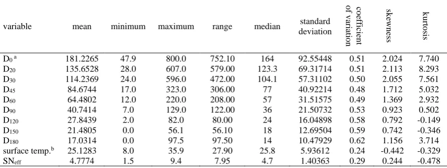
This section gives the results of the analysis obtained from three methods introduced in the previous section. Before embarking on a discussion of results, it is necessary to note that the modeling inputs were surface deflections and surface temperature of pavement, and the modeling target was SNeff. Table 3 presents the statistical characteristics of the dataset used in the study include mean, minimum, maximum, range, median, etc.

Table 3 Statistical characteristics of the study dataset

variable mean minimum maximum range median standard

deviation co efficie n t o f v ariati o n sk ewn ess k u rt o sis

D0 a 181.2265 47.9 800.0 752.10 164 92.55448 0.51 2.024 7.740

D20 135.6528 28.0 607.0 579.00 123.3 69.31714 0.51 2.113 8.293

D30 114.2369 24.0 596.0 472.00 104.1 57.31102 0.50 2.055 7.561

D45 84.6744 17.0 323.0 306.00 77 40.92214 0.48 1.712 5.032

D60 64.4802 12.0 220.0 208.00 57 31.51575 0.49 1.369 2.932

D90 40.7414 7.0 129.0 122.00 36 21.50732 0.53 0.923 0.502

D120 27.8439 2.0 82.0 80.00 24 16.04898 0.58 0.792 -0.149

D150 21.4805 0.0 56.1 56.10 18 12.69504 0.59 0.742 -0.346

D180 17.0314 0.0 97.5 97.50 14 10.47929 0.62 1.156 3.714

surface temp.b _25.1283 _8.0 _35.9 _27.90 _25.8 _5.93612 _0.24 _-0.442 _-0.329

SNeff 4.7774 1.5 9.4 7.95 4.7 1.40363 0.29 0.244 -0.478

a_D

i = Deflection at radius of i cm from loading center in FWD test b_{“Surface temp.” refers to temperature of asphalt surface}

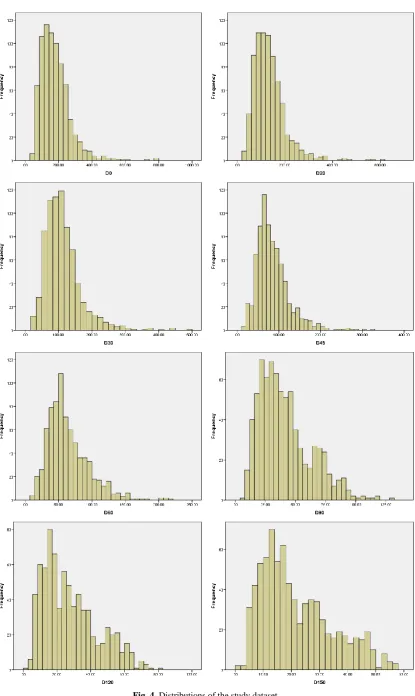
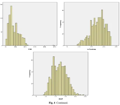
Table 3 gives basic information about the statistical state of the data. One of the most important statistical analyses is the correlation test. For determining the correlation of all variables with the target variable, the normality of the data must be determined. There are three methods to determine whether a variable is normal:

1. Skewness and kurtosis value (see Table 3) 2. Diagram of distribution (see Fig. 4)

(13)

13

(14)

14 Fig. 4 Continued.

First, the normality of SNeff is checked. The Skewness and kurtosis values are between -2 and +2. The diagram of distribution is almost similar to the normal diagram. Table 4 depicts the results of Kolmogorov-Smirnov and Shapiro-Wilk tests for SNeff. The significance level (Sig.) for both tests is less than 0.05 then, SNeff is not normal.

Table 4 Tests of normality for SNeff

Kolmogorov-Smirnov Shapiro-Wilk Statistic df Sig. Statistic df Sig.

.057 759 .000 .988 759 .000

Since SNeff is not normal, the Spearman correlation test should be used. Spearman’s correlation coefficients between input variables and SNeff presented in Table 5.

Table 5 Spearman’s correlation coefficient between input variables and SNeff

Variable D0 D20 D30 D45 D60 D90 D120 D150 D180 surface temp. Spearman’s

correlation coefficient

-0.7 -0.617 -0.533 -0.347 -0.176 0.038 0.137 0.169 0.223 -0.438

(15)

15

Table 6 Target and seven input categories selected for prediction

category no. inputs Target

1 D0, D20, D30, D45, D60, D90, D120, D150, D180, and Surface temp.

SNeff 2 AUPP, SCI, BDI, F2, F3, and Surface temp.

3 AUPP, SCI, BDI, Surface temp., and D0

4 AUPP, SCI, D0×Surface temp., D0 – D60, and D20 – D30 5 AUPP, SCI, BDI, D0×Surface temp., F2, and F3

6 D0 – D60, D0 – D45, D20 – D30, and

Surface temp. AUPP 7 AUPP, D0 – D45,

Surface temp.

(D0 – D60)×(D20 – D30), and

1

BDI×SCI×AUPP×(D0 – D60)×(D20 – D30)

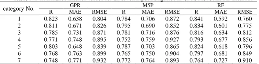
Modeling was performed using three methods GPR, M5P, and RF for each of the seven input categories. A comparison of modeling results and selection of the most suitable model was conducted using three criteria R, MAE, and RMSE. The values of R, MAE, and RMSE presented in Table 7.

Table 7 Performance metrics values for all seven input categories in GPR, M5P, and RF methods

category No. GPR M5P RF

R MAE RMSE R MAE RMSE R MAE RMSE

1 0.823 0.638 0.804 0.784 0.706 0.872 0.841 0.592 0.760 2 0.811 0.671 0.826 0.795 0.690 0.852 0.834 0.601 0.775 3 0.785 0.731 0.871 0.781 0.716 0.876 0.816 0.634 0.812 4 0.771 0.748 0.895 0.752 0.759 0.927 0.793 0.677 0.856 5 0.803 0.648 0.839 0.787 0.703 0.865 0.824 0.618 0.796 6 0.768 0.763 0.899 0.765 0.750 0.904 0.797 0.681 0.849 7 0.748 0.771 0.932 0.772 0.764 0.893 0.764 0.727 0.910

(16)

16

Fig. 5 Observed and predicted values of SNeff for GPR-1, M5P-2, and RF-1 models.

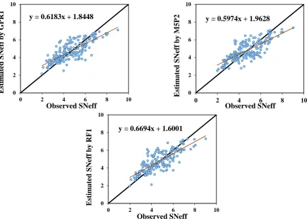
As Fig. 5, the purpose of Fig. 6 is to compare the observed SNeff and estimated SNeff values. In this figure, the observed SNeff plotted against the estimated SNeff for all three methods GPR1, M5P2, and RF1. Fig. 6 allows us to compare all three models numerically and more precisely. In Fig. 6, the most suitable model is the one that has a fit line equation of y = x. In this condition, the line slope is equal to one, and the line intercept is equal to zero. By examining Fig. 6, it is found that RF1 model is better than GPR1 and M5P2 models.

Fig. 6 Scatter plots of observed and predicted SNeff values for GPR-1, M5P-2, and RF-1 models. 1

3 5 7 9

0 30 60 90 120 150 180

SN

ef

f

Number of test data

Observed GPR1 M5P2 RF1

y = 0.6183x + 1.8448

0 2 4 6 8 10

E st im at ed S N ef f b y GPR 1 Observed SNeff

y = 0.5974x + 1.9628

0 2 4 6 8 10

E st im at ed S N ef f b y M5P 2 Observed SNeff

y = 0.6694x + 1.6001

0 2 4 6 8 10

(17)

17

Fig. 7 presents the Taylor diagram. Karl E. Taylor developed this diagram to aid the comparative evaluation of various models in a system. In this diagram, it is possible to reveal the degree of agreement between observed SNeff and estimated SNeff by GPR1, M5P2, and RF1 models. The mechanism of this diagram is based on three contours [65]:

❖ Blue contours

These contours represent the Pearson correlation coefficient.

❖ Orange contours

These contours describe RMSE error.

❖ Black contours

These contours exhibit the standard deviation.

In a Taylor diagram, each model is showed by a small colored circle. The model closer to the observation circle has better quality and higher prediction accuracy. Fig. 7 also confirms the superiority of RF1 model over GPR1 and M5P2 models.

Fig. 7 Taylor diagrams of predicted SN values.

By reviewing Figs. 5, 6 and 7, it can be concluded that the best modeling performed in this study is RF1.

5 Summary and conclusions

(18)

18

The main conclusions that could be drawn from this study are:

1. All three methods (GPR, M5P, and RF) had relatively the same accuracy in the prediction of SNeff, but RF yielded better results.

2. The thickness of the pavement layers was not required in the proposed methods, which obviated the need to perform the GPR test.

3. Replacing back-calculation methods with ML methods improved the reliability level and precision of the prediction process.

4. The main innovation of this paper was using surface temperature of pavement as an input variable which yielded acceptable results.

For future research, the authors suggest the following:

1. If equipment such as RWD and TSD approved by DOTs for PMS implementation, future modeling is suggested to do with the help of these types of equipment. These equipment eliminate traffic interference during pavement deflection recording, thus reduce costs and increase safety.

2. If researchers have access to traffic data, it is recommended that they apply this information in their modeling. This information is usually recorded by automated traffic counters and does not induce any problems for traffic flow and users.

3. In this study, the pavement sections selected from areas with various climatic conditions. Due to the limited number of data, the authors used all the data in modeling. For future research, if adequate data is available from different regions, it is recommended that to differentiate between diverse climatic conditions. For instance, three modelings performed for three distinct climates including warm, temperate, and cold areas. This method makes the models more applicable and will not need to be calibrated for use elsewhere.

6 References

1. Uddin Ahmed Zihan, Z., et al., Development of a structural capacity prediction model based on traffic speed deflectometer measurements. Transportation research record, 2018. 2672(40): p. 315-325.

2. Onyango, M., et al., Analysis of cost effective pavement treatment and budget optimization for arterial roads in the city of Chattanooga. Frontiers of Structural and Civil Engineering, 2018. 12(3): p. 291-299.

3. Kuo, C.-M. and T.-Y. Tsai, Significance of subgrade damping on structural evaluation of pavements. Road Materials and Pavement Design, 2014. 15(2): p. 455-464.

4. Lytton, R.L. Concepts of pavement performance prediction and modeling. in Proc., 2nd North American Conference on Managing Pavements. 1987.

5. Kargah-Ostadi, N., Y. Zhou, and T. Rahman, Developing Performance Prediction Models for Pavement Management Systems in Local Governments in Absence of Age Data. Transportation Research Record, 2019: p. 0361198119833680.

6. Elbagalati, O., et al., Development of the pavement structural health index based on falling weight deflectometer testing. International Journal of Pavement Engineering, 2018. 19(1): p. 1-8.

7. Abd El-Raof, H.S., et al., Simplified Closed-Form Procedure for Network-Level Determination of Pavement Layer Moduli from Falling Weight Deflectometer Data. Journal of Transportation Engineering, Part B: Pavements, 2018. 144(4): p. 04018052.

8. Nejad, F.M., et al., An image processing approach to asphalt concrete feature extraction. Journal of Industrial and Intelligent Information Vol, 2015. 3(1).

(19)

19

10. Karballaeezadeh, N., et al., Prediction of remaining service life of pavement using an optimized support vector machine (case study of Semnan–Firuzkuh road). Engineering Applications of Computational Fluid Mechanics, 2019. 13(1): p. 188-198.

11. Pinkofsky, L. and D. Jansen, Structural pavement assessment in Germany. Frontiers of Structural and Civil Engineering, 2018. 12(2): p. 183-191.

12. Liu, P., et al., Application of semi-analytical finite element method to analyze the bearing capacity of asphalt pavements under moving loads. Frontiers of Structural and Civil Engineering, 2018. 12(2): p. 215-221.

13. Dai, S. and Q. Yan. Pavement Evaluation Using Ground Penetrating Radar. in Geo-Shanghai 2014. 2014.

14. AASHTO, G., Guide for design of pavement structures. American Association of State Highway and Transportation Officials, Washington, DC, 1993.

15. Chen, R., et al., Prediction of shield tunneling-induced ground settlement using machine learning techniques. Frontiers of Structural and Civil Engineering, 2019: p. 1-16.

16. Abed, A., N. Thom, and L. Neves, Probabilistic prediction of asphalt pavement performance. Road Materials and Pavement Design, 2019: p. 1-18.

17. Abaza, K.A., Deterministic performance prediction model for rehabilitation and management of flexible pavement. International Journal of Pavement Engineering, 2004. 5(2): p. 111-121. 18. Dalla Valle, P., Reliability in pavement design. 2015, University of Nottingham.

19. Huang, Y.H., Pavement analysis and design. 1993.

20. Kargah-Ostadi, N., S.M. Stoffels, and N. Tabatabaee, Network-level pavement roughness prediction model for rehabilitation recommendations. Transportation Research Record, 2010. 2155(1): p. 124-133.

21. Yang, J., et al., Forecasting overall pavement condition with neural networks: application on Florida highway network. Transportation research record, 2003. 1853(1): p. 3-12.

22. Kargah-Ostadi, N. and S.M. Stoffels, Framework for development and comprehensive comparison of empirical pavement performance models. Journal of Transportation Engineering, 2015. 141(8): p. 04015012.

23. Noureldin, A.S., New scenario for backcalculation of layer moduli of flexible pavements. Transportation Research Record, 1993(1384).

24. Jameson, G., Development of procedures to predict structural number and subgrade strength from falling weight deflectometer deflections. ARRB Transport Research, 1993.

25. Rohde, G.T., Determining pavement structural number from FWD testing. Transportation Research Record, 1994(1448).

26. Rohde, G.T., et al. The calibration and use of HDM-IV performance models in a pavement management system. in Fourth International Conference on Managing Pavements. Durban, South Africa. 1998.

27. Schnoor, H. and E. Horak. Possible method of determining structural number for flexible pavements with the falling weight deflectometer. in Abstracts of the 31st Southern African Transport Conference (SATC 2012). 2012.

28. 336, C., Information Gathering Report, in Falling weight deflectometer. 1998.

29. Crook, A.L., S.R. Montgomery, and W.S. Guthrie, Use of falling weight deflectometer data for network-level flexible pavement management. Transportation Research Record, 2012. 2304(1): p. 75-85.

30. Dasari, K.V., Deflection based condition assessment for Rolling Wheel Deflectometer at network level. 2013.

31. Hoffman, M.S., Direct method for evaluating structural needs of flexible pavements with Falling-Weight Deflectometer deflections. Transportation Research Record, 2003. 1860(1): p. 41-47.

32. Abdel-Khalek, A., et al., A model to assess pavement structural conditions at the network level. Transportation Research Record, 2012.

(20)

20

34. Abd El-Raof, H.S., et al., Structural number prediction for flexible pavements based on falling weight deflectometer data. 2018.

35. Gedafa, D.S., et al., Network-level flexible pavement structural evaluation. International Journal of Pavement Engineering, 2014. 15(4): p. 309-322.

36. Elbagalati, O., et al., Prediction of in-service pavement structural capacity based on traffic-speed deflection measurements. Journal of Transportation Engineering, 2016. 142(11): p. 04016058.

37. Kavussi, A., et al., A new method to determine maintenance and repair activities at network-level pavement management using falling weight deflectometer. Journal of Civil Engineering and Management, 2017. 23(3): p. 338-346.

38. Salvi, R., et al., Use of Ground-Penetrating Radar (GPR) as an Effective Tool in Assessing Pavements—A Review, in Geotechnics for Transportation Infrastructure. 2019, Springer. p. 85-95.

39. Benedetto, A., et al., An overview of ground-penetrating radar signal processing techniques for road inspections. Signal processing, 2017. 132: p. 201-209.

40. Horak, E., et al., Revision of the South African pavement design method. 2009, Draft Contract Report, No. SANRAL/SAPDM/B-2/2009-01.

41. Ministry of Roads and Urban Development, T.S.M.L.c.; Available from: https://www.tsml.ir. 42. Guo, H., X. Zhuang, and T. Rabczuk, A Deep Collocation Method for the Bending Analysis of

Kirchhoff Plate. CMC-COMPUTERS MATERIALS & CONTINUA, 2019. 59(2): p. 433-456.

43. Anitescu, C., et al., Artificial neural network methods for the solution of second order boundary value problems. Computers, Materials & Continua, 2019. 59(1): p. 345-359.

44. Hamdia, K.M., et al., Computational Machine Learning Representation for the Flexoelectricity Effect in Truncated Pyramid Structures. Computers, Materials & Continua 59 (2019), Nr. 1, 2019.

45. Hamdia, K.M., et al., A novel deep learning based method for the computational material design of flexoelectric nanostructures with topology optimization. Finite Elements in Analysis and Design, 2019. 165: p. 21-30.

46. Sun, A.Y., D. Wang, and X. Xu, Monthly streamflow forecasting using Gaussian process regression. Journal of Hydrology, 2014. 511: p. 72-81.

47. Williams, C.K. and C.E. Rasmussen, Gaussian processes for machine learning. Vol. 2. 2006: MIT press Cambridge, MA.

48. Arthur, C.K., V.A. Temeng, and Y.Y. Ziggah, Novel approach to predicting blast-induced ground vibration using Gaussian process regression. Engineering with Computers, 2019: p. 1-14.

49. Li, J.J., et al., Estimating urban ultrafine particle distributions with gaussian process models. Research@ Locate14, 2014: p. 145-153.

50. Chu, W. and Z. Ghahramani, Gaussian processes for ordinal regression. Journal of machine learning research, 2005. 6(Jul): p. 1019-1041.

51. Samui, P., Utilization of Gaussian process regression for determination of soil electrical resistivity. Geotechnical and Geological Engineering, 2014. 32(1): p. 191-195.

52. Samui, P. and J. Jagan, Determination of effective stress parameter of unsaturated soils: A Gaussian process regression approach. Frontiers of Structural and Civil Engineering, 2013. 7(2): p. 133-136.

53. Quinlan, J.R. Learning with continuous classes. in 5th Australian joint conference on artificial intelligence. 1992. World Scientific.

54. Wang, Y. and I.H. Witten, Induction of model trees for predicting continuous classes. 1996. 55. Singh, T., M. Pal, and V. Arora, Modeling oblique load carrying capacity of batter pile

groups using neural network, random forest regression and M5 model tree. Frontiers of Structural and Civil Engineering, 2019. 13(3): p. 674-685.

(21)

21

57. IH, W. and E.D. Mining, Practical machine learning tools and techniques. United State: Morgan Kauffman, 2011.

58. Blaifi, S.-a., et al., M5P model tree based fast fuzzy maximum power point tracker. Solar Energy, 2018. 163: p. 405-424.

59. Breiman, L., et al., Classification and regression trees. Wadsworth Int. Group, 1984. 37(15): p. 237-251.

60. Breiman, L., Random forests. Machine learning, 2001. 45(1): p. 5-32.

61. Loh, W.Y., Classification and regression trees. Wiley Interdisciplinary Reviews: Data Mining and Knowledge Discovery, 2011. 1(1): p. 14-23.

62. Sadler, J., et al., Modeling urban coastal flood severity from crowd-sourced flood reports using Poisson regression and Random Forest. Journal of hydrology, 2018. 559: p. 43-55. 63. Sun, H., et al., Assessing the potential of random forest method for estimating solar radiation

using air pollution index. Energy Conversion and Management, 2016. 119: p. 121-129. 64. Xu, T., et al., Quantifying model structural error: Efficient Bayesian calibration of a regional

groundwater flow model using surrogates and a data‐driven error model. Water Resources Research, 2017. 53(5): p. 4084-4105.

65. Taylor, K.E., Summarizing multiple aspects of model performance in a single diagram. Journal of Geophysical Research: Atmospheres, 2001. 106(D7): p. 7183-7192.

Appendix

Abbreviation Meaning

PMS Pavement Management System

DT Destructive Testing

NDT Non-Destructive Testing

FWD Falling Weight Deflectometer

SN Structural Number

RSL Remaining Service Life

DOL Overlay Thickness

GPR Ground Penetrating Radar

SNeff Effective Structural Number

ML Machine Learning