Analyzing Software Artifacts through Singular Value Decomposition to Guide Development Decisions

(1)

ABSTRACT

SHERRIFF, MARK STEPHEN. Analyzing Software Artifacts through Singular Value Decomposition to Guide Development Decisions. (Under the direction of Laurie A. Williams.)

During development, programming teams will produce numerous types of software development artifacts. A software development artifact is an intermediate or final product that is the result or by-product of software development. Hidden relationships and structures within a software system can be illuminated through singular value decomposition using software development artifacts, and these relationships can be leveraged to help guide software development questions regarding the interactions among software files.

The goal of this research is to build and investigate a framework called Software Development Artifact Analysis (SDAA) that uses software development artifacts to illuminate underlying relationships within a system. SDAA provides guidelines for selecting and gathering software development artifacts, discovering relationships, and then leveraging the insights gained through the analysis of those relationships. We use singular value decomposition (SVD) to generate the relationships from a matrix of software development artifact metrics.

(2)

(3)

Analyzing Software Artifacts Through Singular Value Decomposition to Guide Development Decisions

by

Mark Stephen Sherriff

A dissertation submitted to the Graduate Faculty of North Carolina State University

in partial fulfillment of the requirements for the Degree of

Doctor of Philosophy

Computer Science

Raleigh, North Carolina 2007

APPROVED BY:

_________________________ _________________________ Dr. Thomas L. Honeycutt Dr. Jason A. Osborne

(4)

DEDICATION

(5)

BIOGRAPHY

Mark S. Sherriff was born November 9, 1979 in Salisbury, North Carolina. Mark

grew up in Salisbury and Rock Hill, SC, and received his first computer (a 486 SX 25 Mhz)

in the eighth grade. Since then, he’s been fascinated by technology, computing, and how to

make the experience better for everyone, from developers to end-users. Mark received his

B.S. from Wake Forest University in Computer Science in 2002. In 2004, Mark earned his

M.S. from North Carolina State University on the way to his Ph.D. in 2007.

As a technology enthusiast, Mark enjoys everything from building computers to web

design to playing video games. He also enjoys cooking, traveling, and has been involved in

(6)

ACKNOWLEDGEMENTS

As any doctoral student will attest, the pursuit of a PhD cannot be done alone and

most certainly can only come about with the help and support of many people. Over the past

five years, Dr. Laurie Williams has been a continual source of wisdom, support, and

encouragement for me. In a field that is constantly searching for women in every possible

role from student to professor, I have had the fortune of working with one of the best. Words

cannot adequately express the gratitude that I have for her seemingly unending source of

patience, words of encouragement, and insights into software engineering. When I came to

NC State, it is fair to say that I was a good student, but really had no inkling as to what my

future chosen profession actually entailed. Laurie has been an exceptional mentor, a good

friend, and the main academic reason that I am even writing this paragraph. I sincerely hope

that she has gained as much from our time together as I have, and hopefully it is something

other than my tendency to exaggerate greatly.

During my time at NC State, I also had the opportunity of working with a man who

once told me that he appeared in numerous PhD acknowledgement sections as a person who

gave a key insight. It didn’t take me long to discover just why that was the case. Dr. J.

Michael Lake gave me not only a key insight into this research; he also helped provide the

means and amazing amounts of guidance. It is almost a certainty that without his assistance,

this dissertation would be about something else completely and would have a date perhaps a

year or two later. Mike’s ability to dissect a problem and his tenacity at solving it served as

an example to me during my time at IBM. To him, Jim Fletcher (my manager at IBM), and

(7)

University has been extremely important in the lives of numerous doctoral students. The

atmosphere of support at IBM for students and research is refreshing and much appreciated.

In addition to the research support from IBM, several other individuals and

organizations were generous in their research and financial support. The Center for

Advanced Computing and Communication has been a continual source of financial support

for my research and for others in my research group. Specifically, the support and

encouragement of Brad Martin through the National Science Foundation has been of

immense benefit to me over my five years at NCSU.

I would also like to thank my doctoral committee. My first real impression of Dr.

Mladen Vouk was during my Master’s examination, where he, while eating pastries I had

made the night before, asked question after question, causing me to doubt nearly everything I

showed. Afterwards, thankfully after passing me on the exam, he simply said to me “the

lesson is to not put anything extra on your slides, because that is where the questions arise.”

As I mentioned earlier, I have a tendency to exaggerate, and this simple statement changed

the way I looked at how I would present research from then on. I am pleased that I got to

know him better during our time working for ISSRE, and I am sincerely glad he agreed to be

on my committee. I got to know Dr. Tom Honeycutt through his software engineering

course, where, I can safely say, he portrayed the field in ways I had never considered.

Always a man with a smile and a pipe, I am thankful for his insights into my work and his

interest into my progress over these five years. Dr. Jason Osborne was introduced to me

through the research of one of my colleagues. Ever since then, his guidance in statistical

(8)

Speaking of our research group, I often heard second hand around the department

about “Laurie’s students” and what we were up to. I am extremely proud to say that I am a

member of the Realsearch Group along with some of the best people I have met at NC State.

The thing that makes me most proud about our group is that, unlike a lot of graduate

students, we are involved in our department. From open houses, to conferences, to managing

labs, to being teaching assistants – it makes me proud to know that I work with people who

are not only good researchers, but also excel at teaching and service, which is important for

any academic. If I went into the specific reasons why I respect each of these people, I dare

say it may be longer than the dissertation itself. Thanks to Nachi Nagappan, the first student

mentor I had. Thanks to Lucas Layman and Sarah Smith Heckman, the other two corners of

what I thought of as “the trio” with me, as we collectively served as Laurie’s right hand in

teaching and whatever else that needed to be done. Thanks to Dright Ho, Jiang Zheng,

Yonghee Shin, Michael Gegick, Hema Srikanth, Andy Meneely, Mei Nagappan, Stephen

Thomas, Paul Otto, Laurie Jones, and Colin Butler. My sincere thanks to the staff at NC

State for all that they do for the department; without them, we students most certainly would

not graduate.

The love and support of family needed to complete this journey can never be

exaggerated. Thanks to my father, Steve, who taught me my first lessons about technology

and research. Thanks to my mother, Nancy, whose support is never-ending, even when her

knowledge of technology didn’t allow her to follow along any more. Thanks to my siblings,

Beth and Kevin, who balance my geekness quite effectively in the family. Thanks to my

in-laws, Dan and Linda Jones, who accepted me into their family without the slightest

(9)

Saved for last is of course my wife, Amanda, without whom I would be lost. She is

by far the smartest woman I know, who could have gone into any field she set her mind to,

and she chose to teach young children about reading. The sacrifices I see her make day after

day for her kids are astonishing and come with an amazing amount of love. She is my

(10)

LIST OF FIGURES

Figure 3.1 SDAA steps ……….. 13

Figure 4.1 Graphs of top 250 singular values for the three minor releases ……... 43

Figure 4.2 Charts of comparisons of impact sets ……….. 47

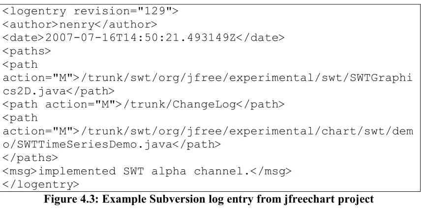
Figure 4.3 Example Subversion log entry from jfreechart project ……… 52

Figure 4.4 Comparison of ordering of true and false positives ………. 63

Figure 5.1 Percentage of tests recommended to be rerun ………. 76

Figure 5.2 Percentage matches in future data by regression test priority ………. 77

Figure 5.3 Change in non-source file example ……….. 79

Figure 6.1 ASA alert signature cluster singular values ……… 99

Figure 6.2 ASA alert signature cluster singular values ……… 108

Figure 6.3 Results of using regression analysis to predict failure density (Run 1) . 119

(12)

LIST OF TABLES

Table 3.1 Types of software development artifacts ………. 14

Table 4.1 Sample change record information ……….. 35

Table 4.2 Results from association cluster creation ………. 44

Table 4.3 Investigation results ……….………. 49

Table 4.4 Selected open source projects ……….. 52

Table 4.5 Impact method size summary ……….. 54

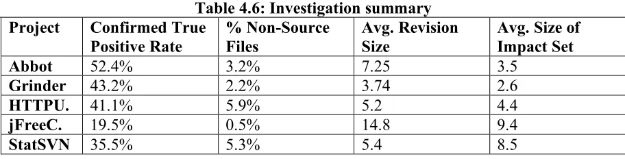
Table 4.6 Investigation summary ……….……… 54

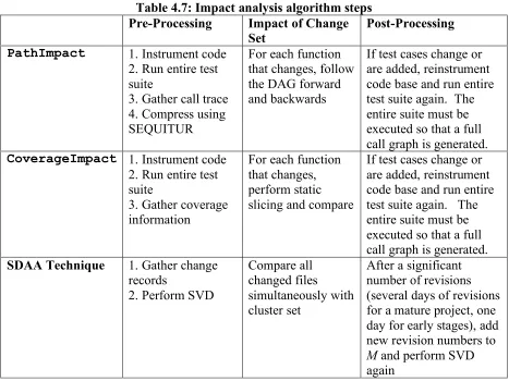
Table 4.7 Impact analysis algorithm steps ………... 60

Table 4.8 Time and resource concerns for impact analysis algorithms ………... 60

Table 5.1 Model recommendations ……….……… 76

Table 6.1 Summary of effects of applying ASA alert signatures ……… 104

Table 6.2 Build dates ……….……….. 106

Table 6.3 Case study overview ……….……… 107

Table 6.4 Results summary ……….………. 113

Table 6.5 Summary of spearman rank correlation for 1545 files ……… 115

Table 6.6 Further analysis of spearman rank correlation for 1545 files ……….. 118

Table 6.7 Summary of case studies ……….……… 122

Table 7.1 Impact analysis case study overview ………... 126

Table 7.2 Regression test prioritization case study overview ……….. 127

(13)

CHAPTER 1

INTRODUCTION

Software development managers balance lifecycle costs during development and maintenance with potential profits from sales [21]. Releasing a software system early may gain an initial boost in profits by being first to market, but profit and customer confidence could easily disappear if field failures are found due to a lack of quality. Thus, researchers in the field of software reliability engineering have developed numerous techniques that can direct developers to areas of the code base that contain faults1 [22, 23, 28-33, 35-37, 43-45, 47-50]. However, many of these techniques require computationally and resource intensive aspects, such as large call graphs, that can take hours to run and several gigabytes of disk space [9]. Based upon how the system is being used in the field and the relative severity of some of these potential faults, delaying product release to address these potential faults may allow competitors to enter the market earlier and gain a larger market share, thus eliminating some of the cost-benefit of performing some of the reliability techniques. Software development managers could benefit from information that can be provided quickly and efficiently during the development process to provide guidance in determining when software is “good enough” to release.

(14)

Some insight into when to release a product may be gathered from the information generated during the development process itself. During development, programming teams will produce a variety of software development artifacts. A software development artifact is an intermediate or final product that is the result or by-product of software development [24, 25]. Some software development artifacts are created by the development team, such as source code and design documents. However, other development artifacts, such as change records in a source control system, defect records, and test case logs, are generated throughout the process and are used for support purposes [1].

For example, change records might be referenced to track development progress or to learn the current version of a file in the system. However, these development artifacts can also provide information about underlying relationships within a system that would normally not be apparent [4, 6, 14, 27, 52-55, 61, 63]. Change records can show how components interact with one another or how a system is evolving during development by examining what areas of the system change together and where new tracks are appearing [4, 6]. A track

is a grouping of files that have been changed together to address a defect. Managers can use detailed change information to monitor progress throughout development as sections of code enter and exit test. Testers could use information about how components of a system tend to change together as well, since they could use this knowledge to direct their testing efforts whenever a new track is created.

(15)

There are three main advantages of using historical, empirical data as opposed to semantic data when directing development efforts. First, the cost in system resources can be exceedingly high using a semantic technique. Research by Breech et al. in comparing dynamic impact analysis techniques showed that from a selection of eight programs, seven programs required either more disk space than the test machine had free (15GB) or took over two hours to run [9]. The second advantage is that historical data can show where previous maintenance has taken place or how the system is being used in the field. With this actual operational profile information, development and maintenance efforts can be prioritized to address areas of the system that are under more use. Finally, using software development artifacts allows analysis techniques to treat all files in a system the same, whether those files are source code, media files, documentation, or any other file type. Dynamic fault analyses may only be limited to source code of one particular language; however, faults that appear because of non-executable files can be just as problematic in a software system [20, 55].

(16)

often being tested together. These association clusters could correspond to functional requirements or execution paths, thus exhibiting underlying relationships of the software system that might not readily be apparent. Earlier research has shown that software development artifacts can be used in software change analysis to discover underlying relationships within a code base [4, 6, 14, 27, 52-55, 61, 63]. These relationships have in previous research been used to represent design decisions and for program comprehension. Our work adds to this body of knowledge by introducing a new technique for illuminating these relationships and then leveraging them to help guide development and maintenance decisions.

In empirical software engineering, theory should be integrated into research to advance the body of knowledge [15]. Through this research, an explanation type theory will be built and evaluated. An explanation type theory, also called a “theory for understanding,” is used to provide understanding of a phenomenon, however its goal is not to predict precise results. The main purpose of theories of this type is to guide others as to how the world may be viewed under certain circumstances [15].

The explanation type theory being built and evaluated through this research is stated as follows:

Decision support for software development decisions is more resource efficient with respect to time, memory, and developer overhead when based upon relationships between software artifacts illuminated via a singular value decomposition of actual usage information

(17)

The core motivation behind our theory and this research is providing decision support for industry in instances where resource efficiency and overall time are critical, such as when a product needs to be released in the confines of a strict schedule. As has been discussed, there are numerous techniques available that can, with enough time and computational resources, can provide effective and safe impact analysis and regression test selection. However, there are also instances in industry when time and resource constraints limit the amount of effort that can be put forth into these techniques. We want to address this issue by adding to the body of software engineering knowledge regarding techniques that can provide effective decision support with less overall resources for non-critical software systems, thus helping teams to make software quality decisions that ordinarily could not. There is a trade off of inclusiveness and precision with the resources required to execute the technique, and we are exploring the latter option in this work.

The main contribution of this research is a process that helps guide developers through the use of singular value decomposition (SVD) and software development artifacts to provide insight into various software development decisions. The decision areas include impact analysis, regression test prioritization, and the filtering of static analysis results.

(18)

compiled into a matrix that relates a particular code unit to other code units with regards to that artifact. For example, if a small system consisted of five files, the matrix would be 5x5 and the values in the matrix would correspond to metrics about a particular development artifact, such as the number of times two files have changed together. A singular value decomposition (SVD) [13] is performed on the matrix to generate the association clusters. The results of the SVD can then be utilized to guide software development decisions.

In this work, we will describe the steps of the SDAA framework and how they are used to help create analysis techniques based upon development artifacts and SVD. We will specifically discuss three techniques that we created using SDAA, including impact analysis, regression test prioritization, and static analysis filtering. To validate our techniques, we performed industrial case studies with each with the cooperation of IBM. Further, we also evaluated our techniques with six different open source projects to test how they would work outside of an industrial setting. The background and related work for each technique will be provided in the corresponding chapter.

(19)

(20)

CHAPTER 2

BACKGROUND

In this chapter, we will discuss the general background to the SDAA framework. In particular, we will examine the use of singular value decomposition in software engineering research and other uses of software development artifacts.

2.1 SINGULAR VALUE DECOMPOSITION

Singular value decomposition (SVD) is a linear algebra technique that decomposes a given matrix into three component matrices [13]: (1) the left singular vectors; (2) a set of singular values; and (3) and right singular vectors. The two matrices that are made up of singular vectors provide information about the structure of the original matrix. The singular values describe the strength of the given components of the original matrix. The SVD theorem [13] states that given a matrix M, then there exists a decomposition of M such that

T

USV M = .

(21)

coordinates that generated a three-dimensional shape, then that shape could be constructed from the rotational information in U and V, along with stretching the shape out to its proper size with the information in S [60]. This type of decomposition can be important and useful in that the rotational matrices isolate the key components of the original matrix, finding relationships between the various data points, while the strength matrix indicates which of the key components illuminated in the rotational matrices are the most important [13, 60]. In our research, this core idea of isolating key components of the original matrix is the basis for using the SVD. When the matrix is comprised of change records, fault information, or some other data from the development process, these key components highlight underlying structures in the code base.

The SVD has other uses in computing. For instance, this technique can be used in image and signal compression. A gray scale image could be represented as a two-dimensional matrix made up of intensity values, indicating the darkness of a particular pixel. In this instance, we could treat the image matrix itself as the original M matrix and perform a SVD on it. Once the decomposition is completed, the resulting matrices, USVT_{, can also be} represented as the sum of component matrices, as shown in Equation 2.1:

T k k k k T

T _u _s _v _u _s _v

v s u

M = ₁ ₁_,₁ ₁ + ₂ ₂_,₂ ₂ +...+ _, (2.1)

(22)

Osinski et al. created a clustering algorithm based upon SVD to improve search queries on a set of documents [38]. They built an original matrix based upon keywords in the document set. The SVD was performed on this matrix to generate clusters of documents that were similar based on their keywords. Enough clusters were gathered to account for 90% of the variability of the original matrix, with the remaining clusters discarded as signal noise [38]. The documents were then assigned to clusters based upon which cluster they had the closest association with. Anecdotal evidence from users who were presented with the clusters generated with this study found that 70-80% of the clusters were useful and over 75% of identified cluster labels were correct [38].

2.2 USING SOFTWARE DEVELOPMENT ARTIFACTS

(23)

(24)

CHAPTER 3

SOFTWARE DEVELOPMENT ARTIFACT

ANALYSIS (SDAA)

SDAA is a framework that provides developers the means to step through the application of SVD analysis with software development artifacts to help guide development decisions. The specific development decisions can vary between projects and teams, depending on what artifacts are available and what the team is interested in examining. In this research, we highlight three specific techniques derived from SDAA to guide development decisions: impact analysis, regression test prioritization, and filtering static analysis alerts. The possible development decisions are not limited to these three, and we will describe others in Section 3.1.

(25)

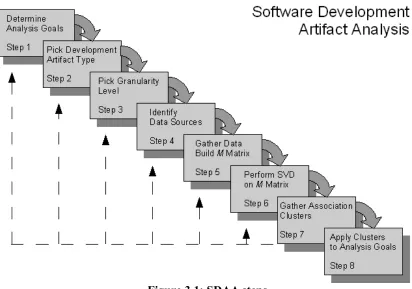
clusters, and interpreting the results of the analysis. Figure 3.1 outlines the steps of the SDAA. Each of these will be described in the subsequent subsections.

Figure 3.1: SDAA steps

3.1 STEP 1: DETERMINE ANALYSIS GOALS

(26)

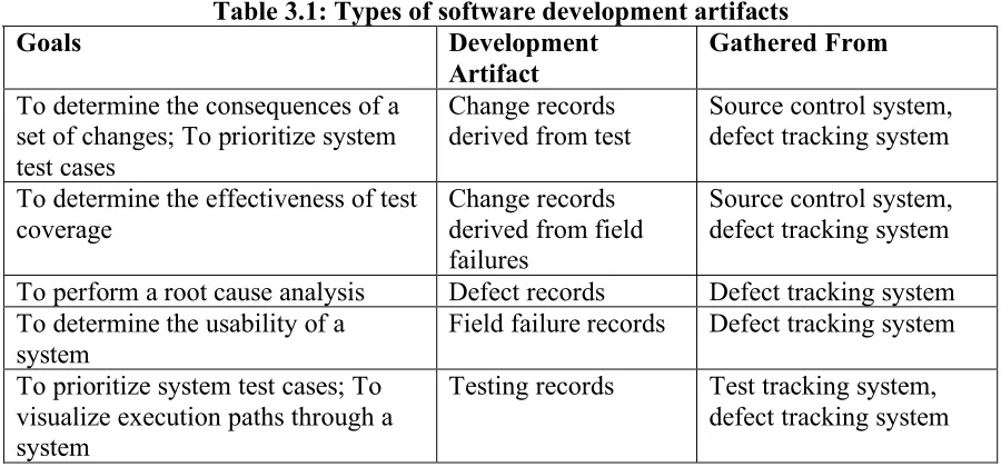
Table 3.1: Types of software development artifacts

Goals Development

Artifact

Gathered From

To determine the consequences of a set of changes; To prioritize system test cases

Change records

derived from test Source control system, defect tracking system To determine the effectiveness of test

coverage Change records derived from field failures

Source control system, defect tracking system To perform a root cause analysis Defect records Defect tracking system To determine the usability of a

system

Field failure records Defect tracking system To prioritize system test cases; To

visualize execution paths through a system

Testing records Test tracking system, defect tracking system

3.2 STEP 2: PICK DEVELOPMENT ARTIFACT TYPE

(27)

together. Information from defect tracking systems allows us to isolate changes to those made under specific circumstances. For example, changes derived from defects found during system test could be compared to changes derived from field failures discovered by customers.

Defect records found in defect tracking systems can also provide valuable information. Defect records could be gathered to find associations based on particular classes or types of defects, such as null pointer dereferences. If specific defect classification information is not present, then the natural language text of the defect descriptions could be used to make further associations. Field failures could also be examined in a similar fashion, providing information about what areas of the system users are having difficulties with. Musa created similar clusters of failure sets to aid in the description and tracking of software defects [29].

(28)

3.3 STEP 3: PICK GRANULARITY LEVEL

Once the type of artifact has been determined, the granularity level of the artifact will determine what type of code unit must be gathered for the analysis. We define the granularity level of an artifact to be the level of abstraction in the software system at which the analysis will be performed, such as line of code, method, class, file, or package. The granularity level should be appropriate for the analysis goal as each different type of code unit will portray a distinct view of the functional modular structure of the system. For instance, if directories or Java packages are selected as the code unit granularity, then the analysis will specifically target connections between these higher level components. If files are chosen as the code unit, then the analysis will still pick up some of the logical component interconnections, but will also provide information about which files are most important within its own component.

(29)

3.4 STEP 4: IDENTIFY DATA SOURCES

Source control systems are a valuable source for gathering development artifacts. When a developer checks a file in to a source control system, the system typically records the time of the check-in along with information about the developer and the nature of the change. Individual changes can be often be linked together into tracks, either through a specific mechanism in the source control system that records that information or by examining change record check-in information. A track is a grouping of files that have been changed together to address a defect. With information regarding tracks, we are able to ascertain how files, directories, packages, or other code units change together.

3.5 STEP 5: GATHER DATA AND BUILD

M

MATRIX

After the granularity and the artifacts for the analysis have been identified, an analysis matrix should be generated that contains the software development artifact code units along each axis. If the analysis is looking for relationships among a single type of artifacts, such as files that change together or static analysis alerts that tend to appear together, then the M

matrix will be a symmetric matrix, as shown in Equation 3.1.

!

M=

(30)

However, a non-symmetric matrix is perfectly acceptable if the analysis is looking for a relationship between two different development artifact types, such as what static analysis alert types appear in post-release field failures.

The values within the analysis matrix show how the code units interact through the development artifact and determine how the association clusters will be interpreted. For example, if the values in the matrix indicate the number of times that two files have changed together in response to a failure, then the association clusters will represent failure paths found in the system and files that are likely to be linked in some way. However, if the data set is limited to only field failures, then the analysis is focused more on user operational profiles and what areas of the system users are executing and discovering system failures. Further, if we are using two types of artifacts in a given analysis, we place the development artifact of most interest on the rows of M, which precipitates a need to use U for gathering association clusters because the row artifact designations will stay the same, while the columns become the association cluster identifiers. For example, if we want to see how static analysis alerts are related through files and what alert types tend to appear together in files, we would use alert types as the rows of M and files as the columns.

3.6 STEP 6: PERFORM SVD ON

M

MATRIX

(31)

! ! ! ! ! ! " # $ $ $ $ $ $ % & = 17 12 0 0 0 12 15 0 0 0 0 0 24 21 0 0 0 21 31 10 0 0 0 10 25 5 4 3 2 1 5 4 3 2 1 F F F F F M F F F F F (3.2) !

U=V =

".29 0 .9 .31 0

".76 0 ".02 ".56 0 ".59 0 ".43 .69 0 0 ".68 0 0 ".74

0 ".74 0 0 .68

# $ % % % % % % & ' ( ( ( ( ( ( (3.3) ! ! ! ! ! ! " # $ $ $ $ $ $ % & = 9 . 3 0 0 0 0 0 1 . 4 0 0 0 0 0 8 . 24 0 0 0 0 0 4 . 28 0 0 0 0 0 1 . 51

S (3.4)

The U and V matrices provide information as to the structure of the association clusters, while the singular values from the S matrix represent the amount of variability each association cluster contributes to the original analysis matrix. Note that U and V are equal, due to M being a symmetric matrix. The U and V matrices provide an orthonormal basis that we will use generate the association clusters.

Another way to view the SVD of M is by looking at USVT as a sum of sub-matrices [13, 60]. By taking the k sub-matrices out of n total sub-matrices (where n is the rank of M

(32)

T T T T T k i T i i i i T v s u v s u v s u v s u v s u M v s u M USV M 5 5 , 5 5 4 4 , 4 4 3 3 , 3 3 2 2 , 2 2 1 1 , 1 1 1 , + + + + = = =

!

= (3.5)

Each of these sub-matrices represents an association cluster. Notice that each association cluster sub-matrix is made up of one singular value from S and from identical vectors from U

and V.

3.7 STEP 7: GATHER ASSOCIATION CLUSTERS

Once the SVD has been performed on an M matrix, the association clusters can be gathered from the U matrix. If M is a symmetric matrix, then U and V are equivalent. If M is asymmetric, then U and V will contain different values. However, the clusters gathered from

U often are the same as those from V, but with different singular values. Thus, by examining

U, we will still get a good sense of the interconnections within the system.

In the U matrix, the development artifacts appear in the rows of the matrix, while the association clusters appear in the columns. Every artifact type that has a value in an association cluster column, however, does not necessarily become a part of that cluster. A threshold value is used to determine if the “strength” of the interconnection is high enough to warrant inclusion. During the course of this research, we will discuss our evaluation of threshold values.

(33)

provides the percentage of how representative the cluster is of the original matrix. A high singular value indicates that that association cluster is more prominent in the analysis matrix, due to a greater number of changes that have occurred. A high singular value could be indicative of a particularly problematic section of code or a new feature that has just been introduced into the system and is experiencing its first rigorous testing.

Duplicate clusters and clusters that are subsets of other clusters can often appear in this type of analysis. The third association cluster shown in Equation 3.3 is a subset of the first cluster, while the fourth association cluster is comprised the exact same files as the first cluster. All three sets of files contain different values associated with the files. The singular values of these clusters provide some indication as to how they should be analyzed. The first cluster has a singular value of 51.1, representing 45% of the overall variability in the matrix; the third cluster has a singular value of 24.8, representing 22%; and the fourth cluster has a singular value of 4.1, representing 4%. These percentages are found through dividing the singular value by the sum of all the singular values and show that the first cluster defines the majority of the information regarding these files. Clusters three and four are, in effect, the same as the first cluster.

(34)

3.8 STEP 8: APPLY CLUSTERS TO ANALYSIS GOALS

In this step, association clusters are now available that describe a type of relationship in the system between various system artifacts. How these relationships are interpreted and acted upon is dependent on the overall goal of the analysis and the type of artifacts used. Take, for example, a matrix M that is comprised of static analysis alert types as the rows and files as the columns, and the values of the matrix represent the number of times that a given alert type appears in a file. Then the resultant clusters from the analysis indicate what static analysis alert types appear together. Using this information, developers could begin to look for patterns in their development mistakes and could look for those patterns whenever static analysis tools are used.

3.9 LIMITATIONS

(35)

in the system, since there would at that point be no historical evidence as to how that module interacts with the rest of the system.

3.10 SUMMARY

In this chapter, we have outlined the steps in the SDAA framework for using software development artifacts and SVD to help guide development decisions. The eight steps are intended to be a guide as developers and managers seek to incorporate mathematically rigorous methodology for highlighting relationships between different aspects of a software system. Throughout the remainder of this work, we will describe our experiences using SDAA and the techniques born from it. Empirical results to date, as will be discussed, indicate the use of the technique is appropriate for non-critical software, particular products with time and resource constraints.

In our work, nearly all of these steps were automated using simple scripts and Java programs. These scripts gathered the development artifacts from a software development tool, such as a source control system or static analysis program, and put the artifacts into a MySQL database for easier management. We then used Matlab scripting to query the database, perform the SVD, and record the generated associated clusters. Matlab scripts were also used to apply the clusters by comparing the clusters to incoming sets of development artifacts. An example script is provided in Appendix A.

(36)

(37)

CHAPTER 4

IMPACT ANALYSIS USING DEVELOPMENT

ARTIFACTS

(38)

determining the effects of a change through actual execution paths. Current impact analysis techniques that utilize call graphs, dynamic executions of the system, or static code analysis mainly focus on changes in the system’s source code [10, 18, 37, 41].

End users of a system, however, can find numerous failures that do not originate in source code, but in non-compilable, non-executable files, such as media files, documentation files, and help files [56]. Failures that arise in these non-executable areas can be just as severe as a fault within the source code itself [20]. While some dynamic impact analysis techniques have been shown to be safe2 under most circumstances [36, 37], these techniques may not be capable of determining the impact of a change that occurs solely in a non-executable file that is never compiled with the source code. Some static impact analysis techniques can take into account these non-executable files, however these techniques do not consider trends in actual system usage or the fault-proneness of the set of files impacted. Without usage trends, the results of semantic impact analysis may require more effort to determine exactly which areas of the system have the highest risk of containing a latent fault [36].

Using SDAA, our goal is to provide an impact analysis methodology that uses historical change records for both executable and non-executable files in a software system

to identify potentially-affected areas of a system modification. By utilizing change records, we can show what files tend to change together for development purposes or in response to repairing faults in the system. A change record artifact provides the documentation for a change made to a single file for the purpose of a system modification. Analyzing how tracks

(39)

change can provide an indication as to how files interact with one another to perform a system modification [4, 6]. Our technique’s main difference from other impact analysis techniques is that ours is based on historical change data rather than execution and/or code semantics. The benefit we gain using historical change data is that every file stored in change management is analyzed similarly, whether that file contains source code, object code, media, or documentation. By leveraging change records as the software development artifact, SDAA provides an empirical method for determining the impact of a change, placing focus on the areas of the system that have been used in testing and by the customer.

In this chapter, we will describe how SDAA can be leveraged through change records to provide an impact analysis of a proposed change to a software system. We will describe in this chapter related impact analysis work and how these techniques correlate with our impact analysis methodology. We will also discuss an industrial case study and an open source case study on the effectiveness of our impact analysis technique and how our results compare to those of other impact analysis techniques in identifying potentially affected areas of a system. Further, we will discuss how this technique can apply to projects that may not follow rigorous development methodologies, such as open-source projects.

4.1 BACKGROUND

Dynamic impact analysis techniques rely upon information gathered from a system during runtime, often gathered through execution of the system or test suites with an instrumented code base [18, 37]. Orso et al. compare two such dynamic techniques,

(40)

effectiveness. These two techniques examine call graphs and execution records from a fully instrumented execution of the system using a comprehensive test suite. CoverageImpact

utilizes the coverage information of each system execution with program slicing [58] to determine how components of the system are linked together. PathImpact uses similar information to build a directed acyclic graph of the system. Both techniques are considered safe, which means that the techniques will catch all of the impacted areas of the system [58], assuming that the tests are reliable and/or the execution extensively uses the system. If the system has little testing, or if that testing is inadequate, the efficacy of these techniques will be severely impared.

PathImpact and CoverageImpact require dynamic runtime information to determine the impact of a proposed change. In early experiments, the research teams used testing suites created by the development team to determine the call graphs and coverage information on a given system. Orso et al. performed an investigation where they utilized field execution information instead of test-generated execution information to build their models [36]. In this investigation, they used the operational profile information about the system to further determine the percentage of users that would be affected by a change. During their study, they determined that using actual field information can improve the accuracy of an impact analysis effort as compared to the testing suite execution because actual users of the system utilize different portions of the system than simulated users [36]. Orso observed impact sets 15% to 30% smaller than comparable impact analysis techniques.

(41)

information from the software development lifecycle [18] or the semantics of the source code itself [3, 41, 59, 63]. However, Orso demonstrated that static techniques that are “generally imprecise and tend to overestimate the effect of a change” [36, 37]. Orso and Huang both state that this imprecision, manifested as a large number of false positives (up to 90%), comes from the use of static source code with only assumptions as to how the system is used and executed [18, 36].

Our technique is a static impact analysis technique and addresses concerns expressed regarding static techniques. Using SVD, our technique identifies association clusters of files that help alleviate the concern that static techniques generate a large amount of false positives. These association clusters are generated using historical information regarding how files tend to change together in response to faults and field failures. Thus, the association clusters represent general fault paths in the system under actual use. Further, our technique does not require the source code of the system. Using software change records enables our technique to include non-executable files (such as images, documentation, and configuration files) in our impact analysis.

(42)

then converts these sets of tuples into transaction rules, indicating areas of the system that tend to change together. As the plug-in builds a large set of these transaction rules during development, the plug-in can make recommendations to the developer as to possible areas of the system that might need to be modified based upon the revisions they are currently making. With a relatively stable code base, Zimmerman reports that 44% of related files can be predicted. However, for evolving systems, the predictions could not work well since the prediction would have to take into account new functions being added constantly [63]. Our technique is similar in that we are leveraging change records in a like manner, except we use SVD as a clustering algorithm to determine the connections between files as opposed to generating transaction rules.

(43)

Canfora and Cerulo use the descriptions of faults and change records from developers to determine the effect of a change [10]. Their technique compares similarities in the description of a new change to previous changes to identify possible areas that have been affected. If the description of a new fault matches keywords in previous faults, then those files identified by the previous faults may be affected by this new change. Canfora and Cerulo found that, if fault records used consistent keywords and phrases, a recall rate of nearly 98% was possible, with a precision rate around 85% [10].

Our technique is similar to this prior work in that our technique provides a methodology for identifying these associations between artifacts within a given system and then uses that information to guide developers and testers. In the techniques previously discussed, a file could only be associated with one cluster. However, in actual systems, files and subsystems can be interconnected in several different ways. In our technique, files can be associated with more than one cluster, each with a relative strength. Multiple execution flows through a system could indicate that a particular set of files is related to more than one section of the system.

4.2 DETERMINING THE IMPACT OF A SYSTEM MODIFICATION

(44)

the goal of impact analysis, which includes deriving the association clusters from change records and interpreting the results of the analysis.

4.2.1 SDAA STEP 1: DETERMINE ANALYSIS GOALS

The first step in the SDAA is to determine the goal we are trying to reach though the use of development artifacts. During software development and maintenance, impact analysis techniques are used to determine which parts of a software system could be or have been affected by a given system modification. The main goal of this technique is to identify impacted files from a system modification in a cost effective manner. There are already numerous impact analysis techniques and tools available in academia and industry that provide guidance for this goal, such as those discussed in the prior section. Several of these techniques are considered safe, that is, they are guaranteed to find all potential effects of a change to the source code.

(45)

Another aspect is the cost of performing an impact analysis. Using some techniques such as PathImpact, large call graphs must be constructed for the entire system and maintained. This cost overhead could make the impact analysis technique inefficient for development teams that only require a localized analysis of the effects of a software change.

6.2.2 SDAA STEP 2: PICK DEVELOPMENT ARTIFACT TYPE

We will use change records to show how files have tended to change together over time. To determine how files tend to change together, we will limit the set of change records to only changes that were made to address a specific discovered fault or failure, whether during development or in the field, excluding changes made and recorded during initial code writing. Since these changes would have been made together for a specific purpose that can be linked back to a particular system requirement, we have a relative level of confidence that these files must be related in some way.

4.2.3 SDAA STEP 3: PICK GRANULARITY LEVEL

(46)

4.2.4 SDAA STEP 4: IDENTIFY DATA SOURCES

Source control systems are the primary source for gathering change records. When a developer checks a file in to a source control system, the system typically records the time of the check-in along with information about the developer and the nature of the change. Individual changes can be often be linked together into tracks, either through a specific mechanism in the source control system that records that information or through the examination of change record check-in information. With information regarding tracks, we are able to ascertain how files change together.

Some more complex source control systems are also integrated with a fault tracking system. With these more complex systems, tracks can be associated directly with the fault record that the changes are addressing, providing detail about how tracks are linked together. Information from fault tracking systems allows us to isolate tracks to those made under specific circumstances. For example, changes derived from faults found during system test could be compared to changes derived from field failures discovered by customers.

4.2.5 SDAA STEP 5: GATHER DATA AND BUILD M MATRIX

(47)

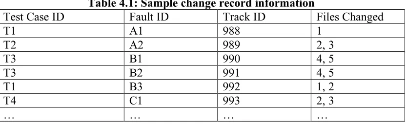
Table 4.1: Sample change record information

Test Case ID Fault ID Track ID Files Changed

T1 A1 988 1

T2 A2 989 2, 3

T3 B1 990 4, 5

T3 B2 991 4, 5

T1 B3 992 1, 2

T4 C1 993 2, 3

… … … …

We have built an example analysis matrix M, shown below in Equation 4.1 using the data from Table 4.1 and additional change records. Thus, File 2 has appeared in a track 10 times together with File 1, 21 times together with File 3, and 0 times by itself (since M(2,2) = M(2,1) + M(2,3)). Similarly, File 3 has changed 21 times with File 2 and 3 times by itself.

! ! ! ! ! ! " # $ $ $ $ $ $ % & = 17 12 0 0 0 12 15 0 0 0 0 0 24 21 0 0 0 21 31 10 0 0 0 10 25 5 4 3 2 1 5 4 3 2 1 F F F F F M F F F F F (4.1)

Upon initial examination of this matrix, we note that Files 4 and 5 change together or by themselves. Based on this, it appears that Files 4 and 5 are strongly linked in isolation from the rest of the system. Similarly, Files 1, 2, and 3 are also linked, with Files 2 and 3 having the strongest bond of the three.

4.2.6 SDAA STEP 6: PERFORM SVD ON MATRIX M

(48)

determined by the frequency of time the files changed together. A SVD of M (Equation 4.1) provides the following matrices, shown in Equations 4.2 and 4.3:

!

"

#

$

%

&

'

=

68

.

0

74

.

0

that association cluster as to its degree of participation. For example, the first association cluster is primarily composed of File 2 and File 3 due to their higher values. File 1 is a minor participant in this association cluster. If we reexamine the original analysis matrix M, we can see the strong correlation between Files 2 and 3 with a somewhat looser correlation with File 1, since these files only tend to change together and not at all with Files 4 and 5. The association cluster in the second column portrays the next most significant cluster, comprised of Files 4 and 5.

The singular values of these clusters found in the S matrix provide some indication as to how they should be analyzed. The first cluster represents 45% of the overall variability in the matrix, which can be determined by dividing the first singular value by the sum of all the singular values. The second cluster represents 25% of the overall variability. Further, the third cluster represents 22% and the fourth represents 4%. These percentages show that the first cluster defines the majority of the information regarding these files. Clusters three and four are, in effect, sub-clusters of the first cluster because they contain a similar set of files. At this step in our technique, the matrix U can provide information about the likelihood of a change in an association cluster based upon previous change information.

4.2.8 SDAA STEP 8: APPLYING THE CLUSTERS TO THE ANALYSIS GOAL

(51)

most likely files to be affected by this change. Further, the magnitude of the corresponding singular value in S indicates which cluster has churned more within the data set under examination. If the files in a new track do not all appear in the same cluster, then they represent a new execution path through the system. In this instance, files that are associated with each changed file separately can possibly be affected by this change. Finally, the files may have never changed before within the data set that was used to build the U matrix. In this instance, no historical evidence exists as to how these files may affect the system, and a new association cluster is will form to represent this new set of changes in a future analysis.

This technique is similar to the cluster rank algorithm used by Osinski et al. in their SVD-based search term clustering algorithm [38]. Osinski multiplied their document matrix by a modified U matrix from the SVD to derive the impact that each search term had on a given document. In this fashion, the values from the result vector were used to assign a document to its closest-matching search term cluster [38].

4.2.9 LIMITATIONS

(52)

would be a developer that is repairing a fault in the system and then also makes an additional change to the system and then checks all the changed code in together on the same failure report. Excessive opportunistic changes can have an adverse affect on the ability of the SVD to identify related system components because the extra opportunistic changes artificially inflate the strength of the relationship between components when in actuality the link is much weaker.

Another limitation is that our technique is not guaranteed to be safe. If there is no historical data regarding a set of files, our technique cannot provide guidance as to where the effects may be. However, our technique may be more practical for a system with a large percentage of non-executable files. Dynamic techniques might not be able to find the same dependencies that our technique finds among these files since dynamic techniques operate primarily on source files.

(53)

4.3 INDUSTRIAL FEASIBILITY STUDY

We performed a feasibility study on the use of singular value decomposition with change records to identify related system files on a large, industrial software system at IBM in Durham, NC. In this section, we will discuss our methods in conducting this feasibility study and how our results compare to actual system file relationships as determined by system experts.

4.3.1 FEASIBILITY STUDY SETUP

We selected Matlab 7.2 R2006a as our SVD tool and began by examining available data sources. IBM’s source control and fault management system generates detailed logs on tracks. The project that was selected had three consecutive minor releases. A minor release

contains small updates to functionality and fault fixes; a major release includes a significant change in functionality. Each release of the project contained approximately 21,000 files with over one million lines of code. To protect proprietary information, we cannot provide the quantity of change records analyzed.

4.3.2 CLUSTER IDENTIFICATION

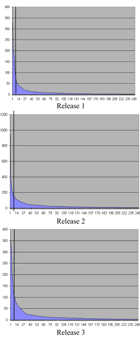
The goal of the feasibility study was to determine if the association clusters produced by SVD are intuitively identifiable by system experts and thus represent actual system

(54)

followed a parallel approach to previous research to qualitatively assess the accuracy of the clustering algorithm.

(55)

Release 1

Release 2

Release 3

(56)

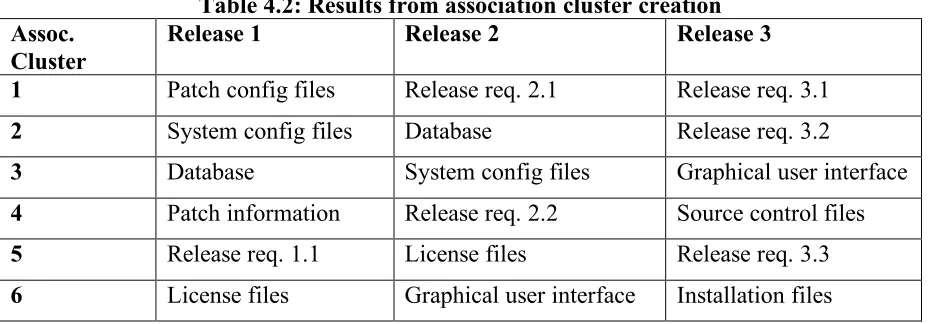
The two authorities on the system independently provided similar names for each cluster. The identifications and singular values for the six association clusters for each minor release are shown in Table 4.2 and are in order by singular value. Further, the main release requirements for all three releases were evidenced in the top six association clusters, indicating that the association clusters can identify system components and order them by velocity of change as indicated by the magnitude of the singular values. Another thing to note about these clusters is that approximately 83% of these clusters include files that are not source code, including license files, help files, configuration files, and images from the graphical user interface. This result indicates the importance of non-executable files in this particular project. From these results, we can surmise that association clusters generated from a SVD using change records can represent specific, feature-related sections of the code base.

Table 4.2: Results from association cluster creation Assoc.

Cluster

Release 1 Release 2 Release 3

1 Patch config files Release req. 2.1 Release req. 3.1

2 System config files Database Release req. 3.2

3 Database System config files Graphical user interface

4 Patch information Release req. 2.2 Source control files

5 Release req. 1.1 License files Release req. 3.3

6 License files Graphical user interface Installation files

4.4 INDUSTRIAL CASE STUDY

(57)

continue in this branch of research. From our experiences with the feasibility study, we were able to refine our data gathering and automate our SVD generation. We expanded our research on the same data set to now investigate how an impact analysis technique could be applied using the relationships found between files using the SVD. Our hypothesis is that a methodology based upon singular value decomposition using historical change records can

accurately surface additional files, including non-source files that may be impacted by a set of changes. In this section, we will discuss the use of our impact analysis technique and how its results compare to those of other techniques in use today.

4.4.1 CASE STUDY SETUP

We continued to use Matlab 7.2 R2006a as our SVD tool and the same data sources as our feasibility study. We first determined the size of the impact sets returned by our technique, and then we investigated the accuracy of those impact sets. We measured the size of the impact sets generated by our technique to determine how much our technique minimized the impact set. A random data splitting technique was used with the three minor releases of an industrial software system in this investigation to create our data sets. We began by randomly selecting two-thirds of the tracks for each release as the “historical data” for our training set, from which we generated a set of association clusters. The remaining one-third of the tracks were then used as our “future set,” which would simulate incoming tracks made to perform a system modification. We performed this data splitting exercise ten separate times for each release.

(58)

analysis technique by comparing the size of the impact set against that of other impact analysis techniques. A smaller impact set for a safe technique shows that there are fewer false positives while still retaining the full set of true positive results. We utilized a similar methodology to first investigate the relative reduction of the impact set.

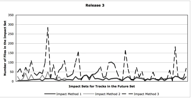
We gathered impact sets from the system modification in the future set using three different impact methods: two using our technique (Impact Methods 1 and 2) and another as a baseline (Impact Method 3):

•Impact Method 1: Gather all the files that appear in clusters in which all of the

newly-changed files appear. For example, if a new track contains files A, C, and Q, a file is considered in the impact set if it appears in a cluster in which A, C, and Q all appear together.

•Impact Method 2: Gather all the files that appear in clusters in which any of the

newly-changed files appear. For example, if a new track contains files A, C, and Q, a file is considered in the impact set if it appears in any cluster that contains at least one of files A, C, or Q.

•Impact Method 3: Gather all the files that have changed in the “historical data” with

(59)

4.4.2 CASE STUDY RESULTS

We compared the size of Impact Methods 1 and 2 impact sets to that derived by Impact Method 3. The goal of this comparison is to show that using SVD can narrow the scope of files that should be examined in the event of a system modification to those files that are most strongly connected to the changing files. An example result from Release 3 can be found in Figure 4.2.

Figure 4.2: Charts of comparisons of impact sets

(60)

After we evaluated the reduction of the size of the impact set using our technique, we investigated the accuracy of those impact sets. Because our technique generates an impact set based upon historical evidence, the files in the impact set could be considered as a recommendation for further inspection of additional files. Thus, we evaluated the accuracy of the Impact Method 1 by determining whether the files in the impact set appeared in the future set along with one of the files from the new system modification.

For the discussion of our accuracy analysis technique, consider a track in the future set that contains files A, B, and C. Impact Method 1 generates a cluster that contains A, B, C, and D, thereby providing a recommendation that D also be examined. We refer to files A, B, and C as files in the “test track” and to file D as a file in the “impact set.”

For our analysis, we considered a file in the impact set a confirmed true positive if that file appeared in any track in the future set with one or of the files from the test track. For example, if D appears in a track in the future set with either A, B, or C, we consider this matching result as a confirmed true positive. However, if D does not appear with A, B, or C in the future set, the conditions of system activity may not have involved these files. Thus, any recommendation that is not a confirmed true positive may either be an unconfirmed true positive or a false positive.

(61)

are discovered. The technique evolves along with the system itself. The results of this investigation can be found in Table 4.3.

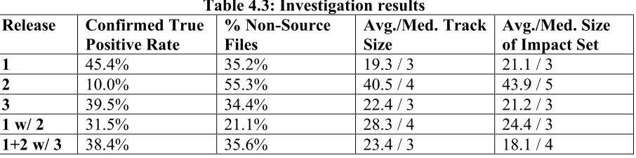
Between 21.1% and 55.3% of the files that were indicated as impacted in any given system modification were non-source files and would not have been considered in current semantic impact analysis techniques. The higher number of non-source files impacted partly the result of the type of system under investigation in this case study, but the results do indicate that often non-source files, such as images or help files, can be impacted by a system modification. Also note that the average number of impacted files is in addition to the actual changed files in the system modification.

Table 4.3: Investigation results Release Confirmed True

Positive Rate

% Non-Source Files

Avg./Med. Track Size

Avg./Med. Size of Impact Set 1 45.4% 35.2% 19.3 / 3 21.1 / 3

2 10.0% 55.3% 40.5 / 4 43.9 / 5

3 39.5% 34.4% 22.4 / 3 21.2 / 3

1 w/ 2 31.5% 21.1% 28.3 / 4 24.4 / 3

1+2 w/ 3 38.4% 35.6% 23.4 / 3 18.1 / 4

(62)

yields is a larger impact set because the SVD associates more files together, as is the case in Release 2. However, with enough information about how files change together with when the changes from Release 2 were combined with those from Release 1, the confirmed true positive rate improved because the overall change density increased.

In our background research for this work, we did not discover any other empirical analysis of an impact analysis technique that examined the accuracy of the technique based upon future system modifications. Other techniques were validated by examining the size of the impact set, given that the technique was considered safe.

4.5 OPEN SOURCE PROJECT CASE STUDY

In the previous section, we outlined our experiences with an industrial project in which we could be confident that opportunistic changes were kept to a minimum. However, there is a liklihood that some software projects