R E S E A R C H
Open Access
Analytical study of time-fractional
Navier-Stokes equation by using transform
methods
Kangle Wang
*and Sanyang Liu
*Correspondence:
[email protected] School of Mathematics and Statistics, XiDian University, Xi’an, 710118, China
Abstract
In this paper, we establish a modified reduced differential transform method and a new iterative Elzaki transform method, which are successfully applied to obtain the analytical solutions of the time-fractional Navier-Stokes equations. The obtained results show that the proposed techniques are simple, efficient, and easy to implement for fractional differential equations.
Keywords: Elzaki transform; fractional Navier-Stokes equation; reduced differential transform method
1 Introduction
In recent years, the fractional differential equations have been used in various fields such as colored noise, electromagnetic waves, boundary layer effects in ducts, viscoelastic me-chanics, diffusion processes, and so on [–]. However, most fractional differential equa-tions are very difficult to exactly solve, so numerical and approximation techniques have to be used. Recently, many powerful methods have been used to approximate linear and nonlinear fractional differential equations. These methods include the Adomain decom-position method (ADM) [, ], the homotopy perturbation method (HPM) [–], the variational iteration method (VIM) [, ], and so on.
The time-fractional Navier-Stokes equation can be written in operator form as [, ]
Dα
tu+ (u· ∇)u= –ρ∇p+v∇
u,
∇ ·u= , <α≤, (.)
whereDα
t = ∂
α
∂tα is the Caputo fractional derivative of orderα,pis the pressure,ρ is the density,uis the velocity,vis the kinematic viscosity, andtis the time. Whenα= , equation (.) is the classical Navier-Stokes equation, the form given by
ut+ (u· ∇)u= –ρ∇p+v∇u,
∇ ·u= . (.)
In this paper, we consider the unsteady flow of a viscous fluid in a tube, the velocity field is a function of only one space coordinate, the time is a dependent variable. This kind of
fractional Navier-Stokes equation has been studied by Momani and Odibat [], Kumar et al.[, ], and Khan [] by using the Adomian decomposition method (ADM), the homotopy perturbation transform method (HPTM), the modified Laplace decomposition method (MLDM), the variational iteration method (VIM), and the homotopy perturbation method (HPM), respectively.
In , Daftardar-Gejji and Jafari [] were first to propose the Gejji-Jafari iteration method for solving a linear and nonlinear fractional differential equation. The Gejji-Jafari iteration method is easy to implement and obtains a highly accurate result. The reduced differential transform method (RDTM) was first proposed by Keskin and Oturanc [, ]. The RDTM was also applied by many researchers to handle nonlinear equations arising in science and engineering. In recent years, Kumaret al.[–] used various methods to study the solutions of linear and nonlinear fractional differential equation combined with a Laplace transform.
Based on the Gejji-Jafari iteration method and RDTM, we established the new itera-tive Elzaki transform method (NIETM) and the modified reduced differential transform method (MRDTM) with the help of the Elzaki transform [, ] and we successfully ap-plied this to time-fractional Navier-Stokes equations. The results show that our proposed methods are efficient and easy to implement with less computation for fractional differ-ential equations.
2 Basic definitions
In this section, we set up notation and review some basic definitions from fractional cal-culus and Elzaki transforms.
Definition . A real functionf(x),x> , is said to be in the spaceCμ,μ∈Rif there exists
a real numberp(p>μ), such thatf(x) =xpf
(x), wheref(x)∈C[,∞), and it is said to be in the spaceCm
μ iff(m)∈Cμ,m∈N.
Definition . The Riemann-Liouville fractional integral operator of orderα≥, of a functionf(x)∈Cμ,μ≥– is defined as []
Iαf(x) =
(α) x
(x–t)
α–f(t)dt, α> ,x> ,
If(x) =f(x), α= , (.)
where(·) is the well-known Gamma function.
Definition . The fractional derivative off(x) in the Caputo sense is defined as []
Dαf(x) =In–αDnf(x) =
(n–α) x
(x–t)n–α–f(n)(t)dt, (.)
wheren– <α≤n,n∈N,x> ,f ∈Cn
–.
The following are the basic properties of the operatorDα:
() DαIαf(x) =f(x),
() IαDαf(x) =f(x) –
n–
k=
f(k)+x
Definition . The Elzaki transform is defined over the set of functions A={f(t) :
Lemma . The Elzaki transform of the Riemann-Liouville fractional integral is defined as follows[, ]:
EIαf(t) =sα+T(s). (.)
Lemma . The Elzaki transform of the Caputo fractional derivative is given as follows [, ]:
3 New iterative Elzaki transform method (NIETM)
Consider an unsteady, one-dimensional motion of a viscous fluid in a tube. The equa-tions of moequa-tions which govern the flow field in the tube are the Navier-Stokes equaequa-tions in cylindrical coordinates and they are given by [, ]
ut= –ρpz+v(urr+rur),
u(r, ) =f(r). (.)
If the fractional derivative model is used to present the time derivative term, the equation of motion (.) assumes the form
uα
t =P+v(urr+rur), <α≤,
u(r, ) =f(r), (.)
whereP= –ρpz.
Applying the Elzaki transform on both sides of equation (.), we have
Euαt =E
Using the property of the Elzaki transform and the initial condition, we get
Eu(r,t) =sf(r) +sαE
Applying the inverse Elzaki operator on both sides of (.), we obtain
We can obtain
u(r,t) =g(r,t) +Nu(r,t). (.)
The solution of equation (.) has the series form
u(r,t) = ∞
i=
ui(r,t). (.)
The operatorNcan be decomposed as
N
According to equations (.) and (.), equation (.) is equivalent to
∞
We define the recurrence relation ⎧ Similarly, for the proof of the convergence of the NIETM, see [].
4 Modified reduced differential transform method (MRDTM)
In this section, the basic definition of the modified reduced differential transform method is introduced as in [, ].
Definition . The modified reduced differential transform ofu(x,t) att=tis repre-sented as
Definition . The differential inverse transform ofUk(x,t) is represented as
According to (.) and (.), the following theorems can be obtained.
Theorem . If w(x,t) =u(x,t)±v(x,t),then MRDT[w(x,t)] =Uk(x)±Vk(x).
Applying the modified reduced differential transform on both sides of equation (.), we have
Using the property of MRDT, we can obtain
(kα+α+ )
According to equation (.), we have the following result:
U(x) =ϕ(x), U(x) =ϕ(x), U(x) =ϕ(x),
U(x) =ϕ(x), . . . .
So, we get the solution of equation (.) as follows:
5 Illustrative examples
Example Consider the following time-fractional Navier-Stokes equation:
uα
t(r,t) =P+urr(r,t) +rur(r,t),
u(r, ) = –r. (.)
5.1 Applying the NIETM
Applying the Elzaki transform on both sides of equation (.), we have
Eu(r,t) =sf(r) +sαE
P+urr+
rur
. (.)
Using the inverse Elzaki transform and the initial condition on both sides of equation (.), we get
u(r,t) =E–s –r +E–
sαE
P+urr+
rur
. (.)
Assume
g(r,t) =E–[s( –r)], N(u(r,t)) =E–[sαE[P+u
rr+rur]].
(.)
According to (.), we get the following results:
u= –r,
u=
(P– )tα
(α+ ),
u= ,
u= ,
· · ·
un= .
Therefore, the solution of equation (.) is
u(r,t) = ∞
i= ui
= –r+(P– )t
α
(α+ ). (.)
Remark . The result is the same as ADM, HPTM, HPM, and VIM by Momani and Odibat [], Kumaret al.[, ], and Khan [].
Remark . Whenα= , equation (.) is the exact solution of the classical Navier-Stokes equation as follows:
5.2 Applying the MRDTM
Applying the MRDT on both sides of equation (.), we get
MRDTuα
Using the property of MRDT, we have
(kα+α+ )
So, the solution of equation (.) is given as
u(r,t) =
Example We consider the following time-fractional Navier-Stokes equation:
uα
t(r,t) =urr(r,t) +rur(r,t), <α≤,
u(r, ) =r. (.)
5.3 Applying the NIETM
Applying the Elzaki transform on both sides of equation (.), we have
Eu(r,t) –su(r, ) –sαE
According to the initial condition, we can obtain
Eu(r,t) –sr–sαE
Using the inverse Elzaki operator on both sides of equation (.), we have
Assume
According to (.), we have the result
u=r,
Therefore, the solution of equation (.) is given as
u(r,t) =r+
Remark . The result is the same as ADM, HPTM, HPM, and VIM by Momani and Odibat [], Kumaret al.[, ], and Khan [].
Remark . Whenα= , equation (.) is the same as the exact solution of the classical Navier-Stokes equation [],
5.4 Applying the MRDTM
Applying the MRDT on both sides of equation (.), we get
MRDTuαt(r,t) =MRDTurr(r,t) +MRDT
Applying the property of MRDT, we get
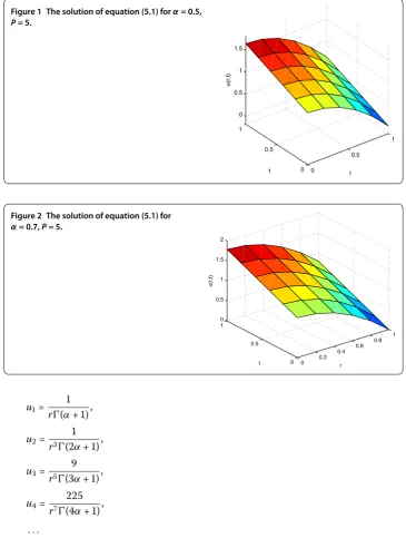
Figure 1 The solution of equation (5.1) forα= 0.5, P= 5.
Figure 2 The solution of equation (5.1) for α= 0.7,P= 5.
u= r(α+ ),
u= r(α+ ),
u= r(α+ ),
u= r(α+ ),
· · ·
un=
×× · · · ×(n– ) rn–
(nα+ ).
So, the solution of equation (.) is given as
u(r,t) = ∞
n=
Untnα=r+
∞
n=
×× · · · ×(n– ) rn–
tnα
(nα+ ). (.)
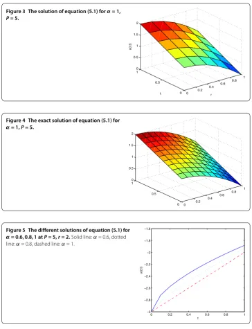
Figure 3 The solution of equation (5.1) forα= 1, P= 5.
Figure 4 The exact solution of equation (5.1) for α= 1,P= 5.
Figure 5 The different solutions of equation (5.1) for α= 0.6, 0.8, 1 atP= 5,r= 2.Solid line:α= 0.6, dotted line:α= 0.8, dashed line:α= 1.
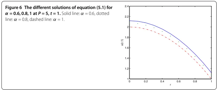
Remark . Figures -, respectively, show the approximate solution of equation (.) forα= ., ., atP= . Figure shows the exact solution of equation (.) forα= . Figure shows the different solution of equation (.) forα= ., ., atP= ,r= . Figure shows the different solution of equation (.) forα= ., ., atP= ,t= . By comparison, it is easy for us to find that the solution continuously depends on the values of the time-fractional derivative.
6 Conclusion
Figure 6 The different solutions of equation (5.1) for α= 0.6, 0.8, 1 atP= 5,t= 1.Solid line:α= 0.6, dotted line:α= 0.8, dashed line:α= 1.
Competing interests
The authors declare that they have no competing interests.
Authors’ contributions
Both authors, KW and SL, contributed substantially to this paper, participated in drafting and checking the manuscript, and have approved the version to be published.
Acknowledgements
The authors are very grateful to the editor and referees for their insightful comments and suggestions. This work was supported by the National Natural Science Foundation of China (No.: 61373174).
Received: 12 December 2015 Accepted: 8 February 2016
References
1. Oldham, KB, Spanier, J: The Fractional Calculus. Academic Press, New York (1974)
2. Kilbas, AA, Samko, SG, Marichev, OI: Fractional Integrals and Derivatives Theory and Applications. Gordon & Breach, New York (1993)
3. Hilfer, R: Application of Fractional Calculus in Physics. World Scientific, Singapore (2000)
4. Miller, KS, Ross, B: An Introduction to the Fractional Integrals and Derivatives: Theory and Application. Wiley, New York (1993)
5. Podlubny, I: Fractional Differential Equations. Academic Press, New York (1999)
6. Wazwaz, AM: A reliable modification of Adomian decomposition method. Appl. Math. Comput.102, 77-86 (1999) 7. Adomian, G: A review of the decomposition method in applied mathematics. J. Math. Anal. Appl.135, 44-501 (1988) 8. He, JH: Homotopy perturbation technique. Comput. Methods Appl. Mech. Eng.178(3), 257-262 (1999)
9. He, JH: A coupling method of a homotopy technique and a perturbation technique for nonlinear problems. Int. J. Non-Linear Mech.35, 37-43 (2000)
10. He, JH: Application of homotopy perturbation method to nonlinear wave equation. Chaos Solitons Fractals26, 695-700 (2005)
11. Ganji, DD, Sadighi, A: Application of homotopy perturbation and variational iteration methods to nonlinear heat transfer and porous media equations. J. Comput. Appl. Math.207(1), 699-708 (2007)
12. Yang, XJ, Srivastava, HM, et al.: Local fractional homotopy perturbation method for solving fractal partial differential equation. Rom. Rep. Phys.67, 752-761 (2015)
13. Safari, M, Ganji, DD, Moslemi, M: Application of He’s variational iteration method and Adomian’s decomposition method to the fractional KdV-Burgers-Kuramoto equation. Comput. Math. Appl.58, 2091-2097 (2009) 14. He, JH: A short remark on fractional variational iteration method. Phys. Lett. A375, 3362-3364 (2011)
15. Momani, S, Odibat, Z: Analytical solution of a time-fractional Navier-Stokes equation by Adomian decomposition method. Appl. Math. Comput.177, 488-494 (2006)
16. Kumar, D, Singh, J, Kumar, S: A fractional model of Navier-Stokes equation arising in unsteady flow of a viscous fluid. J. Assoc. Arab Univ. Basic Appl. Sci.17, 14-19 (2015)
17. Kumar, D, Kumar, S, Abbasbandy, S, Rashidi, MM: Analytical solution of fractional Navier-Stokes equation by using modified Laplace decomposition method. Ain Shams Eng. J.5, 569-574 (2014)
18. Khan, NA: Analytical study of Navier-Stokes equation with fractional orders using He’s homotopy perturbation and variational iteration methods. Int. J. Nonlinear Sci. Numer. Simul.10(9), 1127-1134 (2009)
19. Daftardar-Gejji, V, Jafari, H: An iterative method for solving nonlinear functional equation. J. Math. Anal. Appl.316, 753-763 (2006)
20. Keskin, Y, Oturanc, G: The reduced differential transform method for partial differential equations. Int. J. Nonlinear Sci. Numer. Simul.10(6), 741-749 (2009)
21. Keskin, Y, Oturanc, G: The reduced differential transform method for solving linear and nonlinear wave equations. Iran. J. Sci. Technol.34(2), 113-122 (2010)
22. Kumar, S, Yildirim, A, Khan, Y, Wei, L: A fractional model of the diffusion equation and its analytical solution using Laplace transform. Sci. Iran.19(4), 1117-1123 (2012)
24. Wazwaz, AM: The combined Laplace transform-Adomian decomposition method for handling nonlinear Volterra integro-differential equations. Appl. Math. Comput.216(4), 1304-1309 (2010)
25. Khan, Y, Faraz, N, Kumar, S, Yildirim, A: A coupling method of homotopy perturbation and Laplace transform for fractional models. Sci. Bull. ‘Politeh.’ Univ. Buchar., Ser. A, Appl. Math. Phys.1, 57-68 (2012)
26. Gondal, MA, Khan, M: Homotopy perturbation method for nonlinear exponential boundary Layer equation using Laplace transformation. He’s polynomials and Pade technology He’s polynomials and Pade technology. Int. J. Nonlinear Sci. Numer. Simul.11(12), 1145-1153 (2010)
27. Madani, M, Fathizadeh, M, Khan, Y, Yildirim, A: On the coupling of the homotopy perturbation method and Laplace transformation. Math. Comput. Model.53, 1937-1945 (2011)
28. Kumar, S: A new analytical modelling for fractional telegraph equation via Laplace transform. Appl. Math. Model.38, 3154-3163 (2014)
29. Elzaki, TM, Elzaki, SM: On the connections between Laplace and Elzaki transform. Adv. Theor. Appl. Math.6(1), 1-10 (2011)
30. Khalid, M, Sultana, M, Zaidi, F, Arshad, U: Application of Elzaki transform method on some fractional differential equation. Math. Theory Model.5(1), 89-96 (2015)
31. Srivastava, V, Awasthi, MK, Tamsir, M: RDTM solution of Caputo time fractional-order hyperbolic telegraph equation. AIP Adv.3(3), 032142 (2013)