Volume 2007, Article ID 57291,16pages doi:10.1155/2007/57291
Research Article
Efficient Hybrid DCT-Domain Algorithm for
Video Spatial Downscaling
Nuno Roma and Leonel Sousa
INESC-ID/IST, TULisbon, Rua Alves Redol 9, 1000-029 Lisboa, Portugal
Received 30 August 2006; Revised 16 February 2007; Accepted 6 June 2007
Recommended by Chia-Wen Lin
A highly efficient video downscaling algorithm for any arbitrary integer scaling factor performed in a hybrid pixel transform do-main is proposed. This algorithm receives the encoded DCT coefficient blocks of the input video sequence and efficiently computes the DCT coefficients of the scaled video stream. The involved steps are properly tailored so that all operations are performed using the encoding standard block structure, independently of the adopted scaling factor. As a result, the proposed algorithm offers a significant optimization of the computational cost without compromising the output video quality, by taking into account the scaling mechanism and by restricting the involved operations in order to avoid useless computations. In order to meet any system needs, an optional and possible combination of the presented algorithm with high-order AC frequency DCT coefficients discarding techniques is also proposed, providing a flexible and often required complexity scalability feature and giving rise to an adaptable tradeoffbetween the involved scalable computational cost and the resulting video quality and bit rate. Experimental results have shown that the proposed algorithm provides significant advantages over the usual DCT decimation approaches, both in terms of the involved computational cost, the output video quality, and the resulting bit rate. Such advantages are even more significant for scaling factors other than integer powers of 2 and may lead to quite high PSNR gains.
Copyright © 2007 N. Roma and L. Sousa. This is an open access article distributed under the Creative Commons Attribution License, which permits unrestricted use, distribution, and reproduction in any medium, provided the original work is properly cited.
1. INTRODUCTION
In the last few years, there has been a general proliferation of advanced video services and multimedia applications, where video compression standards, such as MPEG-x or H.26x, have been developed to store and broadcast video informa-tion in the digital form. However, once video signals are com-pressed, delivery systems and service providers frequently face the need for further manipulation and processing of such compressed bit streams, in order to adapt their char-acteristics not only to the available channel bandwidth but also to the characteristics of the terminal devices.
Video transcoding has recently emerged as a new research area concerning a set of manipulation and adaptation tech-niques to convert a precoded video bit stream into another bit stream with a more convenient set of characteristics, tar-geted to a given application. Many of these techniques allow the implementation of such processing operations directly in the compressed precoded video streams, thus offering sig-nificant advantages in what concerns the computational cost and distortion level. This processing may include changes on syntax, format, spatial and temporal resolutions, bit-rate
ad-justment, functionality, or even hardware requirements. In addition, the computational resources available in many tar-get scenarios, such as portable, mobile, and battery supplied devices, as well as the inherent real-time processing require-ments, have raised a major concern about the complexity of the adopted transcoding algorithms and of the required arithmetic structures [1–4].
In this context, spatial frame scale is often required to re-duce the image resolution by a given scaling factor (S) be-fore transmission or storage, thus reducing the output bit rate. From a straightforward point of view, image resizing of a compressed video sequence can be performed by cas-cading (i) a video decoder block; (ii) a pixel domain resizing module, to process the decompressed sequence; and (iii) an encoding module, to compress the resized video. However, this approach not only imposes a significant computational cost, but also introduces a nonnegligible distortion level, due to precision and round-offerrors resulting from the several involved compressing and decompressing operations.
described in [2,5,6]. However, despite the several different strategies that have been presented, most of such proposals are only directly applied to scaling operations using a scaling factor given by an integer power of 2 (S = 2, 4, 8, 16, etc.). Nevertheless, downscaling operations using any other arbi-trary integer scaling factor are often required. In the last few years, some proposals have arisen in order to implement these algorithms for any integer scale factors [7–11]. How-ever, although these proposals provide good video quality for integer powers of 2 scaling ratios, their performance signifi-cantly degrades when other scaling factors are applied. One other important issue is concerned with the block structure adopted by these algorithms: the (N×N) pixels block struc-ture (usually, with N = 8) adopted by most digital image (JPEG) and video (MPEG-x, H.261 and H.263) coding stan-dards requires that both the input original frame and the output downscaled frame, together with all the data struc-tures associated to the processing algorithm, are organized in (N×N) pixels blocks. As a consequence, other feasible and reliable alternatives have to be adopted in order to obtain bet-ter quality performances for any arbitrary scaling factor and to achieve the block-based organization found in most image and video coding standards.
Some authors have also distinguished the scaling algo-rithms in what concerns their output domains [12]. While the input and output blocks of some proposed algorithms are both in the DCT-domain, other approaches process encoded input blocks (DCT-domain) but provide their output in the pixel domain. The processing of such output blocks can then either continue in the pixel-domain or an extra DCT com-putation module can yet be applied, in order to recover the output of these algorithms into the DCT domain. As a con-sequence, this latter kind of approaches is often referred to as hybridalgorithms [12].
Hence, contrary to the most recent proposals [7–11], the algorithm proposed in this paper and described inSection 3 offers a reliable and very efficient video downscaling method for any arbitrary integer scaling factor, in particular, for scal-ing factors other than integer powers of 2. The algorithm is based on ahybridscheme that adopts an averaging and sub-sampling approach performed in a hybrid pixel-transform domain, in order to minimize the introduction of any inher-ent distortion. Moreover, the proposed method also offers a minimization of the computational complexity, by restrict-ing the involved operations in order to avoid spurious and useless computations and by only performing those that are really needed to obtain the output values. Furthermore, all the involved steps are properly tailored so that all operations are performed using (N×N) coefficient blocks, indepen-dently of the adopted scaling factor (S). This characteristic was never proposed before for this kind of algorithms and is of extreme importance, in order to comply the operations with most image and video coding standards and simultane-ously optimize the involved computational effort.
An optional and possible combination of the presented algorithm with high-order AC frequency DCT coefficients discarding techniques is also proposed [13–15]. These tech-niques, usually adopted by DCT decimation algorithms, pro-vide a flexible and often required complexity scalability
fea-ture, thus giving rise to an adaptable tradeoffbetween the involved scalable computational cost and the resulting video quality and bit rate, in order to meet any system require-ments.
The experimental results, presented inSection 4, show that the proposed algorithm provides significant advantages over the usual DCT decimation approaches, both in terms of the involved computational cost, the output video quality, and the resulting bit rate. Such advantages are even more sig-nificative when scaling factors other than integer powers of 2 are considered, leading to quite high peak signal-to-noise ratio (PSNR) gains.
2. SPATIAL DOWNSCALING ALGORITHMS
The several spatial-resolution downscaling algorithms that have been proposed over the past few years are usually clas-sified in the literature according to three main approaches [2,3,6]:
(i) filtering and down-sampling, which adopts a traditional digital signal processing approach, where the down-sampled version of a given block is obtained either by applying a givenn-tap filter and dropping a cer-tain amount of the filtered pixels [16]; or by follow-ing a frequency synthesis approach [17]; or by taking into account the symmetric-convolution property of the DCT [18];
(ii) averaging and down-sampling, in which every (Sx×Sy) pixels block is represented by a single pixel with its average value [5,19–22]; some approaches have even adopted optimized factorizations of the filter matrix, in order to minimize the involved computational com-plexity [20];
(iii) DCT decimation, which downscales the image by dis-carding some high-order AC frequency DCT coef-ficients, retaining only a subset of low-order terms [8,23–27]; some authors have also proposed the us-age of optimized factorizations of the DCT matrix, in order to reduce the involved computational complex-ity [25,27].
In the following, a brief overview of each of these approaches will be provided.
2.1. Pixel filtering/averaging and down-sampling approaches
From a strict digital signal processing point of view, the first two techniques may be regarded as equivalent approaches, since they only differ in the lowpass filter that is applied along the decimation process. As an example, by considering a sim-ple downscaling procedure that converts each set of (2×2) adjacent blocksbi,j (each one with (8×8) pixels) into one single (8×8) pixels blockb(seeFigure 1), these two algo-rithms can be generally formulated as follows:
b=
1
i=0 1
j=0
b0,0
(8×8) b0,1
(8×8) b1,0
(8×8) b1,1
(8×8)
2 b
(8×8)
Figure1: Downscaling four adjacent blocks in order to obtain a single block.
wherehi,j andwi,j are the considered down-sampling filter matrices.
For the particular case of the application of theaveraging approaches (usually referred to aspixel averaging and down-sampling (PAD)methods [12]), these filters are defined as [5, 19–22]
h0,0=h0,1=w0,0t=w1,0t= 1 2
u4×8 Ø4×8
,
h1,0=h1,1=w0,1t=w1,1t= 1 2
Ø4×8
u4×8
,
(2)
whereu4×8is defined as
u4×8= ⎡ ⎢ ⎢ ⎢ ⎣
1 1 0 0 0 0 0 0 0 0 1 1 0 0 0 0 0 0 0 0 1 1 0 0 0 0 0 0 0 0 1 1 ⎤ ⎥ ⎥ ⎥
⎦, (3)
and Ø4×8is a (4×8) zero matrix.
These scaling schemes can be directly implemented in the DCT-domain, by applying the DCT operator to both sides of (1) as follows:
DCT(b)=DCT 1
i=0 1
j=0
hi,j·bi,j·wi,j
. (4)
By taking into account that the DCT is a linear and orthonor-mal transform, it is distributive over matrix multiplication. Hence, (4) can be rewritten as
B=
1
i=0 1
j=0
Hi,j·Bi,j·Wi,j, (5)
whereX = DCT(x). Since theHi,j andWi,jterms are con-stant matrices, they are usually precomputed and stored in memory.
2.2. DCT decimation approaches
DCT decimation techniques take advantage of the fact that most of the DCT coefficients block energy is concentrated in the lower frequency band. Consequently, several video transcoding manipulations that have been proposed make use of this technique by discarding some high-order AC fre-quency DCT coefficients and retaining only a subset of the low-order terms. As a consequence, this approach has also
been denoted asmodified inverse transformation and decima-tion (MITD)[12] and has been particularly adopted in DCT-domain inverse motion compensation [13–15] and spatial-resolution downscaling [8,23–26] schemes.
One example of such approach was presented by Dugad and Ahuja [23], who proposed an efficient DCT decimation scheme that extracts the (4×4) low-frequency DCT coef-ficients corresponding to each of the four (8×8) original blocks (seeFigure 1). Each of these subblocks is then inverse DCT transformed, in order to obtain a subset of the original (N×N) pixels area that will represent the scaled version of the original block. The four (4×4) subblocks are then merged and combined together, in order to obtain an (8×8) pixels block.
This scheme can be formulated as follows: letB0,0,B0,1, B1,0andB1,1represent the four original (8×8) DCT coeffi -cients blocks;B0,0,B0,1,B1,0andB1,1represent the four (4×4) low-frequency subblocks ofB0,0,B0,1,B1,0, andB1,1, respec-tively;bi,j=IDCT(Bi,j), withi,j∈ {0, 1}. Then,
b=
b0,04×4 b0,14×4
b1,0
4×4
b1,1
4×4
8×8
(6)
is the downscaled version of
b=
b0,0
8×8
b0,1
8×8
b1,0
8×8
b1,1
8×8
16×16
. (7)
To computeB=DCT(b) directly fromB0,0,B0,1,B1,0, andB1,1, Dugad and Ahuja [23] have proposed the usage of the following expression:
B=C8bCt8 =CL CR C
t
4B0,0C4 Ct4B0,1C4 Ct4B1,0C4 Ct4B1,1C4
CtL CtR
=CLCt4
B0,0CLCt4 t
+CLCt4
B0,1CRCt4 t
+CRCt4
B1,0
CLCt4 t
+CRCt4
B1,1
CRCt4 t
, (8)
whereC4is the 4-point DCT kernel matrix andCLandCR are, respectively, the four left and the four right columns of C8, the 8-point DCT kernel matrix.
2.3. Arbitrary downscaling algorithms
Besides the simplest half-scaling setups previously described, many applications have arisen which require arbitrary non-integer scaling factors (S). From the digital signal processing point of view, an arbitrary-resize procedure using a scaling factorS=U/D(whereUandDmay take any nonnull rela-tive prime integer values) can be accomplished by cascading an integer upscaling module (by a factorU), followed by an integer downscaling module (by a factorD).
KS N
Discarded DCT coefficients (preprocessing)
NS=S.KS
IDCT DCT
N
Discarded DCT coefficients (postprocessing)
Figure2: Discarded DCT coefficients in arbitrary downscale DCT decimation algorithms.
Dugad, since each upsampled block will contain all the fre-quency content corresponding to its original subblocks, this approach provides better interpolation results when com-pared with the usage of bilinear interpolation algorithms.
Nevertheless, the same does not always happen in what concerns the implementation of the downscaling step using this approach, as it will be shown in the following. Mean-while, several improved DCT decimation strategies have been presented [8,24–26]. Some authors have even proposed the usage of optimized factorizations of the DCT kernel ma-trix, in order to reduce the involved computational complex-ity [25]. However, most of such proposals are only directly applied to scaling operations using a scaling factor that is a power of 2 (S = 2, 4, 8, 16, etc.). Nevertheless, downscaling operations using any other arbitrary integer scaling factors are often required. As a consequence, in the last few years proposals have arisen in order to implement DCT decima-tionalgorithms for any integer scale factor [7–11,27]. How-ever, not only are they directly influenced by the degrada-tion effect resulting from the coefficient discard, but they often suffer from computational inefficiency on their pro-cessing, either by storing a large amount of data matrices [7] or by operating with large matrices [9–11,27]. One of such proposals was recently presented by Patil et al. [27], who proposed a DCT-decimation approach based on simple ma-trix multiplications that processes each original DCT frame as a whole, without fragmenting the involved processing by the several macroblocks. However, in practical implementa-tions such approach may lead to serious degradaimplementa-tions in what concerns the processing efficiency, since the manipulation of such wide matrices may hardly be efficiently carried out in most current processing systems, namely, due to the inherent high cache missing rate that will be necessarily involved. Such degradation will be even more serious when the processing of high-resolution video sequences is considered. By using an alternative and somewhat simpler approach, Lee et al. [8] proposed an arbitrary downscaling technique by generalizing the previously described DCT decimation approach, in order to achieve arbitrary-size downscaling with scale factors (S) other than powers of 2 (e.g., 3, 5, 7, etc.). Their methodology is illustrated inFigure 2and can be described as follows:
(1) for each original block Bi,j, retain the low-frequency (KS×KS) DCT coefficientsBi,j, thus discarding the re-maining AC frequency DCT coefficients, withKS
de-fined asKS= N/S;
(2) inverse transform each subblock Bi,j to the pixel do-main, usingbi,j =CtKS(B
i,j)CKS, whereCKS is theKS -point DCT kernel matrix;
(3) concatenate (S×S) subblocks, in order to form an (NS×NS) pixels blockb, withNS defined as NS =
S·KS:
b= ⎡ ⎢ ⎢ ⎣
b0,0 · · · b0,S ..
. . .. ... bS,0 · · · bS,S
⎤ ⎥ ⎥ ⎦
(NS×NS)
; (9)
(4) computeB=DCT(b)=CNSbC t
NS, whereCNSis the NS-point DCT kernel matrix;
(5) extract the (N×N) low frequency DCT coefficients of B(withN=8), in order to obtain the (8×8) DCT-domain scaled blockB.
However, although this methodology is often claimed to provide better performance results than bilinear downscal-ing approaches in what concerns the obtained video quality [12,23], it can be shown that such statement is not always true. In particular, when these generalized DCT decimation downscaling schemes are applied using a scaling factor other than an integer power of 2, it can be shown that the obtained video quality is clearly worse than the provided by the previ-ously described pixel averaging approaches. The reason for the introduction of such degradation comes as a result of the additional DCT coefficients discarding procedure that is performed in step (5), described above (seeFigure 2). Con-trary to the first discarding step (performed in step (1)), this second discard of high-order AC frequency DCT coefficients only occurs for scaling factors other than integer powers of 2 and introduces serious block artifacts, mainly in image ar-eas with complex textured regions. To better understand such phenomenon, inTable 1it is presented the number of DCT coefficients that is considered along the implementation of this algorithm. As it can be seen, the number of discarded coefficients during the last processing step may be highly significative and its degradation effect will be thoroughly as-sessed inSection 4.
Table1: Number of DCT coefficients considered by Lee et al.’s [8] arbitrary downscaling algorithm.
Scaling factor S 2 3 4 5 6 7 8
Number of preserved coefficients in
each direction during preprocessing KS= N/S 4 3 2 2 2 2 1
Reconstructed downscaled block size NS=S·KS 8 9 8 10 12 14 8
Number of discarded coefficients in
each direction during post-processing NS−N 0 1 0 2 4 6 0
3. PROPOSED DOWNSCALING APPROACH
Considering an arbitrary integer scaling factor S = (Sx, Sy)∈ N2, whereSxandSyare the horizontal and the ver-tical down-sizing ratios, respectively, the purpose of an arbi-trary downscaling algorithm is to compute the (N×N) DCT encoded block corresponding to a set of (Sx×Sy) original blocks, each one with (N×N) DCT coefficients.
According to the previously described pixel averaging ap-proach, a generalized arbitrary integer downscaling proce-dure can be formulated as follows: by denotingbas the pixels area corresponding to the set of (Sx×Sy) original blocksbi,j, each one with (N×N) pixels,
b= ⎡ ⎢ ⎢ ⎢ ⎢ ⎢ ⎣ b0,0
b0,1
· · · b0,Sx−1
b1,0
b1,1
· · · b1,Sx−1
..
. ... . .. ...
bSy−1,0 bSy−1,1
· · · bSy−1,Sx−1 ⎤ ⎥ ⎥ ⎥ ⎥ ⎥
⎦, (10)
the downscaled (N×N) pixels block (b) can be obtained by multiplyingbwith the subsampling and filtering matricesfSx
andfSyas follows:
b=
1 SxSy
×fSy·b·f
t
Sx, (11)
wherefSqis an (N×NSq) matrix with the following structure:
fSq
(i,j)=
⎧ ⎪ ⎪ ⎨ ⎪ ⎪ ⎩
1, fori= j
Sq
, with j∈0,NSq−1
0, otherwise.
(12)
These matrices are used to decimate the input image along the two dimensions. To simplify the description, from now on it will be adopted a common scaling factor for both the horizontal and vertical directions (S=Sx=Sy). Such sim-plification does not introduce any restriction or limitation in the described algorithm. As an example, the f3 matrix (S = 3), consideringN = 5, is given by (13). This matrix may be used to perform image downscaling by a factor of 3: each set of (3×3) pixel blocks, each one composed by (5×5)
pixels, is subsampled in order to obtain a single (5×5) pixels block,
f3= ⎡ ⎢ ⎢ ⎢ ⎢ ⎢ ⎢ ⎢ ⎣
1 1 1 0 0 0 0 0 1 1 0 0 0 0 0 0 0 0 0 0 0 0 0 0 0
f0 3
0 0 0 0 0 1 0 0 0 0 0 1 1 1 0 0 0 0 0 1 0 0 0 0 0
f1 3
0 0 0 0 0 0 0 0 0 0 0 0 0 0 0 1 1 0 0 0 0 0 1 1 1 ⎤ ⎥ ⎥ ⎥ ⎥ ⎥ ⎥ ⎥ ⎦ f2 3 . (13)
However, the computation of (11) using the filtering ma-trices defined in (12) is usually difficult to handle, since it may involve the manipulation of large matrices. Further-more, although these filtering matrices may seem reasonably sparse in the pixel domain, this does not happen when this filtering procedure is transposed to the DCT domain (as it was described in the previous section), leading to the storage of a significant amount of data corresponding to these pre-computed filtering matrices. The computation of (11) is even harder to accomplish if we take into account that the (N×N) block structure adopted in image and video coding (usually withN=8) requires that the several involved operations are performed directly on blocks with (N×N) elements, which makes this approach even more difficult to be adopted.
To circumvent all these issues, a different and more ef-ficient approach is now proposed. Firstly, by splitting the fS matrix intoSsubmatricesfS0,fS1,. . .,fSS−1, each one with
(N×N) elements, the computation of (11) can be decom-posed in a series of product terms and take a form entirely similar to (1):
b= 1
S2 f 0
Sb00fS0
t
+fS0b01fS1
t
+· · ·+fS(S−1)b(S−1)(S−1)fS(S−1)
t!
(14)
or equivalently,
b= 1
S2
S−1
i=0
S−1
j=0 fi
S·bij·fSj
t
, (15)
wherebijare the several input blocks involved in the down-scaling operation, directly obtained from the input video se-quence. In the bottom of (13), it was represented the set of three (N×N)fSxsubmatrices, for the case withS =3 and N=5, withx∈[0,S−1].
of eachfSxmatrix are taken into account. In particular, it can
be shown that eachfSi ·bij·fSj
t
term only contributes to the computation of a restricted subset of pixels of the subsam-pled block (b), within an area delimited by lines ( lmin(i) :
lmax(i)) and by columns (cmin(j) :cmax(j)), where
lmin(i)=
i∗N
S
, lmax(i) =
i∗N+ (N−1) S
,
cmin(j)= j∗N
S
, cmax(j) =
j∗N+ (N−1) S
,
(16)
withi,j ∈[0,S−1]. By denoting the contribution of each blockbi,jto the sampled pixels blockbby the (nl(i)×nc(j)) matrixpi,j, one has
pi,j= fSi ·bi,j·fSj
t
nl(i)×nc(j) matrix
, (17)
wherefi
S andf
j
S are (nl(i)×N) and (nc(j)×N) matrices, respectively, withnl(i) = lmax(i)−lmin(i) + 1 andnc(j) =
cmax(j)−cmin(j) + 1, that are obtained fromfi
S andf
j
S by
only considering the lines with nonnull elements (see dashed boxes in (13)).
The resulting (N×N) pixels sampled block (b) is ob- tained by summing up the contributions of all these terms:
b= 1
S2 · S−1
i=0
S−1
j=0 pi,j
, (18)
where
pi,j
(l,c)=
⎧ ⎪ ⎪ ⎪ ⎨ ⎪ ⎪ ⎪ ⎩
pi,j, for ⎧ ⎨ ⎩l
min(i)≤l≤lmax(i),
cmin(j)≤c≤cmax(j) 0, otherwise
(19)
with 0 ≤l,c≤ (N−1). By applying such decomposition, the overall number of computations is greatly reduced, since most of the null terms of thefSmatrices are not considered
any more.
It is also worth noting that some pixels of the sampled block (b) may be obtained from several of these product-terms. Such situation will occur whenever the set ofS non-null elements of a given line of thefSmatrix is split into two
distinctfSxsubmatrices (see (13)). In such situation, the value
of the output pixel will be the sum of the mutual contribu-tion of adjacentbi,jblocks, each one with (N×N) pixels. One example of such scenario can be observed in the previously described case withS=3 andN=5 (seef3matrix in (13)) and illustrated inFigure 3. While the pixels of the first row of the sampled (N×N) output block are obtained with only the subset of blocks{b00,b01,b02}, the pixels of the second row are the result of the mutual contribution of the set of blocks{b00,b01,b02,b10,b11,b12}. The same situation can be verified in what concerns the columns of the output block: while the first column is obtained with blocks{b00,b10,b20},
p1,0
p0,2
b(0,0)
Figure3: Contributions of the several blocks of the original image (pi,j) to the final value of each pixel of the sampled blockb(S =
3,N=5).
the second column is computed with blocks{bi0,bi1}, with
i∈ {0,. . ., (S−1)}.
A particular situation also occurs whenever the original frame dimension in any of its directions is not an integer multiple ofS. In such case, the pixels of the last column (or line) cannot be obtained from theS2input pixels, since only a subset of pixels remains to be considered in that line or column. To overcome such situation, the corresponding av-eraging weights should be adjusted to the available number of pixels at the end of that line (Wc−S· Wc/S ) or column (Wl−S· Wl/S
, whereWcandWldenote the number of columns and lines of the original image. As an example, the last sampled pixel of a given line should be computed as
b
:,
Wc S
= 1
SWc−S· "
Wc/S
#×pi,Wc/S . (20)
This adjustment can be compensated a posteriori, by multi-plying the pixels of the last column of the sampled block (b) by
b
:,
Wc S
=
$
S
Wc−S· "
Wc/S #%×b
:,
Wc
S
. (21)
The same applies for the vertical direction of the sampled image.
3.1. Hybrid downscaling algorithm
As it was referred inSection 2, since the DCT is an unitary orthonormal transform, it is distributive to matrix multipli-cation. Consequently, the described scaling procedure can be directly performed in the DCT domain and still pro-vide the previously mentioned computational advantages. By considering the matrix decomposition to compute the DCT coefficients of a given pixels blockx:X=C·x·Ct, (18) can be directly computed in the DCT domain as
B=C·b·Ct= 1 S2 ·C·
S−1
i=0
S−1
j=0 pi,j
·Ct. (22)
Hybrid pixel/DCT-domain matrix composition (a) Proposed procedure
Pre-filtering
Inverse DCT
LP filtering
Sampling
S
Direct DCT (b) Equivalent approach
Figure4: DCT-domain frame scaling procedure.
account. In particular, the computation of its (nl(i)×nc(j)) nonnull elements (pi,j) can be carried out as follows:
pi,j=fSi ·bi,j·fSj
t
=fSi ·Ct·Bi,j·C·fSj
t
. (23)
By denoting the productfi
S·Ctby the (nl(i)×N) matrixFiS
and the productfSj ·Ct by the (n
c(j)×N) matrixFjS, the
above expression can be represented as
pi,j=FiS·Bi,j·FjS
t
nl(i)×nc(j) matrix
, (24)
whereBi,jis the (N×N) DCT coefficients block directly ob-tained from the partially decoded bit stream. Since all theFxS
terms (with 0≤x ≤S−1) are constant matrices, they can be precomputed and stored in memory.
The overall complexity of the described procedure can still be further reduced if the usage ofpartial DCT informa-tion[13–15] techniques is considered, as it will be shown in the following.
3.2. DCT-domain prefiltering for complexity reduction
The complexity advantages of the previously described hy-brid downscaling scheme can be regarded as the result of an efficient implementation of the following cascaded process-ing steps:inverse DCT,lowpass filtering(averaging), subsam-pling,anddirect DCT(seeFigure 4). However, the efficiency of this procedure can be further improved by noting that the signal component corresponding to most of the high-order AC frequency DCT coefficients, obtained from the first im-plicit processing step (inverse DCT), is discarded as the result of the second step (lowpass filtering). Hence, the overall com-plexity of this scheme can be significantly reduced by intro-ducing a lowpassprefiltering stage in the inverse DCT pro-cessing step, which is directly implemented by only consider-ing a subset of the original DCT coefficients. By denotingK
as the maximum bandwidth of this lowpass prefilter, given by the highest line/column index of the considered DCT coeffi -cients, only the coefficientsB&i,j(m,n)= {Bi,j(m,n) :m,n≤
I-Initialization:
Compute and store in memory the set ofFx
Smatrices;
II-Computation:
for linS=0 to W
l
S −1
, linS+=Ndo
for colS=0 to W
c
S −1
, colS+=Ndo forl=0 to (S−1) do
forc=0 to (S−1) do
pl,c
nl×nc=
Fl S
nl×K·&Bl,c
K×K·
Fc S
t K×nc
blmin:lmax,cmin:cmax+= 1 S2
pi,jnl×nc
end for end for
[B]N×N=[C]N×N·[b]N×N·CtN×N
end for end for
Figure5: Proposed hybrid downscaling algorithm.
K}will be used for the inverse DCT operation. In practice, this prefiltering can be formulated as follows:
& Bi,j=
[I]K×K 0 0 0
·Bi,j·
[I]K×K 0 0 0
t
=
Bi,j
K×K 0
0 0
,
(25)
where [I]K×Kis the (K×K) identity matrix corresponding to the considered prefilter and [Bi,j]K×Kis a (K×K) submatrix ofBi,j, obtained by extracting the (K×K) lower-order DCT coefficients. Thus, the representative contribution ofBi,j to the output pixelspi,j(see (24)) can be obtained as
pi,j
nl(i)×nc(j)=
Fi
S
nl(i)×K·
& Bi,j
K×K·
FjS
t
K×nc(j).
(26)
By adopting this scheme, the proposed procedure pro-vides a full control over the resulting accuracy level in order to fulfill any real-time requirements, thus providing a trade-offbetween speed and accuracy. Furthermore, by considering that theBi,j matrices usually have most of their high-order AC frequency coefficients equal to zero and provided thatK
is not too small, the distortion resulting from this scheme is often negligible, as it will be shown inSection 4.
3.3. Algorithm
InFigure 5, it is formally stated the proposed hybrid down-scaling algorithm, where (linS, colS) are the block coordi-nates within the target (scaled) image; (l,c) are the coordi-nates within the set ofS2blocks being sampled; andlmin,lmax,
Table2: Comparison of the several considered downscaling approaches in what concerns the involved computational cost.
Algorithm DCT coefficents M Comparison
CPAT N 2N M(HDT)
MCPAT N∝O
1
S
DDT K 2K3
N2(S+ 1)
M(HDT)
M(DDT)∝O 1
S2
HDT K KNS(K+ 4) + 2
N3+K2S2
N2S2 1
To evaluate the computational complexity of the propos-ed algorithm, the number of multiplications (M) requirpropos-ed to process each of the (Wc×Wl) pixels of the original frame was considered as the main figure of merit. Furthermore, to assess the provided computational advantages, the following different downscaling algorithms were also considered and their computational costs were evaluated, as fully described in the appendix section:
(i) cascaded pixel averaging transcoder(CPAT), as depicted in Figure 4(b), where the filtering and sub-sampling processing steps are entirely implemented in the pixel domain, by firstly decoding the whole set of DCT co-efficients received from the incoming video stream; (ii) DCT decimation transcoder(DDT) for arbitrary integer
scaling factors, as formulated by Lee et al. [8] and de-scribed inSection 2.3;
(iii)hybrid downscaling transcoder(HDT), corresponding to the proposed algorithm.
In Table 2, it is presented the obtained comparison in what concerns the involved computational cost, both in terms of the adopted scaling factor (S) and of the con-sidered number of DCT coefficients (K). This comparison clearly evidences the complexity advantages provided by the proposed algorithm when compared with other considered approaches and, in particular, with the DCT decimation transcoder (DDT). Such advantages are even more signifi-cant when higher scaling factors are considered, as it will be demonstrated in the following section.
4. EXPERIMENTAL RESULTS
Video transcoding structures for spatial downscale comprise several different stages that must be implemented in order to resize the incoming video sequence. In fact, while in INTRA-type images only the space-domain information correspond-ing to the DCT coefficients blocks has to be downscaled, in INTER-type frames the downscale transcoder must also to take into account several processing tasks, other than the de-scribed down-sampling of the DCT blocks, as a result of the adopted temporal prediction mechanism. Some of such tasks involve the reusage and composition of the decoded motion vectors, scaling of the composited motion vectors, refine-ment of the scaled motion vectors, computation of the new prediction difference obtained by motion compensation, and
so forth. All of such processing steps have been jointly or sep-arately studied in the last few years [2,3].
This manuscript focuses solely on the proposal of an efficient computational scheme to downscale the DCT co-efficients blocks decoded from the incoming video stream by any arbitrary integer scaling factor. As it was previ-ously stated, this task is a fundamental operation in most video downscaling transcoders and has been treated by sev-eral other proposals presented up to now. The evaluation of its performance was carried out by integrating the pro-posed algorithm in a reference closed-loop H.263 [28] video transcoding system, as shown inFigure 6. In this transcod-ing architecture, both the motion compensation (MC-DCT) and the motion estimation (ME-DCT) modules were imple-mented in the DCT domain. In particular, the motion esti-mation module of the encoding part of the transcoder im-plements a DCT-domain least squares motion reestimation algorithm, by considering a ±1 pixel search range [4]. By adopting such structure, the encoder loop may compute a new reduced-resolution residual, providing a realignment of the predictive and residual components and thus minimizing the involved drift [17]. Nevertheless, to isolate the proposed algorithm from other encoding mechanisms (such as motion estimation/compensation) that could interfere in this assess-ment, a first evaluation considering the provided static video quality using solely INTRA-type images was carried out in Section 4.2. An additional evaluation that also considers its real performance when processing video sequences that ap-ply the traditional temporal prediction mechanisms was car-ried out inSection 4.3.
The implemented system was applied in the scaling of a set of several CIF benchmark video sequences (Akiyo,Silent, Carphone,Table-tennis,andMobile) with different character-istics and using different scaling factors (S). Although some of the presented results were obtained using theMobilevideo sequence and a quantization setup withQ=4, the algorithm was equally assessed with all the considered video sequences and using a wide range of quantization steps, leading to en-tirely equivalent results. For all these experiments, it was con-sidered the block size (N) adopted by most image and video coding standards, withN=8 [28].
Input
VLD Q−1 +
+ 0 I
P
MC-DCT MVi
Frame memory
MVi MV
composer downscalerMV MVs
(0, 0)
P
I
DCT-domain downscaler
+
−
I
P Q VLC
MC-DCT
Output 0 I
P
Q−1
MVo
ME-DCT Memory +
+
Figure6: Integration of the proposed DCT-domain downscaling algorithm in an H.263 video transcoder.
(a) (b) (c) (d) (e)
Figure7: Space scaling of the CIFMobilevideo sequence (Q=4): (a) original frame; (b)S=2; (c)S=3; (d)S=4; (e)S=5.
(CIF) was adopted for both video sequences, by filling the re-maining area of the output frame with null pixels. By doing so, not only do the two video streams share a significant amount of the variable length coding (VLC) parameters, thus simplifying their comparison, but it also provides an easy en-coding of the scaled sequences, since their dimensions are of-ten noncompliant with current video coding standards. Nev-ertheless, only the representative area corresponding to the scaled image was actually considered to evaluate the out-put video quality (PSNR) and drift. At this respect, several different approaches could have been adopted to evaluate this PSNR performance. One methodology that has been adopted by several authors is to implement and cascade an up-scaling and a down-scaling transcoders, in order to com-pare the reconstructed images at the full-scale resolution [23]. However, since such approach also introduces a non-negligible degradation effect associated with the auxiliary up-scaling stage, it was not adopted in the presented experi-mental setup. As a consequence, the PSNR quality measure was calculated by comparing each scaled frame (obtained with each algorithm under evaluation), with a corresponding reference scaled frame, that was carefully computed in order to avoid the influence of any lossy processing step related to the encoding algorithm. An accurate quantization-free pixel filtering and down-sampling scheme was specially imple-mented for this specific purpose. This solution has proved to be a quite satisfactory alternative when compared with other possible approaches to compute the scaled reference frame (such as DCT-decimation), since it may provide a precise control over the inherent filtering process.
In the following, the proposed algorithm will be com-pared with the remaining considered downscaling algo-rithms, by considering several different evaluation metrics,
namely, thecomputational cost, thestatic video quality, the introduceddrift,and the resultingbit rate.
4.1. Computational cost
In Table 3(a), it is represented the comparison of the pro-posed HDT algorithm with the pixel-domain transcoder (CPAT) and the DCT decimation transcoder (DDT) in what concerns the involved computational complexity. As it was mentioned before, such computational cost was evaluated by counting the total amount of multiplication operations (M) that are required to implement the downscaling procedure. In order to obtain comparison results as fair as possible, all the involved algorithms adopted the same number of DCT coefficients (K) for each of these comparisons and were im-plemented for several integer scaling factors (S).
The presented results evidence the clear computational advantages provided by the proposed scheme to downscale the input video sequences by any arbitrary integer scaling factor. In particular, when compared with the DCT deci-mation transcoder (DDT), theHDTapproach presented more significant advantages for scaling factors other than integer powers of 2, leading to a reduction of the computational cost as high as 5 (S = 7). Such phenomenon was already expected and is a direct consequence of the computational inefficiency inherent to the postprocessing discarding stage of theDDTalgorithm, illustrated inFigure 2. This computa-tional advantage will be even more significant for higher val-ues of the differenceS−2log2S. The presented results also
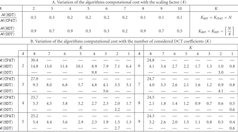
Table3: Computational cost comparison of the several considered downscaling algorithms (CIF mobile video sequence,Q=4). A. Variation of the algorithms computational cost with the scaling factor (S)
S 2 3 4 5 6 7 8 9 10 K
M(HDT)
M(CPAT) 0.5 0.3 0.2 0.2 0.2 0.2 0.1 0.1 0.1 KHDT=KCPAT=N
M(HDT)
M(DDT) 0.9 0.7 0.9 0.5 0.3 0.2 0.9 0.7 0.5 KHDT=KDDT=
'N
S
(
B. Variation of the algorithms computational cost with the number of considered DCT coefficients (K)
K K
S 8 7 6 5 4 3 2 1 S 8 7 6 5 4 3 2 1
M(CPAT) 2
30.4 — — — — — — —
6
24.8 — — — — — — —
M(HDT) 14.8 13.0 11.4 10.1 8.9 7.9 7.1 6.4 4.1 3.4 2.7 2.2 1.7 1.3 1.0 0.8
M(DDT) —- — — — 9.8 — — — — — — — — — 3.0 —
M(CPAT) 3
27.0 — — — — — — —
7
24.7 — — — — — — —
M(HDT) 9.3 8.0 6.8 5.7 4.8 4.1 3.5 3.1 4.0 3.3 2.6 2.1 1.6 1.2 0.9 0.8
M(DDT) — — — — — 5.6 — — — — — — — — 4.1 —
M(CPAT) 4
25.7 — — — — — — —
8
24.5 — — — — — — —
M(HDT) 5.3 4.5 3.8 3.2 2.7 2.3 2.0 1.7 2.1 1.8 1.4 1.2 0.9 0.7 0.6 0.5
M(DDT) — — — — — — 2.2 — — — — — — — — 0.6
M(CPAT) 5
25.2 — — — — — — —
9
24.3 — — — — — — —
M(HDT) 5.4 4.4 3.6 2.9 2.3 1.9 1.5 1.3 3.2 2.6 2.0 1.5 1.1 0.8 0.5 0.4
M(DDT) — — — — — — 2.7 — — — — — — — — 0.6
Table 3(b) presents the variation of the computational cost of the considered schemes when a different number of DCT coefficients (K) are used by the proposed algorithm to downscale the input frame using several scaling factorsS. For such experimental setups, the pixel-domain transcoder (CPAT) adopted the whole set of DCT coefficients, while the DCT decimation transcoder (DDT) adoptedK = N/S co-efficients, as defined in [8]. As it was predicted before (see Table 2), the computational cost of the proposedHDT algo-rithm significantly decreases when the number of considered DCT coefficients decreases.
The presented results also evidence a direct consequence of the computational advantage provided by the proposed algorithm: for the same amount of computations (M) and a given scaling factor (S), the proposed algorithm is able to process a greater amount of decoded DCT coefficients (K) than the DCT-decimation transcoder (DDT). This fact can be easily observed for the transcoding setup usingS=3, illus-trated inTable 3(b). By approximately using the same num-ber of operations, the DCT decimation transcoder processes onlyK2 =9 DCT coefficients of each block, while the pro-posed transcoder may processK2=25 coefficients. As it will be shown in the following, such advantage will allow this al-gorithm to obtain scaled images with greater PSNR values in transcoding systems with restricted computational resources.
4.2. Static video quality
To isolate the proposed algorithm from other processing is-sues (such as motion vector scaling and refinement, drift compensation, predictive motion compensation, etc.), a first
evaluation and assessment of the considered algorithms was performed using solely INTRA-type images. The compari-son of such static video quality performances will provide the means to better understand the advantages of the proposed approach, by focusing the attention on the most important aspects under analysis, which are the accuracy and the com-putational cost of the spatial downscaling algorithms. A dy-namic evaluation of the obtained video quality, by consider-ing the inherent drift that is introduced when temporal pre-diction schemes are applied, will be presented in the follow-ing subsection.
Table 4 presents the PSNR measure that was obtained after the space scaling operation over the Mobilevideo se-quence, considering a quantization setup withQ= 4. Sev-eral different scaling factors (S) and number of considered DCT coefficients (K) were used in these implemented se-tups. Similar results were also obtained for all the remaining video sequences and quantization steps, evidencing that the overall quality of the resulting sequences is better when the proposedHDTalgorithm is applied. These performance re-sults were also thoroughly validated by undergoing a percep-tual evaluation of the resulting video sequences using several different observers who have confirmed the obtained quality levels.
Table4: Comparison of the PSNR quality level [dB] obtained with the several considered downscaling algorithms (CIF mobile video sequence,Q=4).
K K
S 8 7 6 5 4 3 2 1 S 8 7 6 5 4 3 2 1
CPAT
2
36.0 — — — — — — —
6
36.2 — — — — — — —
HDT 36.5 36.4 35.2 31.3 31.3 24.6 21.5 18.6 36.8 36.8 36.8 36.5 36.5 34.8 32.0 24.6
DDT — — — — 31.4 — — — — — — — — — 30.2 —
CPAT
3
36.1 — — — — — — —
7
36.3 — — — — — — —
HDT 36.7 36.6 36.3 35.6 32.8 28.4 24.8 20.7 36.7 36.7 36.7 36.4 35.4 34.1 31.5 25.2
DDT — — — — — 27.9 — — — — — — — — 28.6 —
CPAT
4
36.2 — — — — — — —
8
36.3 — — — — — — —
HDT 36.7 36.6 36.6 36.0 36.0 32.5 32.5 22.0 37.0 37.0 37.0 37.0 37.0 37.0 37.0 37.0
DDT — — — — — — 32.6 — — — — — — — — 37.0
CPAT
5
36.1 — — — — — — —
9
36.3 — — — — — — —
HDT 36.7 36.7 36.5 35.9 34.8 33.8 29.5 23.6 37.0 37.0 36.9 36.6 36.0 35.4 34.2 27.0
DDT — — — — — — 28.6 — — — — — — — — 28.9
Table5: PSNR gains provided by the proposed approach over theDDTalgorithm when the number of considered DCT coefficients (K) is adjusted, so that both schemes make use of the same computational resources.
S 2 3 4 5 6 7 8 9
KDDT 4 3 2 2 2 2 1 1
KHDT 5 5 3 5 6 8 2 2
ΔPSNR −0.1 dB +7.7 dB −0.1 dB +7.3 dB +6.6 dB +8.1 dB +0.0 dB +5.3 dB
(K = N), these two algorithms actually make use of quite similar down-sampling filters. Nevertheless, by processing the incoming blocks of DCT coefficients directly in the DCT domain, the proposed algorithm reduces the total number of arithmetic operations involved in the scaling, thus reducing the inherent degradation influence of round-offand trunca-tion errors.
The second observation that is worth noting about the
HDTalgorithm is the expected decrease of the PSNR mea-sures when the number of discarded coefficients increases. Although such decrease may be negligible for greater scaling factors, its importance is highly significant for smaller scal-ings of the original image.
Finally, a careful observation should be devoted to the comparison of the performances obtained with the proposed algorithm and with the DCT decimation approach (DDT). As it was previously predicted, although both algorithms pro-vide quite similar quality performances for scaling factors given by integer powers of 2, the same does not happen when other scaling factors are considered. In such cases, the pro-posed HDTalgorithm proves to provide significantly better results than theDDTalgorithm. Moreover, by analyzing the results presented in Tables 3(b) and 4, it should be noted that such better performances are obtained with fewer op-erations. As a consequence, for downscaling operations im-plemented in restricted computational environments, where the available amount of arithmetic operations that may be carried out to process each pixel in real-time is limited, the proposed hybrid algorithm offers the possibility to process more decoded DCT coefficients than the DCT decimation
algorithm, thus potentially providing much better quality re-sults.Table 5illustrates such situation. For each scaling fac-torS, it was presented the number of DCT coefficients that are considered by the DCT decimation algorithm (DDT) as well as the number of coefficients that may be processed by the proposed hybrid algorithm (HDT), when both approaches roughly make use of the same number of operations. For each of these experimental setups, it was also presented the corresponding PSNR gain, provided by the proposedHDT ap-proach. As it can be observed, while for scaling factors given by integer powers of 2, the performances of these algorithms are quite similar (with a slight advantage for theDDT algo-rithm), for scaling factors other than integer powers of 2 and under similar computational constraints, the proposed algo-rithm is capable of providing much better quality results than the DCT decimation approach.
4.3. Drift
0 10 20 30 40 50 60 70 80 Frame
35 35.2 35.4 35.6 35.8 36 36.2 36.4
PSNR
(dB)
DDT HDT
(a) Akiyo,S=3
0 10 20 30 40 50 60 70 80
Frame 34
34.5 35 35.5 36
PSNR
(dB)
DDT HDT
(b) Akiyo,S=5
0 10 20 30 40 50 60 70 80
Frame 27
27.5 28 28.5 29
PSNR
(dB)
DDT HDT
(c) Mobile,S=3
0 10 20 30 40 50 60 70 80
Frame 27.5
28 28.5 29 29.5 30
PSNR
(dB)
DDT HDT
(d) Mobile,S=5
Figure8: PSNR obtained by downscaling theAkiyoandMobilevideo sequences, consideringQ=4 and GOP=8 frames.
Table6: Video quality (PSNR) gains provided by the proposedHDTalgorithm over theDDTapproach, for different scaling factors (S) and consideringKHDT=KDDT= N/S.
S 2 3 4 5 6 7 8
Akiyo −0.28 dB +0.19 dB −0.34 dB +0.51 dB +0.19 dB +3.68 dB −0.03 dB Silent −0.09 dB +4.29 dB −0.54 dB +8.35 dB +4.58 dB +4.17 dB −0.22 dB Carphone −0.23 dB −0.11 dB −0.28 dB +0.25 dB +1.19 dB +3.81 dB −0.10 dB Table-tennis −0.15 dB +0.34 dB −0.32 dB +1.03 dB +1.24 dB +2.32 dB −0.01 dB Mobile −0.61 dB −0.06 dB −0.36 dB +0.33 dB +1.35 dB +2.24 dB −0.10 dB
In Figure 8, it is presented the variation of the PSNR measure obtained for theAkiyoandMobilevideo sequences along the first 80 frames, when downscaled by scaling fac-tors S = 3 and S = 5 and considering a quantization parameter of Q = 4. These two video sequences feature distinct content characteristics: while the Akiyo sequence is characterized by a reduced amount of spatial and
Table7: Bit-rate gains provided by the proposedHDTalgorithm over theDDTapproach, for different scaling factors (S) and considering
KHDT=KDDT= N/S.
S 2 3 4 5 6 7 8
Akiyo −5.85% −7.05% −2.44% +1.70% −0.63% +5.40% +0.84% Silent −7.70% −10.67% −3.84% −4.05% −5.05% +0.17% −0.80% Carphone −8.67% −14.13% −4.55% −8.10% −3.70% −1.17% +2.85% Table-tennis −9.50% −13.73% −4.03% −5.14% −4.20% +0.62% −2.73% Mobile −12.30% −21.46% −7.68% −14.79% −7.68% −2.77% +1.18%
InTable 6, it is represented the average PSNR gain pro-vided by the proposed HDT approach over the DCT deci-mation scheme for several other different video sequences and scaling factors (S). Such gain was evaluated by comput-ing the average of the correspondcomput-ing PSNR difference for a time period corresponding to 300 frames. Once again, the obtained values demonstrate that while for scaling factors given by integer powers of 2, the two considered approaches provide similar quality levels (with a slight advantage for the
DDTscheme), for scaling factors other than integer powers of 2 the proposedHDTalgorithm provides significantly better quality performances. In particular, the results that were ob-tained with theSilentvideo sequence revealed a notable ad-vantage of the proposed scheme when processing this video sequence. Such advantage comes as a result of the signifi-cant amount of spatial detail that exists in the background of this sequence, which is particularly affected by the degra-dation effect introduced by the postprocessing discarding of the DCT coefficients, inherent to the DCT-decimation ap-proach. Hence, these results fully comply with the previously presented static video quality behavior.
Moreover, the charts presented inFigure 8also evidence that the effect of the inherent drift on the proposed scheme is not significantly different from the DCT-decimation ap-proach. In fact, by adopting this reference closed-loop archi-tecture (seeFigure 6) to evaluate the proposed hybrid scaling algorithm, a new reduced resolution residual is computed in the encoder loop, thus providing a realignment of the predic-tive and residual components and minimizing the involved drift [17]. Such drift mainly arises from requantization, elim-ination of some nonzero DCT coefficients and arithmetic er-rors caused by integer truncation, which will degrade the ref-erence picture used in the temporal prediction mechanism.
To compensate for this gradual degradation along the scaling process, Yin et al. [17] proposed four drift compen-sating architectures that attempt to reduce the influence of such degradation based on a drift error analysis. Although some of such proposals are mainly targeted to be applied in open-loop downscaling architectures (which are naturally more prone to the influence of this degradation), some of the presented approaches could equally be applied to the closed-loop transcoding architecture considered in this paper (e.g., Intra Refresh). However, since the main scope of this pa-per is not the actual video transcoding architecture that is adopted but it is the proposal of a computational efficient and more accurate arbitrary resizing algorithm, such com-pensation architectures were not considered. In fact, the pro-posed downscaling algorithm could equally be implemented
in the down-sample conversion modules of all architectures proposed in [17].
4.4. Bit rate
InTable 7, it is represented the average bit-rate gain provided by the proposed HDTapproach over the DCT decimation scheme for all the considered video sequences and scaling factors (S), where
Δbit-rate [%]=100×bits (HDT)−bits (DDT) bits (DDT) . (27)
As before, such gain was evaluated by averaging the diff er-ences between the amount of bits required to encode each frame by the two considered algorithms over a time pe-riod corresponding to 300 frames, considering Q = 4 and
KHDT=KDDT= N/S.
The obtained results evidence a clear advantage of the proposed algorithm over theDDTapproach, thus requiring fewer bits (up to 15% less) to encode each frame of the video sequences. Such advantage comes as a result of using a more accurate reduced-resolution reference frame, which will provide a much better temporal prediction mechanism, thus resulting in smaller residuals. In fact, the observed ad-vantage is more significative in video sequences that present greater amounts of movement, such as the Carphone, the Table-tennis,and theMobile, where such prediction mech-anism influences most the efficiency of the video encoder.
5. CONCLUSION
involved computational cost, the output video quality and the resulting bit rate. Such advantages are even more signifi-cant for scaling factors other than integer powers of 2, leading to a reduction of the computational cost as high as 5 and to quite significant PSNR gains, when compared with the usual DCT decimation techniques.
APPENDIX
COMPUTATIONAL COMPLEXITY ANALYSIS
As it was mentioned along the text, to evaluate the computa-tional complexity of the considered algorithms, the number of multiplications (M) required to process each of the (Wc×
Wl) pixels of the original frame was considered as the main figure of merit. In the following, the computational complex-ity of each algorithm will be derived.
A.1. Cascaded pixel averaging transcoder (CPAT)
In this approach (seeFigure 4(b)), the filtering and subsam-pling processing steps are entirely carried-out in the pixel domain. For each scaled block (B), most operations are performed in the computation of the S2 IDCTs, each one requiring 2N3 multiplications, since one single multiplica-tion is required to compute the average of each set of (S×S) pixels:
M(CPAT)= 1
WlWc ⎡ ⎢ ⎢ ⎢ ⎢ ⎣
WlWc
N2 ·2N 3
IDCTs
+WlWc
S2 ·1
averaging
+WlWc
S2N2 ·2N 3 DCTs ⎤ ⎥ ⎥ ⎥ ⎥ ⎦. (A.1)
By considering that 1/S2 1, it can be approximately for-mulated as
M(CPAT)≈2N. (A.2)
A.2. DCT decimation transcoder (DDT)
As it was described inSection 2.3, most operations that are required to process each scaled block (B) are performed in the computation of theS2 IDCTs, each one requiring 2K3 multiplications, and of the final (KS)-point DCT:
M(DDT)= 1
WlWc ⎛ ⎜ ⎜ ⎜
⎝WNlW2c 2K 3
IDCTs
+WlWc S2N22(KS)
3 DCT ⎞ ⎟ ⎟ ⎟ ⎠
=2K3
N2 (1 +S),
(A.3)
which can be approximately formulated as
M(DDT)≈2K3S
N2 . (A.4)
A.3. Hybrid downscaling transcoder (HDT)
To estimate the overall computational complexity of the pro-posed algorithm, one shall start by evaluating the cost of computing eachpi,jmatrix:
Mpi,j
=nl(i)KK+nl(i)Knc(j). (A.5)
Hence, it follows that
M(HDT)
= 1
WlWc ⎡ ⎢ ⎢ ⎢ ⎢ ⎢ ⎢ ⎣
WlWc S2N2
⎛ ⎜ ⎜ ⎜ ⎜ ⎜ ⎜ ⎝
S−1
i=0
S−1
j=0 Mpi,j
IDCTs + averaging + scaling + 2N3
DCTs ⎞ ⎟ ⎟ ⎟ ⎟ ⎟ ⎟ ⎠ ⎤ ⎥ ⎥ ⎥ ⎥ ⎥ ⎥ ⎦ , (A.6) where
S−1
i=0
S−1
j=0 Mpi,j
=K2S
S−1
i=0
nl(i) +K S−1
i=0
nl(i) S−1
j=0
nc(j)
.
(A.7)
By generically defining
nq=
qN+ (N−1) S − qN S
+ 1 (A.8)
as the number of lines of each fSqmatrix, it can be shown that
N≤
S−1
q=0
nq<S N S + 2 , (A.9)
where the lower limit of the previous expression corresponds to the case whenNis an integer multiple ofS, whereas the upper limit corresponds to a hypothetical worst case situa-tion when the set ofSnonnull elements of both the upper and the lower lines of each fSqmatrix are split across diff
er-ent fSqmatrices (see (13)). Thus
S−1
i=0
S−1
j=0 Mpi,j
< K2S2
N S + 2
+KS2 N S + 2 2 . (A.10)
By using the above relation, as well as (A.6), one can obtain
M(HDT)< 1
S2N2 $
K2S2 N S + 2
+KS2 N S + 2 2
+ 2N3 %
,
(A.11)
which can be approximately formulated as
M(HDT)≈KNS(K+ 4) + 2
N3+K2S2