SIMULATION OF MPC BASED SPEED CONTROL OF PERMANENT MAGNET SYNCHRONOUS MOTOR DRIVE

(1)

ENERGY EFFICIENT DOUBLE CLUSTER HEAD

SELECTION ALGORITHM FOR WSN

1_{D. SURESH,}2_{Dr. K. SELVAKUMAR}

1_{Assistant Professor, Department of Computer Science and Engineering}

Annamalai University, Annamalai Nagar, Tamilnadu, India

2_{Associate Professor, Department of Computer Science and Engineering}

Annamalai University, Annamalai Nagar, Tamilnadu, India E-mail: [email protected], [email protected]

ABSTRACT

In wireless sensor networks (WSN), the current cluster based routing techniques may result in increased network workload, energy consumption and re-transmissions. In order to overcome these issues, in this paper, we propose an energy efficient double cluster head selection algorithm for wireless sensor network. In this technique, two cluster heads namely main and sub-ordinate cluster heads are selected based on the parameters such as residual energy, minimum average distance from the member, nodes timer and node degree using particle swarm optimization technique. In this technique, each cluster member node sends the data to main cluster head. The aggregated data from the main cluster head is transmitted to sink through sub-ordinate cluster head. An energy efficient routing protocol is also developed based on the parameters expected number of retransmissions and link failure probability. By simulation results, we show that the proposed technique enhances the network lifetime and reduces the network overload.

Keywords: WSN, Cluster Based Routing, Energy Efficient, Algorithm

1. INTRODUCTION

1.1 Wireless Sensor Network

By the efficient design and implementation of wireless sensor networks, they become a burning area for researchers. A wireless sensor network is a collection of nodes and they are arranged into a cooperative network. Each node has capability of processing, multiple types of memory, have a power source, accommodate various sensors, have a RF transceiver and actuators.

A wireless sensor network (WSN) consists of spatially distributed autonomous sensors to cooperatively monitor physical or environmental conditions, such as temperature, sound, vibration pressure, motion etc. The Application domains of Wireless Sensor Network are diverse due to the availability of micro-sensors and low-power wireless communications. Wireless sensor networks (WSN) consist of a large collection of sensor nodes with each node equipped with sensors, processors and radio transceiver. Large number of sensor nodes can be deployed in a variety of situations capable of performing both military and civilian tasks owing to their low cost. [1][2][3][4]

1.2 Clustering in WSN

In WSN, the sensor nodes are grouped into self disjoint sets called a cluster. Clustering is used in WSN’s to provide network scalability, resource sharing and efficient use of constrained resources that gives network topology stability and energy saving attributes. Cluster schemes will decrease the overall energy consumption and reducing the interferences among sensor nodes. Cluster will reduce the communication overheads.

Clustering is a very effective way to reduce energy consumption in the wireless sensor networks. The total network is subdivided into smaller groups called cluster and each cluster would has a head and that is called as cluster-head (CH).

(2)

frequent topology changes, especially in a mobile environment.

1.2.1 Cluster Characteristics: Cluster has some characteristics and those are variability of cluster count, uniformity of cluster sizes, inter cluster routing and intra cluster routing.

1.2.1.1 Variability of Cluster Count: The clustering schemes are classified into two types based on variability of cluster count. Those are fixed and variable ones. In the fixed size scheme, the set of cluster-head are predetermined and the number of clusters is fixed. In the variable one scheme, the CHs are selected, randomly or based on some rules, from the deployed sensor nodes.

1.2.1.2 Uniformity of Cluster Sizes: clustering routing protocols in WSNs can be classified into two classes based on uniformity of cluster sizes. Those are even and uneven ones, respectively with the same size clusters and different size clusters in the network. Clustering with different sizes clusters is used to achieve more uniform energy consumption and avoid energy hole.

1.2.1.3 Intra-Cluster Routing: Clustering routing manners in WSNs also include two classes: single-hop intra-cluster routing methods and multiple-hop ones. For the manner of intra-cluster single-hop, all MNs in the cluster transmit data to the corresponding CH directly. Instead, data relaying is used when MNs communicate with the corresponding CH in the cluster.

1.2.1.4 Inter-Cluster Routing: Clustering routing protocols in WSNs include two classes: single-hop inter-cluster routing manners and multiple-hop ones. For the manner of inter-cluster single-hop, all CHs communicate with the BS directly. In contrast to it, data relaying is used by CHs in the routing scheme of inter-cluster multiple-hop. [5][6][7]

1.3 Double Cluster Head Selection in WSN:

The groups of clusters are mix together and choose one cluster as a cluster head. The other clusters can join on that group by sending the join request. The data should be forward through the CH to base station. The member nodes forward sensed data to CH that are processed. Clustering is very useful in reuse of bandwidth due to the node clustering and robust and scalable in the face of topological changes caused by node failure, insertion or removal.

1.3.1 Cluster-Head Characteristics:If we want to choose cluster as a cluster head then it must contain the following characteristics

1.3.1.1 Existence: clustering schemes can be grouped into two types based on the existence and the two types are cluster-head based and non-cluster-head based clustering. In the previous schemes, there exist at least one CH within a cluster, but in latest schemes there will more CHs.

1.3.1.2 Difference of Capabilities: The classification of clustering schemes in WSNs can be classified into homogeneous or heterogeneous ones. If all the sensor nodes are assigned with equal energy, computation, and communication resources and CHs are designated according to a random way or other criteria, then it will call as homogeneous schemes. In heterogeneous environment the sensor nodes are assigned with unequal capabilities, in which the roles of CHs are pre-assigned to sensor nodes with more capabilities.

1.3.1.3 Mobility: Clustering approaches in WSNs also can be grouped into mobile and stationary manners based on mobility attributes of CHs. In the former manners, CHs are mobile and membership dynamically change, thus a cluster would need to be continuously maintained. The CHs are stationary and can keep a stable cluster, which is easier to be managed. Sometimes, a CH can travel for limited distances to reposition itself for better network performance.

1.3.1.4 Role: A CH can simply act as a relay for the traffic generated by the sensor nodes in its cluster or perform aggregation/fusion of collected information from sensor nodes in its cluster. Sometime, a cluster head acts as a sink/BS that takes actions based on the detected phenomena or targets [32]. It is worth mentioning, sometimes a CH acts in more than one role.

1.4 Particle Swarm Optimization (PSO)

The particle swarm optimization algorithm was initially introduced by Kennedy and Eberhart (1995) in terms of social and cognitive behavior. This technique resolves the problems in various fields mainly in engineering and computer science.

In this technique, a group of potential elements termed as particles are initialized randomly. Each particle possesses a fitness value. The fitness value is estimated based on the fitness function to be optimized in each generation. Every deployed particle is aware of its best position (Pbi) and the

global best position (Pgi) among the particle group.

(3)

Vbi (t+1) =

))

(

))

(

)

(

t

₁

R

₁

P

ω

(1)

Qbi(t+1) = Qbi(t)+Vbi(t+1) (2)

Where V = velocity of the particle Q = position of the particle t = time

1

λ

and

λ

₂= learning factors

R1 and R2 = random numbers among 0 and 1

Pbi and Pgi = best and global position of particles

ω

= inertia weight

1.4 Problem Identification and Solution

In [15], Zhonghua Wang has proposed a novel double cluster-head routing policy based on clustering hierarchy routing. According to balancing the number of neighbor nodes, surplus energy and distance weights, it adopts first and second cluster-head mode. It will increase the overall performance of the network, decrease the cluster head energy consumption, balance energy consumption between member nodes, and prolong the entire lifetime of network. But this work didn’t consider the cluster head election time and the node degree in the selection of cluster head. Also there was no energy consumption model in this method.

In order to overcome these drawbacks, in this paper, we propose an energy efficient double cluster head selection algorithm for wireless sensor networks.

2. LITERATURE REVIEW

Da Tang et al., [11] have proposed a novel multiple cluster-heads routing protocol improved on LEACH (MCHRP). The definition of Decision Function is put forward in their algorithm according to the information of sensor nodes’ remaining energy, location and frequency once selected as cluster-heads. In MCHRP algorithm, for the first time they present the definition of Decision Function computed by information of location, remaining energy and frequency once selected as Main Cluster head, Vice Cluster-head or Alternative Cluster-head. Main Cluster-head, Vice Cluster-head and Alternative Cluster-head are decided by value of Decision Function and respectively take charge of data fusion and data transmission.

Buddha Singh et al., [12] have proposed Particle Swarm Optimization (PSO) approach for generating energy-aware clusters by optimal selection of cluster heads. The PSO eventually

reduces the cost of locating optimal position for the head nodes in a cluster. In addition, they have implemented the PSO-based approach within the cluster rather than base station, which makes it a semi-distributed method. The selection criteria of the objective function are based on the residual energy, intra-cluster distance, node degree and head count of the probable cluster heads. Furthermore, influence of the expected number of packet retransmissions along the estimated path towards the cluster head is also reflected in our proposed energy consumption model.

Levente Buttyan et al., [13] have proposed the first private cluster head election protocol. Our protocol is rather simple and it is suitable for both locations based and topology based clustering. They also proposed a useful extension to our basic protocol. While their protocol can resist against a passive observer, it is vulnerable to active attacks, in particular, to physical tampering of the nodes. More specifically, if an adversary physically compromises a sensor node, then it can learn all its state information, including the identifier of the cluster head node with which the compromised node is associated.

Zhonghua Wang et al., [15] have proposed a novel double cluster-head routing policy based on clustering hierarchy routing. According to balancing the number of neighbor nodes, surplus energy and distance weights, we adopt first and second cluster-head mode. Cluster heads are responsible for data collection and transmission respectively. This mechanism could avoid high energy consumption in single cluster head and “false” death phenomenon.

3. PROPOSED SOLUTION

3.1 Overview

(4)

3.2 Estimation of Metrics

3.2.1 Residual energy

The residual energy (Eres) of each node (Ni) after

performing one data communication is estimated using following formula. [16]

Eres = Ei – (Etx + Erx) (3)

Where Ei = Initial energy of the node

Etx & Erx = energy utilized at the time of

transmission and reception of data.

3.2.2 Distance

The minimum average distance among the sensor nodes is defined as the product of transmission range and corresponding hop counts. [17] It is given using Eq. (4)

D = Txr*HC (4)

Where Txr = transmission range

HC = hop count among the nodes.

Txr is computed using Friss free space formula

which is given below. [18]

Txr = [

rx tx

P

*

(

1 |

|

[

*

4

2

ε

β

α

π

η

−

(5)

Where

η

- operation wavelength

Ptx = Power transmitted by the sensor

Prx = Sensitivity of the receiver

α

= transmitter gain

β

= receiver gain

ε

= reflected power co-efficient of receiving antenna

3.2.3 Nodes Timer

The nodes timer is used while selecting the cluster head which is used to reduce the transmission of competing message of single node twice. Each node in the network can send the cluster head election message at time t1 or t2 which is expressed using the following equation [14]

T1 = * *τ

2 _res

ar LCH

E E T

, Eres

≥

Ear (6)

T2 =

ar res LCH

LCH _E

E T

T *

2

− , Eres < Ear (7)

LCH

T

= lasting time of electing CH and it is pre-defined

Eres = residual energy of the node

τ

= randomly generated real values distributed in the range [0.9, 1]

3.2.4 Node Degree

Node density (ND) is closely linked with the node degree which reveals the number of neighbors. It is used to find the average distance of neighbor nodes that are connected to the nodes. [19]

ND =

ς π*

_ Deg N

(8)

ς

= communication range

3.2.5 Expected number of re-transmissions

Let K is the number of links among the member nodes and cluster head. This reveals that K number of transmissions is required to deliver the packets successfully to CH.

Let PF be the link failure probability

Let O be the number of successful data delivery attempts

Probability of K successful transmission (i.e. end-to-end data delivery to CH) = (1- PF)K.

Probability of at least one unsuccessful data delivery = 1-(1- PF)K.

Hence n failure count after one successful data delivery is given by

P [O= n] = [1-(1- PF)K]n-1* (1- PF)K (9)

The expected number of re-transmissions leading to one successful data delivery is estimated using the following equation.

ERTx =

h F

P ) 1 (

1

− (10)

Where h = hop count =

K Txr

R_c

min 3

2

(11)

Rc = cluster radius

Txrmin = minimum transmission range

2Rc/3

K

= Dexp = Expected distance from

cluster member to cluster head.

3.3 Clustering

(5)

1) Swarm particles (SPi) are initialized in the

deployed network such that the particle’s position is randomly dispersed in space. Each SPi represents a search window

equivalent to the nodes position and velocity (Pi, Vi).

2) Each SPi monitors the parameters of each

node that includes the residual energy, minimum average distance from the member, nodes timer and node degree (Estimated in section 3.2.1-3.2.4)

3) Based on the monitored parameters, fitness function (Fi) of each particle is estimated

based on below Eq. (13)

res_i

f2(i) = 1/Di

f3(i) = 1/NTi

f4(i) = NDi

i.e. Fi =

)

*

(

)

/

(

)

/

(

)

*

(

4 i 3

2 1

i res

ND

NT

D

E

i i

α

+

(13)

where

α

₁,

α

₂,

α

₃and

α

₄ are weight values.

4) The local best (Pbi) and global best (Pgi)

value of fitness and position of each particles is estimated. (Described in section 1.4)

5) The position of Pbi and Pgi based on

following condition i)If Fi >Fi (Pbi)

Then

Update the position of Pbi with the fitness

value Fi

End if

ii) If Fi > Fi(Pgi)

Then

Update the position of Pgi with fitness

value Fi

End if

6) The velocity and position of each particle is updated using Eq (1) and (2)

7) The value updated in the global best particle is considered as the best value and the respective node is chosen as the main cluster head (CHM).

8) The next best global value corresponds to the sub-ordinate cluster head (CHS)

9) CHM transmits the message that contains

details about the CHM and CHS.

10) The data flow from nodes to sink occurs in the following manner

Sensor node

→

CHM

→

CHS

→

Sink

The above routing process in step 10 is explained in the forthcoming section 3.4

Figure.1.Clustering Technique

3.5 Energy Efficient Routing Protocol

In this protocol, intra and inter-cluster routes are established based on the expected number of re-transmissions and link failure probability.

Let U_REQ be the upload request message

Let U_INT be the intimation of received upload request.

Let D_Agg be the data aggregation message Let CMi be the cluster member nodes

Let DP be the data packet Let DAG be the aggregated data

1) Sink node sends a U_REQ to CHS to

upload the data collected from the sensor nodes.

Sink



U _

 →

REQ



CHSi

CHS upon receiving U_REQ transmits the

U_INT message to CHM.

CHSi

• Energy consumption is reduced

• Overhead is minimized.

• Network lifetime is increased

• The two selected cluster heads minimizes the network workload.

4. SIMULATION RESULTS

4.1 Simulation Model and Parameters

The Network Simulator (NS-2) [20], is used to simulate the proposed architecture. In the simulation, 50 mobile nodes move in a 1000 meter x 1000 meter region for 50 seconds of simulation time. All nodes have the same transmission range of 250 meters. The simulated traffic is Constant Bit Rate (CBR). In our simulation, 4 source nodes send their sensor data to the sink. We have two jamming attack nodes along the same channel.

The simulation settings and parameters are summarized in table.

Number of Nodes 50

Area Size 1000 X 1000

Mac IEEE 802.11

Transmission Range 250m Simulation Time 10,20,30,40 and

50 sec

Traffic Source CBR

Packet Size 512

Rate 100,200,300,400

and 500kb

Initial Energy 20.1J

Transmission Power 0.660

Receiving Power 0.395

4.2 Performance Metrics

The proposed Swarm Energy Efficient Double Cluster Head Selection Algorithm (EEPSO-DH) is compared with the Double cluster-head clustering algorithm using PSO (PSO-DH) technique [15]. The performance is evaluated mainly, according to the following metrics.

Packet Delivery Ratio: It is the ratio between the number of packets received and the number of packets sent.

Packet Drop: It refers the average

number of packets dropped during the transmission

Delay: It is the time taken by the nodes to

transmit the data packets to the receiver.

Energy Consumption: It is the amount of energy consumed by the nodes to transmit the data packets to the receiver.

4.3 Results

1) Based on Rate

In our first experiment we vary the transmission rate as 100,200,300,400 and 500Kb.

Rate Vs De lay

0 5 10 15 20 25

100 200 300 400 500

Rate(Kb)

D

e

la

y

(S

e

c

)

PSO-DH

[image:6.612.324.511.604.707.2]

EEPSO-DH

(7)

Rate Vs DeliveryRatio

0 0.1 0.2 0.3 0.4 0.5

100 200 300 400 500

Rate(Kb)

D

e

li

v

e

ry

R

a

ti

o

PSO-DH

EEPSO-DH

Figure 3: Rate Vs Delivery Ratio

Rate Vs Drop

0 20000 40000 60000 80000 100000

100 200 300 400 500

Rate(Kb)

P

k

ts PSO-DH

EEPSO-DH

Figure 4: Rate Vs Drop

Rate Vs EnergyConsum ption

9.5 10 10.5 11 11.5 12

100 200 300 400 500

Rate(Kb)

E

n

e

rg

y

(J

)

PSO-DH

EEPSO-DH

Figure 5: Rate Vs Energy Consumption

Rate Vs Throughput

0 5000 10000 15000

100 200 300 400 500

Rate(Kb)

T

h

ro

u

g

h

p

u

t

PSO-DH

EEPSO-DH

Figure 6: Rate Vs Throughput

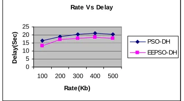
Figure 2 shows the end-to-end delay of EEPSO-DH and PSO-EEPSO-DH techniques for different transmission rate scenario. We can conclude that the end-to-end delay of our proposed EEPSO-DH approach has 13% of less than PSO-DH approach.

Figure 3 shows the delivery ratio of EEPSO-DH and PSO-DH techniques for different transmission rate scenario. We can conclude that the delivery

ratio of our proposed EEPSO-DH approach has 45% of higher than PSO-DH approach.

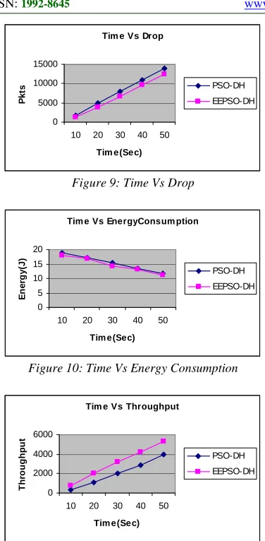
Figure 4 shows the packet drop of EEPSO-DH and PSO-DH techniques for different transmission rate scenario. We can conclude that the packet drop of our proposed EEPSO-DH approach has 13% of less than PSO-DH approach.

Figure 5 shows the energy consumption of EEPSO-DH and PSO-DH techniques for different transmission rate scenario. We can conclude that the energy consumption of our proposed EEPSO-DH approach has 4% of less than PSO-EEPSO-DH approach.

Figure 6 shows the throughput of EEPSO-DH and PSO-DH techniques for different transmission rate scenario. We can conclude that the throughput of our proposed EEPSO-DH approach has 62% of higher than PSO-DH approach.

2) Based on Time

In our second experiment we vary the simulation time as 10,20,30,40 and 50 sec.

Tim e Vs Delay

0 5 10 15 20

10 20 30 40 50

Tim e(Sec)

D

e

la

y

(S

e

c

)

PSO-DH

EEPSO-DH

Figure 7: Time Vs Delay

Tim e Vs DeliveryRatio

0 0.1 0.2 0.3 0.4 0.5

10 20 30 40 50

Tim e(Sec)

D

e

li

v

e

ry

R

a

ti

o

PSO-DH

EEPSO-DH

(8)

Tim e Vs Drop

0 5000 10000 15000

10 20 30 40 50

Tim e(Sec)

P

k

ts PSO-DH

EEPSO-DH

Figure 9: Time Vs Drop

Tim e Vs EnergyConsum ption

0 5 10 15 20

10 20 30 40 50

Tim e(Sec)

E

n

e

rg

y

(J

)

PSO-DH

[image:8.612.100.288.79.462.2]

EEPSO-DH

Figure 10: Time Vs Energy Consumption

Tim e Vs Throughput

0 2000 4000 6000

10 20 30 40 50

Tim e(Sec)

T

h

ro

u

g

h

p

u

t

PSO-DH

EEPSO-DH

Figure 11: Time Vs Throughput

Figure 7 shows the end-to-end delay of EEPSO-DH and PSO-EEPSO-DH techniques for different time scenario. We can conclude that the end-to-end delay of our proposed EEPSO-DH approach has 21% of less than PSO-DH approach.

Figure 8 shows the delivery ratio of EEPSO-DH and PSO-DH techniques for different time scenario. We can conclude that the delivery ratio of our proposed EEPSO-DH approach has 24% of higher than PSO-DH approach.

Figure 9 shows the packet drop of EEPSO-DH and PSO-DH techniques for different time scenario. We can conclude that the packet drop of our proposed EEPSO-DH approach has 17% of less than PSO-DH approach.

Figure 10 shows the energy consumption of EEPSO-DH and PSO-DH techniques for different time scenario. We can conclude that the energy consumption of our proposed EEPSO-DH approach has 5% of less than PSO-DH approach.

Figure 11 shows the throughput of EEPSO-DH and PSO-DH techniques for different time scenario. We can conclude that the throughput of our proposed EEPSO-DH approach has 38% of higher than PSO-DH approach.

5. CONCLUSION

In this paper, we have proposed an energy efficient double cluster head selection algorithm for wireless sensor network. In this technique, two cluster heads namely main and sub-ordinate cluster heads are selected based on the parameters such as residual energy, minimum average distance from the member, nodes timer and node degree using particle swarm optimization technique. When a source node wants to transmit a data to sink, energy efficient routing protocol is used based on the parameters such as the expected number of retransmissions and link failure probability. In this technique, each cluster member node sends the data to main cluster head. The aggregated data from the main cluster head is transmitted to sink through sub-ordinate cluster head. By simulation results, we have shown that the proposed technique enhances the network lifetime and reduces the network overload.

REFERENCES

[1]. John A. Stankovic, “Wireless Sensor Networks”, University of Virginia, June 19, 2006.

[2]. Mark A. Perillo and Wendi B. Heinzelman, “Wireless Sensor Network Protocols”.

[3]. F. L. LEWIS, “Wireless Sensor Networks”, Smart Environments: Technologies, Protocols, and Applications, New York, 2004.

[4]. I.F. Akyildiz, W. Su, Y. Sankarasubramaniam, and E. Cayirci, “Wireless sensor networks: a survey”, Elsevier, Page No: 393–422, 2002. [5]. Vinay Kumar, Sanjeev Jain and Sudarshan

Tiwari, “Energy Efficient Clustering Algorithms in Wireless Sensor Networks: A Survey”, International Journal of Computer Science Issues, Vol. 8, Issue 5, No 2, September 2011.

[6]. Mehdi Golsorkhtabar Amir, Naeim Rahmani and Saeed Ebadi, “FTEAP: A Fault Tolerant Energy Adaptive and Power Aware Clustering Protocol for Wireless Sensor Networks”, Journal of Global Research in Computer Science, Volume 1, No. 1, August 2010. [7]. T. Shankar, S. Shanmugavel, A. Karthikeyan

(9)

using Neural Network in Wireless Sensor Network”, European Journal of Scientific Research, 2012.

[8]. Xuxun Liu, “A Survey on Clustering Routing Protocols in Wireless Sensor Networks”, Sensors 2012.

[9]. Zohre Arabi and Roghayeh Parikhani, “Efp: New Energy–Efficient Fault-Tolerant Protocol For Wireless Sensor Network”, International Journal of Computer Networks & Communications (IJCNC) Vol.4, No.6, November 2012.

[10]. Thandar Thein, Sung-Do Chi, and Jong Sou Park, “Increasing Availability and Survivability of Cluster Head in WSN”, IEEE, 2008.

[11]. Da Tang, Xiang Liu , Yuqian Jiao and Qianjin Yue, “A Load Balanced Multiple Cluster-heads Routing Protocol for Wireless Sensor Networks”, IEEE, 2011.

[12]. 12. Buddha Singh and Daya Krishan Lobiyal, “A novel energy-aware cluster head selection based on particle swarm optimization for wireless sensor networks ”, Springer, 2012.

[13]. Levente Buttyan and Tamas Holczer, “Private Cluster Head Election inWireless Sensor Networks”, IEEE, 2009.

[14]. Feifei Li, Xi Wang and Tingrong Xu, “Energy-aware Data Gathering and Routing Protocol Based on Double Cluster-heads”, Communications in Information Science and Management Engineering, 2011.

[15]. Zhong-hua Wang, Cheng-wu Zou and Min Yu, “Double Cluster-Heads algorithm for wireless sensor networks using PSO”, International Conference on Computational and Information Sciences, 2011.

[16]. Vinh TRAN QUANG and Takumi

MIYOSHI, “Adaptive Routing Protocol with Energy efficient and event clustering for wireless sensor networks”, IEICE transactions, Vol E 91-B, No 9, 2008.

[17]. Yun Wang, Xiaodong Wang, Demin Wang and Dharma P. Agrawal, “Range-Free Localization Using Expected Hop Progress in Wireless Sensor Networks”, IEEE Transactions on Parallel and Distributed Systems, VOL. 20, NO. 10, October 2009.

[18]. Getsy S Sara, Kalaiarasi.R, Neelavathy Pari.S and Sridharan .D, “Energy efficient clustering and routing In mobile wireless sensor

network”, International Journal of Wireless & Mobile Networks (IJWMN) Vol.2, No.4, November 2010

[19]. K.Sheela Sobana Rani and Dr. N.Devarajan, “Multiobjective Sensor Node Deployement in Wireless Sensor Networks”, Vol. 4 No.04 April 2012.

[20]. Network Simulator: