Quadrotor stability using PID

QUADROTOR STABILITY USING PID

JULKIFLI BIN AWANG BESAR

A project report submitted in partial

fulfillment of the requirement for the award of the Master of Electrical Engineering

Faculty of Electrical & Electronic Engineering Universiti Tun Hussein Onn Malaysia

ABSTRACT

The quad rotor is an aerial vehicle whose motion is based on the speed of four motors. Due to its ease of maintenance, high maneuverability, vertical takeoff and landing capabilities (VTOL), etc., it is being increasingly used. The constraint with the quad rotor is the high degree of control required for maintaining the stability of the system. It is an inherently unstable system. There are six degrees of freedom – translational and rotational parameters. These are being controlled by 4 actuating signals. The x and y axis translational motion are coupled with the roll and pitch. Thus we need to constantly monitor the state of the system, and give appropriate control signals to the motors. The variation in speeds of the motors based on these signals will help stabilize the system. The unbalanced problem is one of the major

TABLE OF CONTENTS

ACKNOWLEDGEMENT i

TABLE OF CONTENTS ii

ABSTRACT iv

CHAPTER 1 INTRODUCTION 1

1.1 Overview 2

1.2 Problem Statement 2

1.3 Objective 2

1.4 Project Scope 3

1.5 Definition of Terminology 3

CHAPTER 2 LITERATURE REVIEW 4

2.1 Concepts Of Quad Rotor 4

2.1.1 Throttle 6

2.1.2 Roll 6

2.1.3 Pitch 7

2.1.4 Yaw 8

2.2 Quadcopter Model 9

2.2.1 Control System 12

2.2.2 DraganFlyer 13

2.2.3 X4-Flyer 14

2.2.4 STARMAC 15

2.3 Mathematical Analysis Of The Quad Rotor UAV 12

2.3.1 Translational Motion 18

2.3.2 Rotational Motion 18

2.4.1 State Space Equations 19

2.4.2 Linearization 19

2.5 Single Input Single Output (SISO) approach 22

CHAPTER 3 METHODOLOGY 23

3.1 Quad-Rotor Mathematical Model 23

3.2 PID Controller Development 24

3.3 Enhancement 26

CHAPTER 4 IMPLEMENTATION 28

4.1 Quad rotor simulation 28

4.2 SIMULINK Model 28

4.2.1 Controller Block 28

4.3 PWM Signal Generation Block 29

4.4 Motor Dynamics Block 31

4.5 Quad Rotor Block 32

4.6 Other SIMULINK Approach 33

4.6.1 Vertical Trust 35

4.6.2 Pitching and Rolling Moments 37

4.6.3 Yawing Moment 39

CHAPTER 5 CONCLUSION 42

5.1 Work Completed 42

5.2 Future Work 42

REFERENCES 44

CHAPTER 1

INTRODUCTION

1.1 Overview

The quad-rotor is an aerial vehicle with four motor with lift-generating propellers mounted on it. The motor was generating with spinning two propellers in clockwise and two others in counter-clockwise with all the propellers axes of rotation are fixed and parallel. The configuration of opposite pair’s directions removes the need for a

tail rotor that commonly use in standard helicopter structure.

An effective autonomous quad-rotor would have many applications such locating fire and avalanche victims to surveillance and military. The advantages to developing an autonomous quad-rotor are various and make it a worthy research topic. These belong to the so-called UAVs - VTOL (Vertical Take Off and Landing)[6], which generally are used in different areas and social approaches .The big challenge with the quad rotor is the high degree of control required for maintaining the stability of the system.

It is an inherently unstable system. There are six degrees of freedom – translational and rotational parameters[4]. These are being controlled by 4 actuating signals. The x and y axis translational motion are coupled with the roll and pitch. Thus we need to constantly monitor the state of the system, and give appropriate control signals to the motors. The variation in speeds of the motors based on these signals will help stabilize the system.

motors themselves and the electronic components associated with quad rotor control. An optimum quad-rotor design using light and strong materials can help reduce the weight of the quad-rotor. This will be one of the challenges faced during the course of the project. The hardware assembly should also be as accurate as possible to avoid any vibrations which will affect the sensors. This will make the control system perform more effectively. The complexity in the control system of the quad-rotor is accounted for in the minimal mechanical complexity of the system. As 4 small rotors are being used instead of one big rotor, there is less kinetic energy and thus, less damage in case of accidents. There is also no need of rotor shaft tilting.

1.2 Problem Statement

The unbalanced problem is one of the major problems for quad-rotor. The quad-rotor balance stability will disturb in case the disturbance exist such direct on it like a high wind speed or during outdoor flight. To overcome that problem, in this project will implement the PID controller for improving the quad-rotor self-balancing system. The aim of this development is to give a contribution in field of UAV and control system.

1.3 Objective

The goal of this project is to develop simulation control system stability for the quad rotor using a Matlab. The control scheme must enable the quad-rotor to perform stability during hovering position in rough condition (outdoor and high speed wind).

It’s can be list as:

stability in hovering condition.

2) To derive the mathematical model of quad-rotor.

3) To perform basic translational motion while maintaining stability. 4) To simulate and analyze the performance of the designed controller.

1.4 Project Scope

1) The control system design and simulation are implemented using Matlab Simulink .

2) The controller develops for improving Quad rotor stability with PID controller

1.5 Definition of Terminology

CHAPTER 2

LITERATURE REVIEW

2.1 Concepts of Quad Rotor

The quad-rotor is very well modeled with a four rotors in a cross configuration. This cross structure is quite thin and light, however it shows robustness by linking mechanically the motors (which are heavier than the structure). Each propeller is connected to the motor through the reduction gears. All the propellers axes of rotation are fixed and parallel [11][5]. Furthermore, they have fixed-pitch blades and their air flow points downwards (to get an upward lift). These considerations point out that the structure is quite rigid and the only things that can vary are the propeller speeds.

In this section, neither the motors nor the reduction gears are fundamental because the movements are directly related just to the propellers velocities. The others parts will be taken into account in the following sections. Another neglected component is the electronic box. As in the previous case, the electronic box is not essential to understand how the quad-rotor flies. It follows that the basic model to evaluate the quad-rotor movements it is composed just of a thin cross structure with four propellers on its ends.

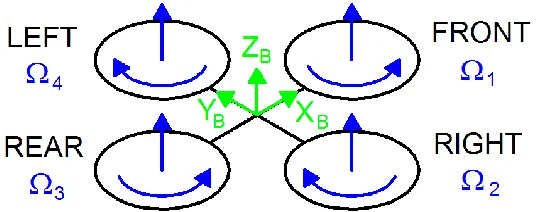
In figure 2.1 a sketch of the quad-rotor structure is presented in black. The fixed-body B-frame is shown in green and in blue is represented the angular speed of the propellers. In addition to the name of the velocity variable, for each propeller, two arrows are drawn: the curved one represents the direction of rotation; the other one represents the velocity.

Figure 2.1: Simplified quad-rotor motor in hovering

This last vector always points upwards hence it doesn’t follow the right hand rule

(for clockwise rotation) because it also models a vertical thrust and it would be confusing to have two speed vectors pointing upwards and the other two pointing downwards.

2.1.1 Throttle

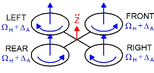
This command is provided by increasing (or decreasing) the entire propeller speeds by the same amount. It leads to a vertical force WRT body-fixed frame which raises or lowers the quad-rotor. If the helicopter is in horizontal position, the vertical direction of the inertial frame and that one of the body-fixed frame coincide.

Otherwise the provided thrust generates both vertical and horizontal accelerations in the inertial frame. Figure 2.2 shows the throttle command on a quad-rotor sketch.

Figure 2.2: Throttle motion

In blue it is specified the speed of the propellers which, in this case, is equal to ΩH + ∆A for each one. ∆A [rad s−1] is a positive variable which represents an

increment respect of the constant ΩH. ∆A can’t be too large because the model

would eventually be influenced by strong non linearity or saturations.

2.1.2 Roll

approximation)[10]. Figure 2.3 shows the roll command on a quad-rotor sketch.

The positive variables ∆A and ∆B [rad s−1] are chosen to maintain the vertical thrust unchanged. It can be demonstrated that for small values of ∆A, ∆B ≈ ∆A. As in the previous case, they can’t be too large because the model would

eventually be influenced by strong non linearities or saturations.

Figure 2.3: Roll motion

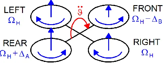
2.1.3 Pitch

This command is very similar to the roll and is provided by increasing (or decreasing) the rear propeller speed and by decreasing (or increasing) the front one [10]. It leads to a torque with respect to the yB axis which makes the quad-rotor turn.

The overall vertical thrust is the same as in hovering; hence this command leads only to pitch angle acceleration (in first approximation).

Figure 2.4 shows the pitch command on a quad-rotor sketch. As in the previous case, the positive variables ∆A and ∆B are chosen to maintain the vertical thrust

unchanged and they can’t be too large. Furthermore, for small values of ∆A, it occurs ∆B ≈ ∆A.

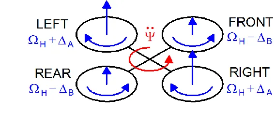
2.1.4 Yaw

This command is provided by increasing (or decreasing) the front-rear propellers’ speed and by decreasing (or increasing) that of the left-right couple. It leads to a

torque with respect to the zB axis which makes the quadrotor turn. The yaw

movement is generated thanks to the fact that the left-right propellers rotate clockwise while the front-rear ones rotate counterclockwise. Hence, when the overall

torque is unbalanced, the helicopter turns on itself around zB. The total vertical thrust

is the same as in hovering; hence this command leads only to a yaw angle acceleration (in first approximation).

Figure 2.5: Yaw motion

Figure 2.5 shows the yaw command on a quad-rotor sketch. As in the previous two cases, the positive variables ∆A and ∆B are chosen to maintain the vertical thrust unchanged and they can’t be too large. Furthermore it maintains the

2.2 Quadcopter model

Figure 2.6 : All of the States (b stands for body and e stands for earth)

Based on figure 2.6 ,it can be modelling as where below,

U1 = sum of the thrust of each motor

Th1= thrust generated by front motor

Th2= thrust generated by rear motor

Th3= thrust generated by right motor

Th4= thrust generated by left motor

m = mass of Quadcopter g = the acceleration of gravity

l = the half length of the Quadcopter x, y, z = three position

θ, ɸ, ψ = three Euler angles representing pitch, roll, and yaw

The mathematical design to move Quadcopter from landing position to a fixed point in the space is shows [1] in Equation (3.1).

(2.1)

R = matrix transformation

= Sin (θ), = Sin (ɸ), = Sin (ψ) = Cos (θ), = Cos (ɸ), = Cos (ψ)

The equations of motion can be written using the force and moment balance as shown in Equation (3.2) to Equation (3.4).

= u1 (CosɸSinθCosψ + SinɸSin) – K1ẋ/m (2.2)

= u1 (SinɸSinθCosψ + CosɸSin) – K2ẏ/m (2.3)

= u1 (CosɸCosψ) -g – K3 /m (2.4)

Where,

Ki = drag coefficient (Assume zero since drag is negligible at low speed)

From the Equation (2.2) to Equation (2.4), Pythagoras theorem can compute as Figure 2.6.

From the Figure 2.7, the Phi (ɸd) and Psi (ψd) can be extracted in the following

expressions

ɸd =

(2.5)

ψd =

(2.6)

Quadcopter have four input forces that are U1, U2, U3, and U4. This four

controller’s input will affects certain side of Quadcopter. U1 affect the attitude of the

Quadcopter, U2 affects the rotation in roll angle, U3 affects the pitch angle and U4

control the yaw angle. These four inputs force will control the Quadcopter movement. The equations of these inputs are shown in Equation (2.7).

U1 = (Th1 + Th2 + Th3 + Th4) / m

U2 = l (-Th1-Th2+Th3+Th4) / I1

U3 = l (-Th1+Th2+Th3-Th4) / I2

U4 = l (Th1+Th2+Th3+Th4) / I3 (2.7)

Where,

Thi = thrust generated by four motor

C = the force to moment scaling factor

Ii = the moment of inertia with respect to the axes

Therefore the Equation of Euler angles become:

= U2 – lK4 /I1 (2.8)

= U3– lK5 /I2 (2.9)

= U1– lK6 /I3 (2.10)

2.2.1 Control System

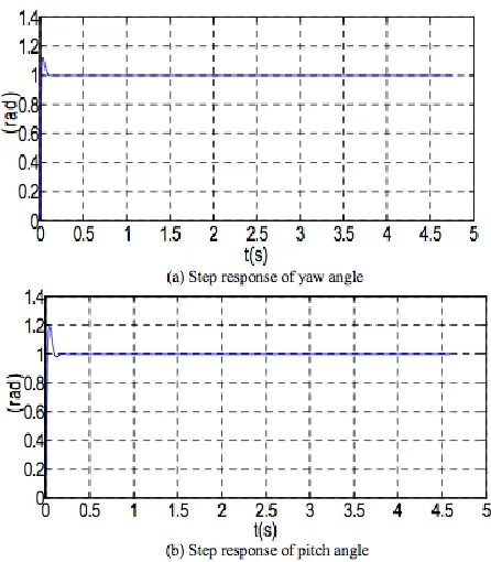
Jun Li et.al. [2] is done research to Dynamic Analysis and PID Control quad-rotor. This paper is describe the architecture of Quadrotor and analyzes the dynamic model on it based on PID control scheme [1]. Simulink model of PID controller and flying result done in this research are show in Figure 2.8 and Figure 2.9.

Figure 2.8: Simulink model of PID controller block

In the research its using a conventional schemes of PID control for make the dynamic self-balancing. The system overshoot is small, at the same time the steady-state error is almost zero, and the system response is fast. In the PID design some modification can be done to make it more effectiveness and eliminates some constrainess of conventional PID ( will describe in chapter 3) .

Some controller use PI method incorporating with compensation to correct the error present between the reference vectors and the rotational matrix’s previous

calculation. The Proportional, Integral that more simplify of code [2] . The derivative is difficult to implement on the microcontroller, both in use of resources and coding the algorithm.

Figure 2.10: PI controller for mitigating gyro drift

2.2.2 DraganFlyer

The first quad-rotor was invented in 1907 by French, Breguet Brothers with named Gyroplane No.1 . Then in 1922 Georges de Bothezat come out with a rotor located at each end of a truss structure of intersecting beams, placed in the shape of a cross .

Figure 2.11: Quadrotor designed in Pennsylvania State University.

One camera placed on the ground captures the motion of five 2.5 cm colored markers present underneath the DraganFlyer, to obtain pitch, roll and yaw angles and the position of the quadrotor by utilizing a tracking algorithm and a conversion routine. In other words, two-camera method has been introduced for estimating the full six degrees of freedom (DOF) pose of the helicopter. Algorithm routines ran in an off board computer. Due to the weight limitations GPS or other accelerometers could not be add on the system. The controller obtained the relative positions and velocities from the cameras only.

Two methods of control are studied – one using a series of mode-based, feedback linearizing controllers and the other using a back-stepping control law. The helicopter was restricted with a tether to vertical, yaw motions and limited x and y translations. Simulations performed on MATLAB-Simulink show the ability of the controller to perform output tracking control even when there are errors on state estimates.

2.2.3 X4-Flyer

receiver allowing direct plot input from a JP 3810 radio transmitter and has two separate RS232 serial channels, the first used to interface with the inertial measurement unit (IMU) and second used as an asynchronous data linked to the ground based computer.

As an IMU the most suitable unit considered was the EiMU embedded inertial measurement unit developed by the robotics group in QCAT, CSIRO weighs 50- 100g. Crossbow DMU-6 is also used in the prototype. The pilot augmentation control system is used. A double lead compensator is used for the inner loop. The setup is shown in Figure 2.11.

Figure 2.12: The X4-Flyer developed in FEIT, ANU

2.2.4 STARMAC

The base system is the off-the-shelf four-rotor helicopter called the DraganFlyer III, which can lift approximately 113,40 grams of payload and fly for about ten minutes at full throttle. The open-loop system is unstable and has a natural frequency of 60 Hz, making it almost impossible for humans to fly. An existing onboard controller slows down the system dynamics to about 5 Hz and adds damping, making it pilotable by humans. It tracks commands for the three angular rates and thrust. An upgrade to Lithium-polymer batteries has increased both payload and flight duration, and has greatly enchanced the abilities of the system.

For attitude measurement, an off-the-shelf 3-D motion sensor developed by Microstrain, the 3DM-G was used. This all in one IMU provides gyro stabilized attitude state information at a remarkable 50 Hz. For position and velocity measurement, Trimble Lassen LP GPS receiver was used. To improve altitude information a downward-pointing sonic ranger (Sodar) by Acroname were used, especially for critical tasks such as take off and landing. The Sodar has a sampling rate of 10 Hz, a range of 6 feet, and an accuracy of a few centimeters, while the GPS computes positions at 1 Hz, and has a differential accuracy of about 0.5 m in the horizontal direction and 1 m in the vertical. To obtain such accuracies, DGPS planned be implemented by setting up a ground station that both receives GPS signals and broadcasts differential correction information to the flyers.

All of the onboard sensing is coordinated through two Microchip 40 MHz PIC microcontrollers programmed in C. Attitude stabilization were performed on board at 50 Hz, and any information was relayed upon request to a central base station on the ground. Communication is via a Bluetooth Class II device that has a range of over 150 ft. The device operates in the 2.4 GHz frequency range, and incorporates bandhopping, error correction and automatic retransmission. It is designed as a serial cable replacement and therefore operates at a maximum bandwidth of 115.2 kbps. The communication scheme incorporates polling and sequential transmissions, so that all flyers and the ground station simultaneously operate on the same communication link. Therefore, the bandwidth of 115.2 kbps is divided among all flyers.

for position control. Manual flight is performed via standard joystick input to the ground station laptop. Waypoint control of the flyers was performed using Labview on the groundstation due to its ease of use and on the fly modification ability. Control loops have been implemented using simple PD controllers. The system while hovering is shown in Figure 2.13.

Figure 2.13: Quadrotor designed in Stanford University

2.3 Mathematical Analysis Of The Quad Rotor UAV

The quad rotor has six degrees of freedom that can be divided into two parts:

1) Translational – translational motion occurs in x, y, and z directions.

2) Rotational – rotational motion occurs about x, y and z directions and

named as roll (φ), pitch (θ), and yaw (ψ). 


The frames of reference used are:

1) Earth’s frame (an inertial frame of reference)

2) Body-axis (a non-inertial frame of reference) 


The model derived is based on the following assumptions:

1) The structure is rigid and symmetrical

2) The center of gravity and the body fixed frame origin coincide

3) The propellers are rigid

2.3.1 Translational Motion

In order to derive the equations representing the translation motion, the basic equation used is:

Where, ∑ represents the sum of all the external forces on the system, M is the total mass of the system
 and a is the total acceleration vector of the system.

The forces acting on the system can be devided to 2 type:

1) Thrust due to four propellers .

2) Force of gravity

And the equations obtained are:

2.3.2 Rotational Motion

In order to derive the equations representing the rotational motion, the basic equation used is:

The equations obtained are ;

2.4 Multiple Input Multiple Output (MIMO) Approach

The above 6 equations which represent the fundamental equations of the Quadrotor are coupled. To perform control the Quadrotor either a MIMO approach or a SISO approach can be made. For MIMO approach the following procedure can be followed [9].

2.4.1 State Space Equations

Now, in order to study the stability of the system the system is written in the form:

2.4.2 Linearization

The system of equations 2.1 to 2.6 are non-linear coupled equations. Therefore, the

system of equations was linearized using ‘small perturbation theorem’.

The states of the system are:

Inputs to the system are:

Equations 3.1 to 3.3 represent translational motion and equation 3.4 to 3.6 represent rotational motion. For simplification purpose, the following constants were assumed in the equations:

Perturbation is marked by the suffix ‘e’. Hence, perturbation in w is written as:

Since

where

and

Perturbation in u:

since :

so,

where,

and the state space equation was thus formed as.

The corresponding Eigen values of the A matrix was also found. and were used to obtain the matrices A and B.

2.5 Single Input Single Output (SISO) Approach

The fundamental equations are decoupled based on certain assumptions as follows :

1) The quad rotor is assumed to have very low linear and angular

velocities when in motion and assumed not to tilt beyond 15 in pitch

and roll. The quad rotor is always flying at near hovering conditions

and Coriolis and rotor moment of inertia terms can be 
 neglected.

2) Attitude is controlled by manipulating the four degrees of freedom

involved –altitude, roll, pitch and yaw.

3) The equations representing the four degrees of freedom are:

CHAPTER 3

METHODOLOGY

3.1 Quad-Rotor Mathematical Model

The dynamics of the quad-rotor is well described in the previous chapter. However the most important concepts can be summarized in equations (3.1) and (3.2). The first one shows how the quad-rotor accelerates according to the basic movement commands given.

The second system of equations show the basic movements related to the propellers’ squared speed.

3.2 PID Controller Development

A proportional integral derivative controller (PID controller) is a common method in control system. PID theory helps better control equation for the system. Some of the advantages are:

1) Simple structure.

2) Good performance for several processes,

3) Tunable even without a specific model of the controlled system.

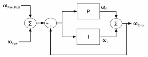
In the PID control the algorithm is various; there is no single PID algorithm. The conventional PID structures show as Figure 3.1

Figure 3.1: Block diagram of PID conventional structure.

REFERENCES

1. Jun Li, YunTang Li (2011). “Dynamic Analysis and PID Control for a Quadrotor” 2011 International Conference on Mechatronics and Automation.

2. Jared Rought, Daniel Goodhew, John Sullivan and Angel Rodriguez (2010). “Self-Stabilizing Quad-Rotor Helicopter”.

3. Pounds, P., Mahony, R., and Corke, P., “Modelling and Control of a

Quad-Rotor Robot,” In Proceedings of the Australasian Conference on Robotics and Automation, 2006.

4. Atheer L. Salih, M. Moghavvemil, Haider A. F. Mohamed and Khalaf Sallom Gaeid (2010). “Flight PID controller design for a UAV Quadcopter.”

5. Scientific Research and Essays Vol. 5(23), pp. 3660-3667, 2010.

6. Engr. M. Yasir Amir ,Dr. Valiuddin Abbass (2008). “Modeling of Quadrotor Helicopter Dynamics”. International Conference on Smart Manufacturing

Application.

7. Bouabdallah, S.; Noth, A.; Siegwart, R.; , "PID vs LQ control techniques applied to an indoor micro quadrotor," Intelligent Robots and Systems, 2004. (IROS 2004).

9. G.Hoffmann, D.Dostal, S.Waslander, J.Jang, C.Tomlin, “Stanford Testbed of Autonomous Rotorcraft for Multi-Agent Control(STARMAC) “, Stanford university, October 28th, 2004.

10.Hongxi Yang; Qingbo Geng (2011); , "The design of flight control system for small UAV with static stability," Mechanic Automation and Control Engineering (MACE), 2011 Second International Conference.

11. Claudia Mary, Luminita Cristiana Totu and Simon Konge

Koldbæk,”Modelling and Control of Autonomous Quad-Rotor”, Faculty of

Engineering, Science and Medicine University of Aalborg, Denmark (2010).