Three-Dimensional Analysis of Lateral Pile Response using Two-Dimensional Explicit Numerical Scheme

Three-Dimensional Analysis of Lateral Pile Response using

Two-Dimensional Explicit Numerical Scheme

Assaf Klar

and Sam Frydman

Abstract: A procedure for exploiting a two-dimensional共2D兲explicit, numerical computer code for the 3D formulation of dynamic lateral soil-pile interactions is considered. The procedure is applied to two models using simultaneous computation of a series of plane strain boundary value problems, each of which represents a horizontal layer of soil. The first model disregards the shear forces developed between the horizontal layers, and may be considered as a generalized Winkler model. The second model takes account of these forces by coupling the behavior of the horizontal layers. Several verification problems for a single pile and pile groups in a homogeneous soil layer modeled as a viscoelastic material were solved and compared to known solutions in order to assess the reliability of the models. Excellent agreement was observed between results of the present analyses and existing solutions.

DOI: 10.1061/共ASCE兲1090-0241共2002兲128:9共775兲

CE Database keywords: Three-dimensional analysis; Piles; Lateral loads; Dynamic loads; Pile groups; Seismic response; Soil-pile interaction.

Introduction

Many methods have been proposed for analysis of dynamic lat-erally loaded piles and pile groups. Each method has its own advantages and disadvantages; rigorous analytical methods and boundary integral methods共e.g., Tajimi 1969; Kaynia and Kausel 1982; Mamoon et al. 1988兲are restricted to viscoelastic materials and frequency domain analysis, true three-dimensional共3D兲finite element method or finite difference method analyses require sig-nificantly large calculation time, and simple Winkler models共 My-lonakis and Gazetas 1999兲have difficulty in modeling the pile-soil-pile interaction for nonlinear materials. Furthermore, most of the soil-pile interaction analysis methods require computer codes designed specifically for that purpose, some of which are com-mercial, and others research codes 关e.g., Blaney et al. 1976共the 3D finite element research code NONSPS兲; Kagawa 1983 共the beam-on nonlinear Winkler foundation research code DY NA3兲; Novak et al. 1990 共the commercial code for pile and pile groups analysis PILE-3D兲; Wu and Finn 1997a, b 共a quasi-3D finite element research code兲兴. This paper describes a procedure for utilizing explicit 2D finite element共FE兲and finite difference共FD兲 codes for representation of a 3D soil-pile interaction under static and dynamic loading. This technique was developed using the commercially available 2D geotechnical finite difference code FLAC Ver. 3.4 共Itasca 1999兲 共hereafter referred to as the FD code兲. Although the procedure is not limited to this code, its user-available, internal programming feature makes the

implementa-tion of the technique quite simple. Furthermore, no extensive knowledge of numerical methods 共creation of stiffness matrices, etc.兲is required for implementation of the technique, and thus its use is feasible for any practicing engineer. Two models were de-veloped using this technique; a generalized Winkler 共uncoupled兲 model, and a coupled model. Several verification problems of single piles and pile groups under different loading conditions were analyzed and the results were compared with known solu-tions in order to assess the reliability of the models. In these verification problems, the soil was modeled as a homogeneous, viscoelastic material. However, the models are also applicable for nonlinear constitutive models. The work presented is part of broader research; the aim of the present paper is only to introduce the approach. Consequently, nonlinear behavior is not considered here, but will be the subject of future publications.

Outline of Proposed Technique

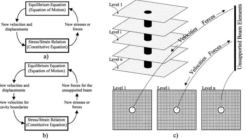
The technique is based on discretization of the 3D soil continuum into a series of horizontal layers, each layer represented by a 2D boundary value problem 共BVP兲. The initial FD grid may be di-vided into several disconnected subgrids, thus allowing the simul-taneous calculation of several BVPs. For representation of the physical problem, a cavity共or cavities in the case of a pile group兲 is inserted in each subgrid in order to model the pile cross section in that layer. Different soil properties and/or initial stresses may be introduced for each layer, as required. In addition, a separate grid consisting of a series of connected, unsupported beam ele-ments, representing the pile, is defined. In the case of a pile group with a cap, another separate subsystem should be defined to rep-resent the cap. The procedure advances in time, in correspon-dence with the FD explicit time marching calculation scheme, and develops the interaction between the two 共or three兲 systems through transfer of velocities and forces from pile共beam兲nodes to the BVP’s grid point and vice versa. In each calculation cycle 共time step兲the pile’s motion equations are solved and the veloci-ties of each pile segment’s nodes are applied to the corresponding 1_{Graduate Student, Faculty of Civil Engineering, Technion, Haifa,}

Israel.

2_{Professor, Faculty of Civil Engineering, Technion, Haifa, Israel.}

Note. Discussion open until February 1, 2003. Separate discussions must be submitted for individual papers. To extend the closing date by one month, a written request must be filed with the ASCE Managing Editor. The manuscript for this paper was submitted for review and pos-sible publication on June 26, 2001; approved on February 13, 2002. This paper is part of the Journal of Geotechnical and Geoenvironmental

Engineering, Vol. 128, No. 9, September 1, 2002. ©ASCE, ISSN

cavity boundary nodes. Next, in the same calculation cycle, the resulting forces acting on the cavity perimeter are extracted and applied to the appropriate pile segment’s nodes. These forces are then used in solving the pile’s equation of motion in the next time step, producing new velocities which are again transferred to the relevant cavity nodes. Fig. 1 demonstrates the concept of the pro-cedure. It should be realized that, by applying the pile velocities to the cavity perimeter in the same calculation cycle, a full com-patibility of displacement is achieved. This formulation describes only the interaction between the pile and the horizontal layers. The formulation of the BVP’s coupling and the consideration of seismic loading will be described later.

Uncoupled Model

A 3D soil-pile interaction problem may be solved by discretiza-tion of the soil continuum into horizontal layers, where each layer is represented by a different uncoupled plane strain problem. This technique may be classified as a generalized Winkler approach. Although it is considered approximate, its predictions are in good agreement with rigorous solutions, within some limitations. Novak共1974兲was the first to use this technique for evaluating the behavior of a single pile under lateral dynamic loading in a ho-mogenous soil layer. He used an analytical solution of the plane strain problem in conjunction with the equation of equilibrium of the pile. Novak and El-Sharnouby 共1983兲 extended these solu-tions to the case of soil properties varying with depth. Nogami and Novak共1980兲showed that, for a frequency of loading higher than the fundamental natural frequency of the system, the soil medium can be treated as a Winkler model. The uncoupled model presented herein is based on this same assumption, but it is not restricted to viscoelastic material or frequency domain analysis. Since the BVPs are uncoupled, the formulation presented in the previous paragraph needs no modification for piles laterally loaded at their heads, and only minor modification for seismic

loading. Several verification problems for different pile configu-rations and loading conditions are presented in the following sec-tions.

Uncoupled Model: Lateral Dynamic Loading of Single Pile

Neglecting the internal damping of a pile embedded in a Winkler medium, the differential equation may be written as follows 共Novak and Aboul-Ella 1978兲:

EpIp

⳵4_u共z,t兲 ⳵z4 ⫹␮

⳵2_u共z,t兲

⳵t2 ⫹kus•u共z,t兲⫽0 (1) kus⫽G关Su1共a0,␯,␤s兲⫹iSu2共a0,␯,␤s兲兴 (2)

where EpIp, u, ␮, and kus are the pile flexural rigidity, lateral displacement along the pile, mass of the pile per unit length, and horizontal soil stiffness respectively. Su1and Su2are functions of the dimensionless frequency a₀ 共⫽␻r₀/V_s, where r₀⫽radius of the pile; ␻⫽circular frequency of loading; and Vs⫽shear wave velocity of the soil兲, Poisson’s ratio␯, and material damping␤sof the soil, as given by Novak et al. 共1978兲. Assuming a harmonic, steady state motion u(z,t)⫽u(z)ei␻tthrough the pile leads to the differential equation

EpIp ⳵4_u共z兲

the soil-pile system as an equivalent viscoelastic element 共i.e., spring and dashpot兲. Considering two degrees of freedom at the top of the pile 共U⫽horizontal translation and ⌽⫽rotation兲one can write the following relations for harmonic motion 共Novak 1974兲:

再

冎

EpIp

r₀3

⫻

冋

2_共

f7,1⫹ia0f7,2兲

册

⫻

再

冎

where P and M are the lateral force and moment at the pile head, respectively; and fi, j are parameters extracted from the solution of Eq. 共3兲 and given by Novak 共1974兲 for different ratios of Vs/VL and␳s/␳p 共ratios of the soil shear wave velocity to the longitudinal wave velocity of the pile and the density of the soil to that of the pile, respectively兲for a dimensionless frequency a0 of 0.3. A more convenient way of presenting Novak’s solution is through reference to the Young’s modulus ratio of the pile and soil Ep/Es 共Kuhlemeyer 1979兲. Table 1 shows Novak’s param-eters fi, jfor a ratio of pile length to diameter L/d⫽30, a0⫽0.3,

␯⫽0.25, and␳s/␳p⫽0.7. In order to verify the accuracy of the proposed model for dynamic problems, several runs were con-ducted and the results were compared with Novak’s closed form

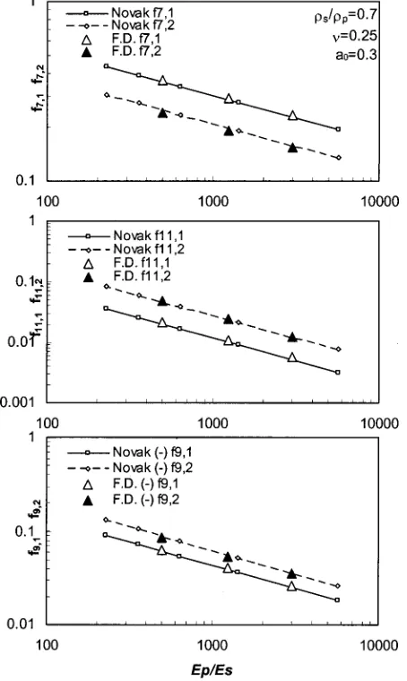
solutions. No material damping was introduced into the model, consistent with Novak’s 1974 solutions. A quiet 共nonreflecting兲 boundary was defined at the model edges, in order to prevent reflection of outward propagating waves back into the model from the boundaries, and to allow the necessary energy radiation. First, a plane strain model of a circular cavity motion was tested, for verification of the FD code’s radiation damping, and the results were compared with Novak’s parameter Su2关see Eq.共2兲兴, which represents the geometric共radiation兲damping. From these calcu-lations, it was found that a distance of approximately 0.7 wave-lengths is required from the cavity to the boundary in order to provide satisfactory representation of the radiation damping. Fig. 3 shows a comparison between Novak’s results, and those ob-tained from the FD computations; the agreement is excellent. Ku-hlemeyer共1979兲showed that Novak’s fi, jparameters plot against Ep/Es as a straight line on a log-log plot, and thus only a few values are needed for evaluating the validity of the proposed method. The FD analyses were performed at three different ratios of Ep/Es共500, 1,250, 3,000兲; the results are presented in Fig. 4. The results were obtained by using two different techniques. In both techniques, the vibration was developed to the steady state condition smoothly, beginning from the static state. In the first technique, a force was applied to the pile head and displacement at the same node was monitored; in the second technique a ve-locity was applied to the pile head and the unbalanced force at the same node was monitored. In the latter case no forces were trans-ferred from the subgrid corresponding to the pile head node, and thus it was necessary to subtract the reaction created in that sub-grid共a velocity boundary and force boundary cannot coexist兲. The results obtained from both techniques were identical. The second technique is suitable for pile group analysis, where all pile heads move rigidly together. Deviation of the FD solutions from No-vak’s solutions are presented in Table 2. NoNo-vak’s values fi jfor the tested Ep/Es were calculated from the power function corre-sponding to Novak’s straight line on the log-log plot. From the comparison presented in Table 2, it can be seen that the greatest deviation relates to the parameter f11.1. Note that the distance between the cavity, which represents the pile, and the quiet boundary, was only 0.4 wavelengths in these calculation runs. The use of this small distance decreased the calculation time signifi-cantly, and thus justified the small deviation it possibly caused.

Uncoupled Model: Pile Group Interaction

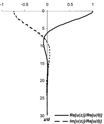
The influence of pile-soil-pile interaction on the behavior of a pile group is well known for static loading. This interaction is quite Fig. 2. Solution shape of Eq.共3兲 for EP/ES⫽1250, ␯⫽0.25, a0

⫽0.3,␳s/␳p⫽0.7共no material damping,␤s⫽0兲

Table 1. Novak’s Stiffness and Damping Parameters

VS/VL EP/ES

Stiffness Parameters Damping Parameters

f11,1 f9,1 f7,1 f11,2 f9,2 f7,2

0.01 5,714.286 0.0032 ⫺0.0181 0.195 0.0076 ⫺0.0262 0.135 0.02 1,428.571 0.009 ⫺0.0362 0.275 0.0215 ⫺0.0529 0.192 0.03 634.9206 0.0166 ⫺0.0543 0.337 0.0395 ⫺0.0793 0.235 0.04 357.1429 0.0256 ⫺0.0724 0.389 0.0608 ⫺0.1057 0.272 0.05 228.5714 0.0358 ⫺0.0905 0.435 0.085 ⫺0.1321 0.304

simple for linear elastic material, and many expressions for evalu-ating it have been suggested共e.g., Poulos 1971b兲. However, this is far from true for a pile group under dynamic loading; dynamic characteristics of pile groups are very complex, strongly fre-quency dependent, and often significantly different from those of a single pile共El-Marsafawi et al. 1992兲. A superposition approach is commonly employed, using complex interaction factors for two piles, in conjunction with known single pile dynamic characteris-tics. Clearly, in using superposition, the interaction between all the piles is approximated. The superposition method is imple-mented through a flexibility approach in conjunction with the dynamic interaction factors for two piles. For a pile group one can write the following relation:

兵Ui其⫽␭s关␣i, j兴兵Pj其 (5)

where Ui⫽head displacement of pile i; ␭s_{⫽single pile dynamic} flexibility; Pj⫽force at the head of pile j; and␣i j⫽complex in-teraction factor between pile i and pile j for a certain vibration mode, defined as the ratio of the dynamic displacement of pile i due to dynamic loading on pile j to the dynamic displacement of pile j. By considering the rigidity of the pile group cap (U⫽Ui ⫽¯⫽Un), one can derive the pile group complex stiffness from Eq. 共5兲, as follows:

Kgroup⫽ 兺j⫽1

n Pj

U ⫽

1 ␭s

兺

i⫽1 n

兺

j⫽1 n

⑀i, j⫽ks

兺

兺

i⫽1 n

⑀i, j (6)

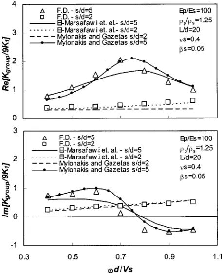
where ks⫽single pile dynamic stiffness; and⑀i, j⫽elements of the inverse of matrix ␣. Design values of interaction factors for dy-namic loading were suggested, for example, by Gazetas et al. 共1991兲and El-Marsafawi et al. 共1992兲. It should be pointed out that, although the superposition method is very convenient for practical usage, a small error in evaluating the interaction factor will result in a much greater error in the group dynamic stiffness. As an example, the group stiffness of a 3⫻3 pile group is com-posed of the summation of 81 values of which 72 are evaluated from design graphs, some by interpolation functions. Winkler models for evaluating the horizontal dynamic pile-soil-pile inter-action in pile groups have also been developed; they all show good agreement with more rigorous solutions based on 3D wave propagation. The simplest Winkler based model is quite new, sug-gested by Mylonakis and Gazetas 共1999兲, yet it is limited by assumptions of linearity for soil and pile materials, and perfect bonding at the soil-pile interface. A more complex model, also based on the Winkler assumption, was proposed by El Nagger and Novak共1996兲. The model accounts for nonlinear behavior of the soil adjacent to the pile and gapping at the soil-pile interface. Although the computational effort is quite small, a computer code designed for that particular model is required. None of the Win-kler model approaches used up to the present have taken account of the disturbance caused by a pile to the waves propagating through the soil medium. When the pile spacing is small, this effect may be of considerable significance. Even the more rigor-ous existing solutions relate the forces to the average displace-ment of the soil-pile interaction segdisplace-ment. Rajapakse and Shah 共1989兲reviewed continuum models for elastic soil pile systems and referred to the averaging procedure as problematic for dy-namic problems. They claimed that with increasing frequency models based on the cross sectional average of the displacement fail to provide an accurate solution. To verify the reliability of the proposed method for the pile-soil-pile interaction, two simple in-teraction problems were considered—two fixed-head piles, and a 3⫻3 pile group. The solutions obtained from the FD analyses were compared with El-Marsafawi et al.’s 共1992兲 solutions, which were based on a 3D boundary integral formulation, and with Mylonakis and Gazetas’共1999兲solutions based on a Winkler model 共propagation of waves in a horizontal manner only兲 in conjunction with superposition. For the case of interaction of two piles, the solutions were obtained for the case in which the hori-zontal translation of the pile head was in the direction of the line connecting the two pile centers. These solutions are presented as an interaction factor between the two piles in Fig. 5. The solution for the case of the 3⫻3 pile group is presented 共Fig. 6兲 as a normalized dynamic stiffness defined as the dynamic stiffness of the pile group divided by the dynamic stiffness of a single pile multiplied by the number of piles in the group. In order to evalu-ate both the two-pile interaction factor and the normalized pile group stiffness, the dynamic stiffness of a single pile must be Fig. 4. Comparison between finite difference solutions and Novak’s

solutions

Table 2. Deviation from Novak’s Solution

EP/ES

Stiffness Parameters Damping Parameters

f11,1 f9,1 f7,1 f11,2 f9,2 f7,2

500 9.66% 5.08% 2.44% 1.87% ⫺3.80% ⫺3.52%

1,250 9.52% 5.28% 2.41% 1.74% ⫺3.41% ⫺3.31%

known. This was found by calculating, with the FD code, the dynamic stiffness of each frequency, in the same manner that was employed in the single-pile dynamic analysis. For the two-pile interaction, excellent agreement between the El-Marsafawi et al. 共1992兲solution and the FD solution exists for a normalized spac-ing (s/d) of 5. However, less good agreement exists for normal-ized spacing of 2, although the Mylonakis and Gazetas Winkler based model shows good agreement with the El-Marasafwi et al. solution. It may be seen that this deviation increases with fre-quency, implying that it is connected to the wave propagation factor. As mentioned previously, both the Winkler based model and the 3D solutions do not comprehensively account for the pile interference to wave propagation, and it is possible that the results from the present calculations take account of this interference. For the 3⫻3 pile group, general agreement exists for all the parameters; interaction of nine piles is quite complex and thus it is difficult to pinpoint the source of the observed deviations.

Uncoupled Model: Single-Pile Seismic Response

Using a Winkler based model for earthquake analysis requires an evaluation of shear wave propagation through the soil layers. Since the plane strain problems are uncoupled共disconnected兲the vertical propagation of shear waves must be modeled separately and applied indirectly to the plane strain problems. This may be done by applying to each grid point, at each time step, an addi-tional force which corresponds to the horizontal acceleration in the free field at the same depth and time. For viscoelastic material this procedure is completely legitimate; it is equivalent to super-position of forces. For nonlinear materials, it is considered to be a reasonable approximation, due to the difference in the polarity of

the S waves in the free field共␶xzand␶y z兲and the␶xystress waves and P waves that would emanate from the pile 共Wang et al. 1998兲; where x is the horizontal direction of pile displacement and z is vertical. Since this formulation decouples the vertical shear propagation from the soil-pile interaction, the free field ac-celeration history may be calculated from an additional one-dimensional analysis within the FD code or an external program such as SHAKE 共Idriss and Sun 1991兲. In this verification prob-lem, the one-dimensional vertical shear propagation was modeled by an additional subgrid which represents the site. A subroutine, which monitors the velocities and acceleration of each grid point in the free field subgrid and inserts them in tables, was written. In every time step an acceleration value for each plane strain prob-lem was interpolated from these tables, according to depth. The acceleration value was then multiplied for each internal共not on a boundary兲grid point by its mass and was applied to it. For the plane strain boundary grid points, a force⌬F defined by Eq.共7兲 was added to the initial K0 static forces in order to maintain nonreflecting boundaries

⌬F⫽maf f⫹C共vf f⫺v兲s (7) where m⫽grid point mass; af f andvf f⫽acceleration and veloc-ity, respectively, of the free field at the same depth;v⫽grid point velocity; C⫽coefficient that is related to the S wave and P wave velocities 共depending on the direction of the applied forces兲; and s⫽boundary length, which is related to the grid point. This for-mulation is very similar to that used in FLAC for free field bound-aries, based on the viscous boundary developed by Lysmer and Kuhlemeyer共1969兲, yet the one implemented in FLAC cannot be used for this formulation. It should be noted that in case a mate-rial damping is defined externally共not within the constitutive re-lation兲it should be activated only on strain rates, i.e., when using Rayleigh damping as in FLAC, the mass proportional damping coefficient should be set to zero. If a mass proportional damping Fig. 6. Normalized lateral dynamic stiffness of 3⫻3 pile group

is defined, the free field vibration modes will be overdamped, since damping is applied both to the free field subgrid, and also to the plane strain system masses.

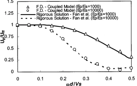
For the verification problem, a fixed-head pile embedded in a homogeneous, viscoelastic soil layer was considered. The base of the soil layer was excited by a harmonic shear wave. In order to represent a homogeneous half space, the shear wave was applied to a quiet boundary. After reaching a steady state motion, the amplitudes of the horizontal oscillation of the pile cap Up and free field surface Uf f were extracted. The FD analyses were per-formed at two different ratios of Ep/Es 共1,000, 10,000兲 for a complete range of frequencies. The results were compared with the rigorous solution of Fan et al.共1991兲based on the boundary integral based formulation developed by Kaynia and Kausel 共1982兲. The results are presented in Fig. 7 as a ratio between the pile cap oscillation amplitude and the free field surface oscillation amplitude.

Good agreement is observed between the results. However, it can be seen that better agreement exists for the higher ratio of Ep/Es. This is consistent with Nogami and Novak’s共1980兲 con-clusion that a soil medium can be treated more favorably as a Winkler based model for stiffer piles.

Limitations of Uncoupled Model

The uncoupled model is based on Winkler’s approach. It may be classified as a first order, dynamic, subgrade model, according to Nogami et al.’s共1992兲definition. Being a first order model, it is bounded by the first order model limitations. It encounters diffi-culties in modeling frequencies lower than the fundamental fre-quency of the soil medium. For machine foundations, this limita-tion is almost irrelevant since the frequencies involved in such cases are usually considerably higher than the fundamental fre-quency of the soil. Also, for earthquakes, most of the soil-pile interaction is noticeable for frequencies around the structure-foundation resonance, which are usually higher than the funda-mental natural frequency of the ground. For floating piles, the first order model is quite accurate. Usually, in order to overcome this limitation of the first order dynamic model, it is modified by using a static stiffness for frequencies lower than the natural one, and ignoring the radiation damping 共Nogami et al. 1992兲. A similar procedure may be invoked in the present procedure for lateral loading of piles, by using a fixed boundary instead of a quiet boundary, so that no energy is absorbed by the boundaries. One

must, of course, be careful in using this procedure, since the lo-cation of the boundaries is crucial in determining the static stiff-ness in a plane strain problem. Baguelin et al.共1977兲have con-ducted a theoretical study of the static lateral reaction mechanism of piles using plane strain analysis. Their recommendation for the boundary locations may be adopted, but it should be appreciated that unnecessary amplification is possible in dynamic analyses. However, it is possible to overcome all limitation of first order models by coupling the plane strain problems. This modification is presented in the following section.

Coupled Model

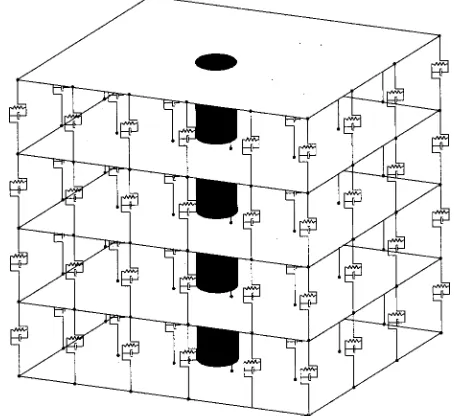
A coupling of the plane strain problems is feasible by connecting shear springs and dashpots between every plane strain problem grid point and the upper/lower plane strain problem grid point. A schematic representation of coupling the plane strain problems with springs and dashpots is presented in Fig. 8. This coupling may or may not actually be a part of the constitutive model for the soil. The use of springs and dashpots for homogenous elastic material is equivalent to the use of terms obtained from the equa-tion of moequa-tion for a continuous body

␳⳵ 2_u

j ⳵t2 ⫽␳gj⫹

⳵␴i j ⳵xi

(8)

where uj⫽displacement vector; ␳⫽density; t⫽time; gj ⫽gravitation vector; and␴i j⫽stress tensor. By restricting the mo-tion to the horizontal planes, only the variamo-tion of displacement with depth needs to be considered for the coupling. An additional force vector should be applied to the concentrated masses located at the corners of the FD zones共grid points兲

Fj⫽ M

␳ ⳵␴z j

⳵z ⫽ M

␳

⳵共2G⑀z j⫹2G␩⑀˙z j兲 ⳵z

⫽M_␳ G

冉

j ⳵z2 ⫹␴

⳵2_u˙ j

⳵z2

冊

where Fj⫽additional force vector applied to the mass; M ⫽mass value of the grid point; G⫽shear modulus; ␩ Fig. 7. Kinematic seismic response of single fixed-head pile in

ho-mogeneous soil layer共␳s/␳p⫽0.7,␤s⫽0.05,␯⫽0.4兲

⫽parameter related to the viscous damping and frequency; z ⫽vertical axis; and j takes the index of the horizontal axes. Re-writing Eq.共9兲using finite difference approximations of the de-rivatives results in the same expression that is obtained by using springs and dashpots with values of K⫽G/l and C⫽␩G/l, re-spectively, and correcting from stress to force by applying an ‘‘area factor’’ of M /␳d to the applied grid point force共l is the distance between the layers connected by the springs and dash-pots and d is the thickness of the horizontal layer that the plane strain problem represents兲. One can regard this model as a true 3D model where all the grid points are constrained共fixed兲in the vertical direction. Wu and Finn共1997a, b兲presented a quasi-3D finite element model, where the grid point motion was fixed both in the vertical direction and in the direction perpendicular to the pile motion. However, instead of using a nonreflecting 共quiet兲 boundary they applied dashpots to the pile shaft to model the radiation damping. Although the form of these dashpot coeffi-cients was based on a simple, one-dimensional ‘‘cone’’ model 共Gazetas et al. 1993兲, they were calibrated by curve-fitting results from rigorous, finite element analyses, where no limitation was made on grid point movements. Reduction of degrees of freedom in an implicit integral method is more computationally effective than it is in explicit integral methods where no factorization of matrices is necessary. Consequently, Wu and Finn’s approach may be more justified for implicit schemes than for explicit schemes. Several problems with different pile configurations and load-ing conditions are presented in the followload-ing sections for verifi-cation of the proposed coupled model.

Coupled Model: Static Lateral Loading

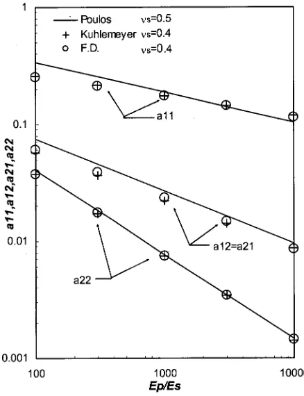
One of the disadvantages of the uncoupled model is that it cannot model a case of static loading, since there is no solution for plane strain loading in an infinite homogeneous material关i.e., in a nu-merical analysis the solution is boundary dependent; Baguelin et al. 共1977兲studied the necessary distance of a fixed boundary for simulation of static stiffness兴. However, with the coupled model, such a static case is solvable, and was therefore chosen as one of the verification problems. The analysis was conducted for a homogeneous soil modeled as a linear elastic material. The single pile was pinned at its base to a solid rock. However, this end condition had no influence on the results and the solution may be regarded as that for a floating pile, since the pile length was significantly longer than its effective length. Since the calculation involved a linear elastic material, it was more convenient to de-fine behavior of the coupling springs共Voigt elements兲separately from the constitutive relation of the soil. In order to assess accu-racy, a comparison to Poulos’s共1971a兲results共based on coupling Mindlin’s solution for a concentrated horizontal load with the pile flexure equation兲, and to Kuhlemeyer’s共1979兲3D finite element results, was conducted. The solutions are presented in Fig. 9 in terms of Kuhlemeyer’s formulations

U⫽a11 P Esr0⫹

a12 M Esr0

2

(10)

⌽⫽a21 P Esr0

2⫹a22 M Esr0

3

where ai j are parameters that are functions of the Poisson ratio and (Ep/Es) ratio. Poulos presented his solutions in the form

U⫽IUS P EsL⫹

IUR M

EsL2 ₍₁₁₎

⌽⫽I_␪S P EsL2⫹

I_␪R M EsL3

where IUS, IUR, I␪S, and I␪R are functions of L/r0 and the pile flexibility factor KR⫽EpIp/EsL4. Presenting Poulos’s results ac-cording to Kuhlemeyer’s formulation leads to the identity

a11⫽ IUS L/r0

; a12⫽a21⫽ IUR 共L/r0兲2

; a22⫽ I_␪R 共L/r0兲3

(12)

Excellent agreement exists between the coupled model results and Kuhlemeyer’s results, the largest deviation being smaller than 5%. It should be noted that Kuhlemeyer’s results are rigorous, obtained by a real, 3D analysis where every grid point is free to move in all directions, and not only horizontally. This small de-viation might suggest that the restraint of movement in the verti-cal direction causes the soil-pile system to stiffen only slightly. The cause for deviation of Poulos’s results was explained by Kuh-lemeyer 共1979兲, and will not be discussed here. However it should be noted that some of Poulos’s results are considered to be in error due to numerical discretization. Comparisons with other static stiffness values obtained by finite element methods and boundary integral formulation 共Randolph 1981; Dobry et al. 1982; Kaynia and Kausel 1991兲were also conducted. The agree-ment with Randolph’s solution is more or less as with Kuh-lemeyer’s solution. The deviations from Dobry et al.’s results 共based on a finite element code developed by Blaney et al. 1976兲 are up to 20%. It should be noted that a similar difference exists between the Dobry et al. and Kuhlemeyer solutions, probably due to different discretization and boundary conditions. The present static value of stiffness is about 10% higher than that reported by Kaynia and Kausel共1991兲.

Coupled Model: Dynamic Lateral Loading

In order to verify the behavior of the coupled model under dy-namic excitation, a simple problem of dydy-namic lateral loading was considered, and the results were compared with a continuum solution based on the work of Tajimi 共1969兲. As for the case of static lateral loading, the analysis was conducted for a homoge-neous soil, modeled as a viscoelastic material. The comparison was made for the lateral translation stiffness, as presented in Fig. 10 for the case of L/r0⫽38.5, ␳s/␳p⫽0.625, ␯⫽0.4, VS/VL ⫽0.044 共or Ep/Es⫽295.159兲with material damping ␤s⫽0 and 5%. It can be seen from Fig. 10 that both the real and imaginary parts of the complex stiffness are in excellent agreement with the solution based on Tajimi’s work. It is seen from Fig. 10 that the coupled model captures the phenomenon of decreased stiffness around the natural fundamental frequencies and the overall shape. The radiation damping cutoff frequency is also well modeled. Since Tajimi’s共1969兲formulation imperfectly captures the mate-rial damping behavior共it is taken into account only for the shear waves traveling along the depth and not for shear waves traveling horizontally兲, it was necessary to modify his formulation for more accurate consideration of material damping. A frequency indepen-dent viscosity was introduced into the equations of the elastic continuum by complementing Lame´’s constants with their imagi-nary共out-of-phase兲components.

Coupled Model: Single-Pile Seismic Response

Unlike Winkler based models, the coupled model inherently cap-tures the development of shear stresses 共␶xz and ␶y z兲; thus no

separate modeling of free fields is required for superposition of forces. However, in order to allow dissipation of pile vibration energy 共radiation damping兲 to the infinite soil, nonreflecting boundaries are used together with the free field calculation. These boundaries are not mandatory; an alternative approach is to locate the plane strain problem boundaries at a sufficient distance from the pile. In this case, waves emitted from the pile will dissipate due to material damping. For soils with low material damping the latter approach is impractical, since a large number of soil ele-ments is required. Again, the formulation of the nonreflecting boundary共free field boundary兲is similar to that used in FLAC for plane strain problems, based on the viscous boundary developed by Lysmer and Kuhlemeyer 共1969兲. FLAC’s built-in free field boundary cannot be applied to the proposed model since its for-mulation is limited to a single plane strain problem where the grid represents a vertical plane. Fig. 11 demonstrates the mechanism of the free field boundary. It comprises a column of concentrated masses connected by springs共detail A兲with each mass connected to a plane strain system through a viscous elements 共detail B兲. A one-dimensional free field is modeled by discrete masses con-nected by the coupling springs simultaneously with analysis of the plane strain problems. The free field motion may also be modeled by a plane strain problem共a vertical bar兲with a suitable constitutive law, but using the same springs for the free field calculation as for the coupling is numerically more accurate. At each time step an additional force is applied to the boundaries via the viscous element, according to the expression

⌬F⫽C共vf f⫺v兲s (13) where the terms are as defined in Eq.共7兲. It can be noted from Eq. 共13兲 that if the main grid motion is identical to the free field motion 共i.e.,v⫽v_{f f}兲the dashpots共illustrated in Fig. 11兲are not exercised. However, if the main grid motion differs from that of the free field, then the dashpots act to absorb energy. Evaluation of the free field motion can also be conducted with an external program such as SHAKE. However, since the vertical propagation of the waves would be different, even slightly, from those of the main grid, the dashpots would be unnecessarily exercised and might cause unreasonable results. The verification problem con-Fig. 10. Comparison of dynamic lateral stiffness computed by finite

difference to values based on Tajimi

sidered was identical to that of the uncoupled model. Again, re-sults were compared with the rigorous solution of Fan et al. 共1991兲, and are presented in Fig. 12. Excellent agreement is noted between the results.

Scope of Method

The presented technique and models may be used for solving a vast variety of soil-pile interaction problems; they are not re-stricted to linear elastic materials nor to homogeneous soil layers. For the uncoupled model, any desired constitutive law may be invoked by using either one of the FD code’s library of constitu-tive relations, or by introducing a new relation through an internal subroutine. However, for the coupled model, an additional sub-routine must be written in order to incorporate a constitutive law, since the coupling option is a modification of the code. Soil-pile gapping may be considered by inserting an interface at the cavity boundary. Moreover, in the case of a soil in which the permeabil-ity is significantly higher in the horizontal direction, a fully coupled analysis of pile-soil-groundwater interaction may be solved, according to the assumption that the water pressure will dissipate only in the horizontal direction. For soil with permeabil-ity equal in all directions, Nogami and Kazama 共1991兲showed that analytical expressions for pile lateral stiffness in a fluid satu-rated porous medium using cylindrical plane strain conditions yield results with accuracy very similar to those obtained for single-phase solids, which are well accepted. The method may also be used to solve loading in two directions, by assuming that the pile is linear elastic and analyzing two unsupported beams which represent the principal axes of the pile.

Conclusions

A general approach, based on the commercial 2D finite difference code FLAC, for evaluating the soil-pile interaction of single piles and pile groups under static, seismic, and lateral dynamic loading was presented. Two models were derived using this approach. Good agreement, for both models, was obtained with true 3D models and Winkler models for simple verification problems.

The uncoupled model has an advantage over the true 3D model, since discretization along the vertical axis is determined by the soil-pile characteristics and not only by the soil; thus fewer zones need to be defined. Its main advantage over other Winkler

type models is that the behavior of the soil may be defined by a constitutive relation, and not just by spring coefficients or empiri-cal p-y curves. The coupled model may be considered an expan-sion of the uncoupled model, overcoming most of its limitations. A major advantage of the technique presented is that it can easily be implemented by any practicing engineer, with minor knowledge of numerical methods, using a computer code that is relatively inexpensive compared with true 3D programs.

Acknowledgment

The research described in this paper is supported by the Israel Ministry of Housing and Construction, through the National Building Research Station at the Technion.

Notation

The following symbols are used in this paper: a0 ⫽ dimensionless frequency;

af f, vf f ⫽ free field acceleration and velocity; Ep ⫽ Young’s modulus of pile;

Es ⫽ Young’s modulus of soil; fi, j ⫽ stiffness parameters of pile;

Ip ⫽ inertia moment of pile cross section; IUS, IUR, I␪S, I␪R

⫽ Poulos’s parameters; ks _{⫽ single-pile stiffness;} kus ⫽ horizontal soil stiffness;

L ⫽ length of pile;

P, M ⫽ horizontal force and moment applied to pile’s head;

r0,d ⫽ radius and diameter of pile; Su1, Su2 ⫽ soil stiffness parameters;

s/d ⫽ normalized distance between piles; U ⫽ horizontal translation at head of pile;

u ⫽ horizontal displacement along pile; VL ⫽ longitudinal wave velocity of pile; V_P, V_S ⫽ P wave and S wave velocities of soil;

␣i, j ⫽ interaction factors;

␤s ⫽ material damping of soil;

⑀i, j ⫽ values of inverse matrix of interaction factors;

␭s _{⫽ single-pile flexibility;}

␮ ⫽ mass of pile per unit length; ␯ ⫽ Poisson’s ratio;

␳p ⫽ density of pile;

␳s ⫽ density of soil;

⌽ ⫽ rotation at head of pile; and ␻ ⫽ circular frequency.

References

Baguelin, F., Frank, R., and Said, Y. H. 共1977兲. ‘‘Theoretical study of lateral reaction mechanism of piles.’’ Geotechnique, 27共3兲, 405– 434. Blaney, G. W., Kausel, E., and Roesset, J. M.共1976兲. ‘‘Dynamic stiffness of piles.’’ Proc., 2nd Int. Conf. on Numerical Methods in Geomechan-ics, ASCE, Blacksburg, Va., Vol. II, 1001–1012.

Dobry, R., Vicente, E., O’Rouke, M., and Roesset, J.共1982兲. ‘‘Horizontal stiffness and damping of single piles.’’ J. Geotech. Eng., 108共3兲, 439– 459.

El-Marsafawi, H., Kaynia, A., and Novak, M.共1992兲. ‘‘The superposition approach to pile group dynamics.’’ Geotechnical engineering divi-Fig. 12. Kinematic seismic response of single, fixed-head pile in

sion special publication No. 34, ASCE, New York, 114 –135. El Nagger, M. H., and Novak, M.共1996兲. ‘‘Nonlinear analysis for

dy-namic lateral pile response.’’ Soil Dyn. Earthquake Eng., 15, 233– 244.

Fan, K., Gazetas, G., Kaynia, A., Kausel, E., and Ahmad, S. 共1991兲. ‘‘Kinematic seismic response of single piles and pile groups.’’ J. Geo-tech. Eng., 117共12兲, 1860–1879.

Gazetas, G., Fan, K., and Kaynia, A.共1993兲. ‘‘Dynamic response of pile groups with different configurations.’’ Soil Dyn. Earthquake Eng., 12共4兲, 239–257.

Gazetas, G., Fan, K., Kaynia, A., and Kausel, E.共1991兲. ‘‘Dynamic in-teraction factors for floating pile groups.’’ J. Geotech. Eng., 117共10兲, 1531–1548.

Idriss, I. M., and Sun, J.共1991兲. User’s Manual for SHAKE91, Center for Geotechnical Modeling, Dept. of Civil and Environmental Engineer-ing, Univ. of California, Davis, Calif.

Itasca.共1999兲. FLAC—Theory and background, Version 3.4, Itasca Con-sulting Group, Inc., Minneapolis.

Kagawa, T.共1983兲. NONSPS: User manual, McClelland Engineers, Inc., Houston.

Kaynia, A. M., and Kausel, E. 共1982兲. ‘‘Dynamic stiffness and seismic response of pile groups.’’ Research Rep., Dept. of Civil Engineering, Massachusetts Institute of Technology, Cambridge, Mass.

Kaynia, A. M., and Kausel, E. 共1991兲. ‘‘Dynamics of piles and pile groups in layered soil media.’’ Soil Dyn. Earthquake Eng., 10共8兲, 386 – 401.

Kuhlemeyer, R. 共1979兲. ‘‘Static and dynamic laterally loaded floating piles.’’ J. Geotech. Eng., 105共2兲, 289–304.

Lysmer, J., and Kuhlemeyer, R. L.共1969兲. ‘‘Finite dynamic model for infinite media.’’ J. Eng. Mech. Div., 95共EM4兲, 859– 877.

Mamoon, S. M., Banerjee, P. K., and Ahmad, S. 共1988兲. ‘‘Seismic re-sponse of pile foundations.’’ Technical Rep. No. NCEER-88-003, Dept. of Civil Engineering, State Univ. of New York, Buffalo, N.Y. Mylonakis, G., and Gazetas, G.共1999兲. ‘‘Lateral vibration and internal

forces of grouped piles in layered soil.’’ J. Geotech. Geoenviron. Eng., 125共1兲, 16 –25.

Nogami, T., and Kazama, M.共1991兲. ‘‘Effects of offshore environment on dynamic response of pile foundation.’’ Final Rep. to Mineral Man-agement Service, Scripps Institution of Oceanography, University of California at San Diego, La Jolla, Calif.

Nogami, T., and Novak, M.共1980兲. ‘‘Coefficients of soil reaction to pile vibration.’’ J. Geotech. Eng., 106共5兲, 565–570.

Nogami, T., Zhu, J. X., and Ito, T.共1992兲. ‘‘First and second order dy-namic subgrade models for soil-pile interaction analysis.’’ Geotechni-cal Engineering Division, Special Publication No. 34, ASCE, New York, 187–206.

Novak, M.共1974兲. ‘‘Dynamic stiffness and damping of piles.’’ Can. Geo-tech. J., 11共4兲, 574 –598.

Novak, M., and Aboul-Ella, F.共1978兲. ‘‘Impedance functions of piles in layered media.’’ J. Geotech. Eng., 104共3兲, 643– 661.

Novak, M., and El-Sharnouby, B.共1983兲. ‘‘Stiffness constants of single piles.’’ J. Geotech. Eng., 109共7兲, 961–974.

Novak, M., Nogami, T., and Aboul-Ella, F.共1978兲. ‘‘Dynamic soil reac-tions for plane strain case.’’ J. Geotech. Eng., 104共4兲, 953–959. Novak, M., Sheta, M., El-Hifnawy, L., El-Marsafawi, H., and Ramadan,

O.共1990兲DYNA3: A computer program for calculation of foundation response to dynamic loads, Geotechnical Research Center, Univ. of Western Ontario, London, Ont., Canada.

Poulos, H.共1971a兲. ‘‘Behavior of laterally loaded piles: I—Single piles.’’ J. Soil Mech. Found. Div., 97共5兲, 711–731.

Poulos, H.共1971b兲. ‘‘Behavior of laterally loaded piles: II—Pile groups.’’ J. Soil. Mech. Found. Div., 97共5兲, 733–751.

Rajapakse, R. K. N. D., and Shah, A. H.共1989兲. ‘‘Impedance curves for an elastic pile.’’ Soil Dyn. Earthquake Eng., 8共3兲, 145–152. Randolph, M. F.共1981兲. ‘‘The response of flexible piles to lateral

load-ing.’’ Geotechnique, 31共2兲, 247–259.

Tajimi, H. 共1969兲. ‘‘Dynamic analysis of a structure embedded in an elastic stratum.’’ Proc., 4th World Conf. on Earthquake Engineering, Chile Association on Seismology and Earthquake Engineering, San-tiago, Chile, Vol. 3, 53– 69.

Wang, S., Kutter, B. L., Chacko, M. J., Wilson, D. W., Boulanger, R. W., and Abghari, A.共1998兲. ‘‘Nonlinear seismic soil-pile structure inter-action.’’ Earthquake Spectra, 14共2兲, 377–396.

Wu, G., and Finn, W.共1997a兲. ‘‘Dynamic elastic analysis of pile founda-tions using finite element method in the frequency domain.’’ Can. Geotech. J., 34共1兲, 34 – 43.