Distance-Based Classification with Lipschitz Functions

Distance-Based Classification with Lipschitz Functions

Ulrike von Luxburg [email protected]

Olivier Bousquet [email protected]

Max Planck Institute for Biological Cybernetics Spemannstrasse 38

72076 T¨ubingen, Germany

Editors: Kristin Bennett and Nicol `o Cesa-Bianchi

Abstract

The goal of this article is to develop a framework for large margin classification in metric spaces. We want to find a generalization of linear decision functions for metric spaces and define a corre-sponding notion of margin such that the decision function separates the training points with a large margin. It will turn out that using Lipschitz functions as decision functions, the inverse of the Lip-schitz constant can be interpreted as the size of a margin. In order to construct a clean mathematical setup we isometrically embed the given metric space into a Banach space and the space of Lipschitz functions into its dual space. To analyze the resulting algorithm, we prove several representer theo-rems. They state that there always exist solutions of the Lipschitz classifier which can be expressed in terms of distance functions to training points. We provide generalization bounds for Lipschitz classifiers in terms of the Rademacher complexities of some Lipschitz function classes. The gen-erality of our approach can be seen from the fact that several well-known algorithms are special cases of the Lipschitz classifier, among them the support vector machine, the linear programming machine, and the 1-nearest neighbor classifier.

1. Introduction

Support vector machines (SVMs) construct linear decision boundaries in Hilbert spaces such that the training points are separated with a large margin. The goal of this article is to extend this approach from Hilbert spaces to metric spaces: we want to find a generalization of linear decision functions for metric spaces and define a corresponding notion of margin such that the decision function separates the training points with a large margin. The reason why we are interested in metric spaces is that in many applications it is easier or more natural to construct distance functions between objects in the data space than positive definite kernel functions as they are used for support vector machines. Examples for this situation are the edit distance used to compare strings or graphs and the earth mover’s distance on images.

SVMs can be seen from two different points of view. In the regularization interpretation, for a given positive definite kernel k, the SVM chooses a decision function of the form f(x) =

∑iαik(xi,x) +b which has a low empirical error Remp and is as smooth as possible. According to

the large margin point of view, SVMs construct a linear decision boundary in a Hilbert space

H

such that the training points are separated with a large margin and the sum of the margin errors is

small. Both viewpoints can be connected by embedding the sample space

X

into the reproducing

norm of a linear operator), and the empirical error corresponds to the margin error (cf. Sections 4.3 and 7 of Sch ¨olkopf and Smola, 2002). The benefits of these two dual viewpoints are that the reg-ularization framework gives some intuition about the geometrical meaning of the norm on

H

, and the large margin framework leads to statistical learning theory bounds on the generalization error of the classifier.

Now consider the situation where the sample space is a metric space(

X

,d). From the regular-ization point of view, a convenient set of functions on a metric space is the set of Lipschitz functions, as functions with a small Lipschitz constant have low variation. Thus it seems desirable to separate the different classes by a decision function which has a small Lipschitz constant. In this article we want to construct the dual point of view to this approach. To this end, we embed the metric space

(

X

,d)in a Banach space

B

and the space of Lipschitz functions into its dual space

B

0. Remarkably, both embeddings can be realized as isometries simultaneously. By this construction, each x_∈

X

will correspond to some mx∈

B

and each Lipschitz function f on

X

to some functional Tf ∈

B

0 such

that f(x) =Tfmxand the Lipschitz constant L(f)is equal to the operator normkTfk. In the Banach

space

B

we can then construct a large margin classifier such that the size of the margin will be given by the inverse of the operator norm of the decision functional. The basic algorithm implementing this approach is

minimize Remp(f) +λL(f)

in regularization language and

minimize L(f) +C

∑

_iξisubject to yif(xi)≥1−ξi,ξi≥0

in large margin language. In both cases, L(f) denotes the Lipschitz constant of the function f , and the minimum is taken over a subset of Lipschitz functions on

X

. To apply this algorithm in practice, the choice of this subset will be important. We will see that by choosing different sub-sets we can recover the SVM (in cases where the metric on

X

is induced by a kernel), the linear programming machine (cf. Graepel et al., 1999), and even the 1-nearest neighbor classifier. In par-ticular this shows that all these algorithms are large margin algorithms. So the Lipschitz framework can help to analyze a wide range of algorithms which do not seem to be connected at the first glance.

This paper is organized as follows: in Section 2 we provide the necessary functional analytic background for the Lipschitz algorithm, which is then derived in Section 3. We investigate rep-resenter theorems for this algorithm in Section 4. It will turn out that the algorithm always has a solution which can be expressed by distance functions to training points. In Section 5 we compute error bounds for the Lipschitz classifier in terms of Rademacher complexities. In particular, this gives valuable information about how fast the algorithm converges for different choices of subsets of Lipschitz functions. The geometrical interpretation for choosing different subsets of Lipschitz functions is further discussed in Section 6.

2. Lipschitz Function Spaces

In this section we introduce several Lipschitz function spaces and their properties. For a compre-hensive overview we refer to Weaver (1999).

d(y,z)_≤d(x,z). A function f :

X

→ on a metric space(

X

,d)is called a Lipschitz function if there exists a constant L such that_|f(x)₋f(y)_{| ≤}Ld(x,y)for all x,y_∈

X

. The smallest constant L such that this inequality holds is called the Lipschitz constant of f , denoted by L(f). For convenience, we recall some standard facts about Lipschitz functions:

Lemma 1 (Lipschitz functions) Let(

X

,d)be a metric space, f,g :

X

_→ Lipschitz functions and a_∈ . Then L(f+g)_≤L(f) +L(g), L(a f)_{≤ |}a_|L(f)and L(min(f,g))_≤max_{L(f),L(g)_}, where

min(f,g)denotes the pointwise minimum of the functions f and g. Moreover, let f :=limn→∞fnthe pointwise limit of Lipschitz functions fnwith L(fn)≤c for all n∈ . Then f is a Lipschitz function with L(f)_≤c.

For a metric space(

X

,d)consider the set

Lip(

X

):=_{f :

X

_→ ; f is a bounded Lipschitz function_}.

It forms a vector space, and the Lipschitz constant L(f) is a seminorm on this space. To define a convenient norm on this space we restrict ourselves to bounded metric spaces. These are spaces which have a finite diameter diam(

X

):=sup_x,y∈Xd(x,y). For the learning framework this is not a big drawback as the training and test data can always be assumed to come from a bounded region

of the underlying space. For a bounded metric space

X

we choose the norm

kf_kL:=max

L(f), kfk∞

diam(

X

)

as our default norm on the space Lip(

X

). It is easy to see that this indeed is a norm. Note that in the mathematical literature, Lip(

X

)is usually endowed with the slightly different norm_kf_k:=

max_{L(f),_kf_k∞}. But we will see that the norm_k·kLfits very naturally in our classification setting,

as already can be seen by the following intuitive argument. Functions that are used as classifiers are supposed to take positive and negative values on the respective classes and satisfy

kf_k∞=sup

x |

f(x)_{| ≤}sup

x,y |

f(x)₋f(y)_{| ≤}diam(

X

)L(f), (1)

that is _kf_kL=L(f).Hence, the L-norm of a classification decision function is determined by the

quantity L(f) we use as regularizer later on. Some more technical reasons for the choice of_{k · k}L

will become clear later.

Another important space of Lipschitz functions is constructed as follows. Let(

X

0,d)be a metric

space with a distinguished “base point” e which is fixed in advance. (

X

0,d,e)is called a pointed

metric space. We define

Lip₀(

X

0):={f ∈Lip(

X

0); f(e) =0}.

On this space, the Lipschitz constant L(_·) is a norm. However, its disadvantage in the learning framework is the condition f(e) =0, which is an inconvenient a priori restriction on our classifier as e has to be chosen in advance. To overcome this restriction, for a given bounded metric space

(

X

,d) we define a corresponding extended pointed metric space

X

0:=

X

∪ {e} for a new base

element e with the metric

dX0(x,y) = (

d(x,y) for x,y_∈

X

Note that diam(

X

0) =diam(

X

). Then we define the map

ψ: Lip(

X

)_→Lip₀(

X

0), ψ(f)(x) =

(

f(x) if x_∈

X

0 if x=e. (3)

Lemma 2 (Isometry between Lipschitz function spaces) ψis an isometric isomorphism between

Lip(

X

)and Lip₀(

X

0).

Proof Obviously,ψis bijective and linear. Moreover, for f0:=ψ(f)we have

L(f0) = sup

x,y∈X0

|f0(x)−f0(y)| dX0(x,y)

=max{sup

x,y∈X

|f(x)₋f(y)_| d(x,y) ,supx∈X

|f(x)₋f(e)_| dX0(x,e)

}=

= max_{L(f), kfk∞

diam(

X

)}=kfkL.

Hence,ψis an isometry.

In some respects, the space(Lip₀(

X

0),L(·))is more convenient to work with than(Lip(

X

),k · kL). In particular it has some very useful duality properties. Let(

X

0,d,e)be a pointed metric space

with some distinguished base element e. A molecule of

X

0 is a function m :

X

0→ such that its

support (i.e., the set where m has non-zero values) is a finite set and∑x∈X0m(x) =0. For x,y∈

X

0

we define the basic molecules mxy:= x− y. It is easy to see that every molecule m can be written

as a (non unique) finite linear combination of basic molecules. Thus we can define

kmkAE:=inf

(

∑

i

|ai|d(xi,yi); m=

∑

i

aimxiyi

)

which is a norm on the space of molecules. The completion of the space of molecules with respect to_{k · k}AE is called the Arens-Eells space AE(

X

0). Denoting its dual space (i.e., the space of all

continuous linear forms on AE(

X

0)) by AE(

X

0)0 the following theorem holds true (cf. Arens and

Eells, 1956; Weaver, 1999).

Theorem 3 (Isometry between AE(

X

0)0and Lip0(

X

0)) AE(

X

0)0 is isometrically isomorphic to

Lip₀(

X

0).

This means that we can regard a Lipschitz function f on

X

0as a linear functional Tf on the space of

molecules, and the Lipschitz constant L(f)coincides with the operator norm of the corresponding functional Tf. For a molecule m and a Lipschitz function f this duality can be expressed as

hf,m_i=

∑

x∈X0

m(x)f(x). (4)

It can be proved that_kmxykAE=d(x,y)holds for all basic molecules mxy. Hence, it is possible to

embed

X

0isometrically in AE(

X

0)via

The normk · kAEhas a nice geometrical interpretation in terms of the mass transportation prob-lem (cf. Weaver, 1999): some product is manufactured in varying amounts at several factories and

has to be distributed to several shops. The (discrete) transportation problem is to find an optimal way to transport the product from the factories to the shops. The costs of such a transport are defined as∑i jai jdi jwhere ai j denotes the amount of the product transported from factory i to shop j and di j

the distance between them. If fidenotes the amount produced in factory i and sidenotes the amount

needed in shop i, the formal definition of the transportation problem is

min

i,j=1,...,n

∑

ai jdi j subject to ai j≥0,

∑

_j ai j=sj,

∑

_i ai j= fi. (6)

To connect the Arens-Eells space to this problem we identify the locations of the factories and shops with a molecule m. The points x with m(x)>0 represent the factories, the ones with m(x)<0 the shops. It can be proved that_km_kAE equals the minimal transportation costs for molecule m. A

special case is when the given molecule has the form m0=∑mxiyj. In this case, the transportation

problem reduces to the bipartite minimal matching problem: given 2m points(x1, . . . ,xn,y1, . . . ,yn)

in a metric space, we want to match each of the x-points to one of the y-points such that the sum of the distances between the matched pairs is minimal. The formal statement of this problem is

min

π

∑

_i,jd(xi,yπ(i)) (7)

where the minimum is taken over all permutationsπof the set_{1, ...,n_}(cf. Steele, 1997).

In Section 4 we will also need the notion of a vector lattice. A vector lattice is a vector space V with an orderingwhich respects the vector space structure (i.e., for x,y,z_∈V,a>0: xy =_⇒ x+ zy+z and axay) and such that for any two elements f,g_∈V there exists a greatest lower bound

inf(f,g). In particular, the space of Lipschitz functions with the ordering f g _{⇔ ∀}x f(x)_≤g(x)

forms a vector lattice.

3. The Lipschitz Classifier

Let(

X

,d)be a metric space and(xi,yi)i=1,...,n⊂

X

× {±1}some training data. In order to be able

to define hyperplanes, we want to embed(

X

,d)into a vector space, but without loosing or changing the underlying metric structure.

3.1 Embedding and Large Margin in Banach Spaces

Our first step is to embed

X

by the identity mapping into the extended space

X

0as described in (2),

which in turn is embedded into AE(

X

0)via (5). We denote the resulting composite embedding by

Φ:

X

_→AE(

X

0),x7→mx:=mxe.

Secondly, we identify Lip(

X

)with Lip₀(

X

0)according to (3) and then Lip0(

X

0) with AE(

X

0)0

ac-cording to Theorem 3. Together this defines the map

Ψ: Lip(

X

)_→AE(

X

0)0, f7→Tf.

1. Φis an isometric embedding of

X

into AE(

X

0): to every point x∈

X

corresponds a molecule mx∈AE(

X

0)such that d(x,y) =kmx−mykAE for all x,y∈

X

.

2. Lip(

X

) is isometrically isomorphic to AE(

X

0)0: to every Lipschitz function f on

X

corre-sponds an operator Tf on AE(

X

0)such thatkfkL=kTfkand vice versa.

3. It makes no difference whether we evaluate operators on the image of

X

in AE(

X

0)or apply Lipschitz functions on

X

directly: Tfmx= f(x).

4. Scaling a linear operator is the same as scaling the corresponding Lipschitz function: for a_∈ we have aTf =Ta f.

Proof All these properties are direct consequences of the construction and Equation (4).

The message of this lemma is that it makes no difference whether we classify our training data on the space

X

with the decision function sgn f(x)or on AE(

X

0)with the hyperplane sgn(Tfmx).

The advantage of the latter is that constructing a large margin classifier in a Banach space is a well studied problem. In Bennett and Bredensteiner (2000) and Zhou et al. (2002) it has been established that constructing a maximal margin hyperplane between the set X+ of positive and X−of negative training points in a Banach space V is equivalent to finding the distance between the convex hulls of

X+and X−. More precisely, let C+and C−the convex hulls of the sets X+and X−. In the separable case, we define the margin of a separating hyperplane H between C+and C−as the minimal distance between the training points and the hyperplane:

ρ(H):= inf

i=1,...,nd(xi,H).

The margin of the maximal margin hyperplane coincides with half the distance between the convex hulls of the positive and negative training points. Hence, determining the maximum margin hyperplane can be understood as solving the optimization problem

inf

p+_∈C+_,p−_∈C−kp +

−p−_k.

By duality arguments (cf. Bennett and Bredensteiner, 2000) it can be seen that its solution coincides with the solution of

sup

T∈V0

inf

p+∈C+,p−∈C−hT,p

+_−p−_i/kTk.

This can be equivalently rewritten as the optimization problem

inf

T_∈V0_,b∈ kTksubject to yi(hT,xii+b)≥1 ∀i=1, ...,n. (8)

A solution of this problem is called a large margin classifier. The decision function has the form

3.2 Derivation of the Algorithm

Now we can apply this construction to our situation. We embed

X

isometrically into the Banach

space AE(

X

0)and use the above reasoning to construct a large margin classifier. As the dual space

of AE(

X

0)is Lip0(

X

0)andhf,mxi=f(x), the optimization problem (8) in our case is

inf

f0∈Lip0(X0),b∈

L(f0)subject to yi(f0(xi) +b)≥1 ∀i=1, ...,n.

By the isometry stated in Theorem 3, this is equivalent to the problem

inf

f_∈Lip(X),b_∈ kfkLsubject to yi(f(xi) +b)≥1 ∀i=1, ...,n.

Next we want to show that the solution of this optimization problem does not depend on the variable b. To this end, we first set g := f+b_∈Lip(

X

)to obtain

inf

g∈Lip(X),b∈ kg−bkLsubject to yig(xi)≥1 ∀i=1, ...,n. Then we observe that

kg₋b_kL=max{L(g−b),k

g₋b_k∞

diam(

X

)}=max{L(g),

kg₋b_k∞

diam(

X

)} ≥L(g) =max{L(g),

kg_k∞

diam(

X

)}.

Here the last step is true because of the fact that g takes positive and negative values and thus

kg_k∞/diam(

X

)_≤L(g)as we explained in Equation (1) of Section 2. Hence, under the constraints

yig(xi)≥1 we have infbkg−bkL=L(g), and we can rewrite our optimization problem in the final

form

inf

f∈Lip(X)L(f)subject to yif(xi)≥1,i=1, . . . ,n. (∗)

We call a solution of this problem a (hard margin) Lipschitz classifier. So we have proved:

Theorem 5 (Lipschitz classifier) Let(

X

,d)be a bounded metric space,(xi,yi)i=1,...,n⊂

X

×{±1} some training data containing points of both classes. Then a solution f of (_∗) is a large margin

classifier, and its margin is given by 1/L(f).

One nice aspect about the above construction is that the margin constructed in the space AE(

X

0)

also has a geometrical meaning in the original input space

X

itself: it is a lower bound on the minimal distance between the “separation surface” S :=_{s_∈

X

; f(s) =0_}and the training points. To see this, normalize the function f such that mini=1,...,n|f(xi)|=1. This does not change the set

S. Because of

1_{≤ |}f(xi)|=|f(xi)−f(s)| ≤L(f)d(xi,s)

we thus get d(xi,s)≥1/L(f).

Analogously to SVMs we also define the soft margin version of the Lipschitz classifier by introducing slack variables ξi to allow some training points to lie inside the margin or even be

misclassified:

inf

f∈Lip(X)L(f) +C

n

∑

i=1

In regularization language, the soft margin Lipschitz classifier can be stated as

inf

f_∈Lip(X)`(yif(xi)) +λL(f)

where the loss function`is given by`(yif(xi)) =max{0,1−yif(xi)}.

In Section 4, we will give an analytic expression for a solution of (_∗) and show how (_∗∗) can be written as a linear programming problem. However, it may be sensible to restrict the set over which the infimum is taken in order to avoid overfitting. We thus suggest to consider the above optimization problems over subspaces of Lip(

X

)rather than the whole space Lip(

X

). In Section 6 we derive a geometrical interpretation of the choice of different subspaces. Now we want to point out some special cases.

Assume that we are given training points in some reproducing kernel Hilbert space H. As it is always the case for linear functions, the Lipschitz constant of a linear function in H0coincides with its Hilbert space norm. This means that the support vector machine in H chooses the same linear function as the Lipschitz algorithm, if the latter takes the subspace of linear functions as hypothesis space.

In the case where we optimize over the subset of all linear combinations of distance functions of the form f(x) =∑n_i=1aid(xi,x) +b, the Lipschitz algorithm can be approximated by the linear

programming machine (cf. Graepel et al., 1999):

inf

a,b n

∑

i=1

|ai|subject to yi( n

∑

i=1

aid(xi,x) +b)≥1.

The reason for this is that the Lipschitz constant of a function f(x) =∑n

i=1aid(xi,x) +b is upper

bounded by∑i|ai|. Furthermore, if we do not restrict the function space at all, then we will see in

the next section that the 1-nearest neighbor classifier is a solution of the Lipschitz algorithm. These examples show that the Lipschitz algorithm is a very general approach. By choosing different subsets of Lipschitz functions we recover several well known algorithms. As the Lipschitz algorithm is a large margin algorithm according to Theorem 5, the same holds for the recovered algorithms. For instance the linear programming machine, originally designed with little theoretical justification, can now be understood as a large margin algorithm.

4. Representer Theorems

A crucial theorem in the context of SVMs and other kernel algorithms is the representer theorem (cf. Sch¨olkopf and Smola, 2002). It states that even though the space of possible solutions of these algorithms forms an infinite dimensional space, there always exists a solution in the finite dimensional subspace spanned by the training points. It is because of this theorem that SVMs overcome the curse of dimensionality and yield computationally tractable solutions. In this section we prove a similar theorem for the Lipschitz classifiers (_∗) and (_∗∗). To simplify the discussion, we denote

D

:=_{d(x,_·); x∈

X

} ∪ { }and

D

train:={d(xi,·); xitraining point} ∪ { }, where is the

constant-1 function.

4.1 Soft Margin Case

Lemma 6 (Minimum norm interpolation) Let V be a function of n+1 variables which is

non-decreasing in its n+1-st argument. Given n points x1, . . . ,xn and a functional Ω, any function which is a solution of the problem

inf

f V(f(x1), . . . ,f(xn),Ω(f)) (9) is a solution of the minimum norm interpolation problem

inf

f :∀i,f(xi)=ai

Ω(f) (10)

for some a1, . . . ,an∈ .

Here, f being a solution of a problem of the form infW(f)means f =argminW(f). We learned this theorem from M. Pontil, but it seems to be due to C. Micchelli.

Proof Let f0be a solution of the first problem. Take ai= f0(xi). Then for any function f such that f(xi) =aifor all i, we have

V(f(x1), . . . ,f(xn),Ω(f))≥V(f0(x1), . . . ,f0(xn),Ω(f0)) =V(f(x1), . . . ,f(xn),Ω(f0)).

Hence, by monotonicity of V we getΩ(f)_≥Ω(f0), which concludes the proof.

The meaning of the above result is that if the solutions of problem (10) have specific properties, then the solutions of problem (9) will also have these properties. So instead of studying the proper-ties of solutions of (_∗∗) directly, we will investigate the properties of (10) when the functionalΩis the Lipschitz norm. We first need to introduce the concept of Lipschitz extensions.

Lemma 7 (Lipschitz extension) Given a function f defined on a finite subset x1, . . . ,xnof

X

, there exists a function f0 which coincides with f on x1, . . . ,xn, is defined on the whole space

X

, and has the same Lipschitz constant as f . Additionally, it is possible to explicitly construct f0in the form

f0(x) =α min

i=1,...,n(f(xi) +L(f)d(x,xi)) + (1−α)i=max1,...,n(f(xi)−L(f)d(x,xi)), for anyα_∈[0,1], with L(f) =maxi,j=1,...,n(f(xi)−f(xj))/d(xi,xj).

Proof Consider the function g(x) =mini=1,...,n(f(xi) +L(f)d(x,xi)). We have

|g(x)₋g(y)_{| ≤} max

i=1,...,n|f(xi) +L(f)d(x,xi)−f(xi)−L(f)d(y,xi)| ≤L(f)d(x,y),

so that L(g)_≤L(f). Also, by definition g(xi)≤ f(xi) +L(f)d(xi,xi) = f(xi). Moreover, if i0

de-notes the index where the minimum is achieved in the definition of g(xi), i.e. g(xi) = f(xi0) +

L(f)d(xi,xi0), then by definition of L(f) we have g(xi)≥ f(xi0) + (f(xi)−f(xi0)) = f(xi). As a

result, for all i=1, . . . ,n we have g(xi) = f(xi), which also implies that L(g) =L(f).

Now the same reasoning can be applied to h(x) =maxi=1,...,n(f(xi)−L(f)d(x,xi)). Sinceα∈[0,1]

we have f0(xi) = f(xi) for all i. Moreover, L(αg+ (1−α)h)≤αL(g) + (1−α)L(h) =L(f) and

thus L(f0) =L(f), which concludes the proof.

Lemma 8 (Solution of the Lipschitz minimal norm interpolation problem) Let a1, . . . ,an∈ n,α∈[0,1], L0=maxi,j=1,...,n(ai−aj)/d(xi,xj), and

f_α(x):=α min

i=1,...,n(ai+L0d(x,xi)) + (1−α)i=max1,...,n(ai−L0d(x,xi)).

Then f_αis a solution of the minimal norm interpolation problem (10) withΩ(f) =L(f). Moreover, whenα=1/2 then f_αis a solution of the minimal norm interpolation problem (10) withΩ(f) =

kf_kL.

Proof Given that a solution f of (10) has to satisfy f(xi) =ai, it cannot have L(f)<L0. Moreover,

by Lemma 7 fα satisfies the constraints and has L(f) =L0, hence it is a solution of (10) with Ω(f) =L(f).

When one takes Ω(f) =_kf_kL, any solution f of (10) has to have L(f)≥L0 and kfk∞≥

maxi|ai|. The proposed solution fα with α=1/2 not only satisfies the constraints fα(xi) =ai

but also has L(f) =L0 and_kf_k∞=maxi|ai|, which shows that it is a solution of the considered

problem.

To prove that_kf_k∞=maxi|ai|, consider x∈

X

and denote by i1and i2the indices where the

mini-mum and the maximini-mum, respectively, are achieved in the definition of fα(x). Then one has

f1/2(x)≤

1

2(ai2+L0d(x,xi2)) +

1

2(ai2−L0d(x,xi2)) =ai2,

and similarly f1/2(x)≥ai1.

Now we can formulate a general representer theorem for the soft margin Lipschitz classifier.

Theorem 9 (Soft margin representer theorem) There exists a solution of the soft margin Lip-schitz classifier (_∗∗) in the vector lattice spanned by

D

trainwhich is of the form

f(x) =1

2min(ai+L0d(x,xi)) + 1

2max(ai−L0d(x,xi))

for some real numbers a1, . . . ,an with L0:=maxi,j(ai−aj)/d(xi,xj). Moreover one has kfkL= L(f) =L0.

Proof The first claim follows from Lemmas 6 and 8. The second claim follows from the fact that a

solution of (_∗∗) satisfies_kf_kL=L(f).

Theorem 9 is remarkable as the space Lip(

X

)of possible solutions of (_∗∗) contains the whole

vector lattice spanned by

D

. The theorem thus states that even though the Lipschitz algorithm

searches for solutions in the whole lattice spanned by

D

it always manages to come up with a

solution in the sublattice spanned by

D

train. 4.2 Algorithmic Consequences

As a consequence of the above theorem, we can obtain a tractable algorithm for solving problem (_∗∗). First, we determine the coefficients aiby solving

min

a1,...,an∈

n

∑

i=1

`(yiai) +λmax i,j

which can be rewritten as a linear programming problem

min

a1,...,an,ξ1,...,ξn,ρ∈

n

∑

i=1

ξi+λρ,

under the constraintsξi≥0, yiai≥1−ξi,ρ≥(ai−aj)/d(xi,xj). Once a solution is found, one can

simply take the function f1/2defined in Theorem 9 with the coefficients aidetermined by the linear

program. Note, however, that in practical applications, the solution found by this procedure might overfit as it optimizes (∗∗) over the whole class Lip(

X

).

4.3 Hard Margin Case

The representer theorem for the soft margin case clearly also holds in the hard margin case, so that there will always be a solution of (_∗) in the vector lattice spanned by

D

train. But in the hard margin

case, also a different representer theorem is valid. We denote the set of all training points with positive label by X+, the set of the training points with negative label by X−, and for two subsets

A,B_⊂

X

we define d(A,B):=infa∈A,b∈Bd(a,b).

Theorem 10 (Hard margin representer theorem) Problem (_∗) always has a solution which is a

linear combination of distances to sets of training points.

To prove this theorem we first need a simple lemma.

Lemma 11 (Optimal Lipschitz constant) The Lipschitz constant L∗ of a solution of (_∗) satisfies

L∗_≥2/d(X+,X−).

Proof For a solution f of (_∗) we have

L(f) = sup

x,y∈X

|f(x)₋f(y)_|

d(x,y) ≥i,jmax=1,...,n

|f(xi)−f(xj)| d(xi,xj)

≥ max

i,j=1,...,n

|yi−yj| d(xi,xj)

= 2

minxi∈X+,xj∈X−d(xi,xj)

= 2

d(X+,X−).

Lemma 12 (Solutions of (_∗)) Let L∗=2/d(X+,X−). For all α_∈[0,1], the following functions solve (_∗):

f_α(x):=αmin

i (yi+L

∗_d(x,x

i) + (1−α)max i (yi−L

∗_d(x,x

i))

g(x):=d(x,X−)−d(x,X

+₎

d(X+,X−₎

Proof By Lemma 7, f_αhas Lipschitz constant L∗and satisfies f_α(xi) =yi. Moreover, it is easy to

see that yig(xi)≥1. Using the properties of Lipschitz constants stated in Section 2 and the fact that

The functions fαand g lie in the vector lattice spanned by

D

train. As g is a linear combination

of distances to sets of training points we have proved Theorem 10.

It is interesting to have a closer look at the functions of Lemma 12. The functions f0 and f1 are the smallest and the largest functions, respectively, that solve problem (∗) with equality

in the constraints: any function f that satisfies f(xi) =yi and has Lipschitz constant L∗ satisfies f0(x)_≤ f(x)_≤ f1(x). The functions g and f1/2are especially remarkable:

Lemma 13 (1-nearest neighbor classifier) The functions g and f1/2 defined above have the sign of the 1-nearest neighbor classifier.

Proof It is obvious that g(x)>0 _⇐⇒ d(x,X+)<d(x,X−)and g(x)<0_⇐⇒ d(x,X+)>d(x,X−). For the second function, we rewrite f1/2as follows:

f1/2(x) =

1 2(min(L

∗_d(x,X+_{) +1,L}∗_d(x,X−_{)−1)−min(L}∗_d(x,X+₎

−1,L∗d(x,X−) +1)).

Consider x such that d(x,X+)_≥d(x,X−). Then d(x,X+) +1_≥d(x,X−)₋1 and thus

f1/2(x) =

1

2 L

∗_d(x,X−_{)−1−min(L}∗_d(x,X+_)−1,L∗_d(x,X−_{) +1)}

≤0.

The same reasoning applies to the situation d(x,X+)_≤d(x,X−)to yield f_1/2(x)_≥0 in this case.

Note that g needs not reach equality in the constraints on all the data points, whereas the func-tion f1/2always satisfies equality in the constraints. Lemma 13 has the surprising consequence that

according to Section 3, the 1-nearest neighbor classifier actually is a large margin classifier.

4.4 Negative Results

So far we have proved that (_∗) always has a solution which can be expressed as a linear combination of distances to sets of training points. But maybe we even get a theorem stating that we always find a solution which is a linear combination of distance functions to single training points? Unfortunately, in the metric space setting such a theorem is not true in general. This can be seen by the following counterexample:

Example 1 Assume four training points x1,x2,x3,x4with distance matrix

D=



  

0 2 1 1

2 0 1 1

1 1 0 2

1 1 2 0



  

and label vector y= (1,1,₋1,₋1). Then the set

{f :

X

_{→ |}yif(xi)≥1, f(x) = 4

∑

i=1

is empty. The reason for this is that the distance matrix is singular and we have d(x1,_·) +d(x2,_·) = d(x3,_·) =d(x4,_·). Hence, in this example, (_∗) has no solution which is a linear combination of

distances to single training points. But it still has a solution as linear combination of distances to sets of training points according to Theorem 10.

Another negative result is the following. Assume that instead of looking for solutions of (_∗) in the space of all Lipschitz functions we only consider functions in the vector space spanned by

D

. Is it in this case always possible to find solution in the linear span of

D

train? The answer is no again.

An example for this is the following:

Example 2 Let

X

=_{x1, ...,x5_}consist of five points with distance matrix

D=



    

0 2 1 1 1

2 0 1 1 1

1 1 0 2 1

1 1 2 0 2

1 1 1 2 0



    

.

Let the first four points be training points with the label vector y= (₋1,₋1,₋1,1). As above there exists no feasible function in the vector space spanned by

D

train. But as the distance matrix of all five points is invertible, there exist feasible functions in the vector space spanned by

D

.

In the above examples the problem was that the distance matrix on the training points was singular. But there are also other sources of problems that can occur. In particular it can be the case that the Lipschitz constant of a function restricted to the training set takes the minimal value L∗, but the Lipschitz constant on the whole space

X

is larger. Then it can happen that although we can find a linear combination of distance functions that satisfies f(xi) =yi, the function f has a Lipschitz

constant larger than L∗and thus is no solution of (_∗). An example for this situation is the following:

Example 3 Let

X

=_{x1, ...,x5}consist of five points with distance matrix

D=



    

0 1 1 1 1

1 0 1 1 2

1 1 0 2 1

1 1 2 0 1

1 2 1 1 0



    

.

Let the first four points be training points with the label vector y= (1,1,₋1,₋1). The optimal Lipschitz constant in this problem is L∗=2/d(X+,X−_{) =2. The function f(x) =−2d(x1,x)−} 2d(x2,x) +3 has this Lipschitz constant if we evaluate it on the training points only. But if we also

consider x5, the function has Lipschitz constant 4.

These examples show that, in general, Theorem 10 cannot be improved to work in the vector space instead of the vector lattice spanned by

D

train. This also holds if we consider some subspaces

5. Error Bounds

In this section we compute error bounds for the Lipschitz classifier using Rademacher averages. This can be done following techniques introduced for example in Chapter 3 of Devroye and Lu-gosi (2001) or in Bartlett and Mendelson (2002). The measures of capacity we consider are the

Rademacher average Rn and the related maximum discrepancy ˜Rn. For an arbitrary class

F

of

functions, they are defined as

Rn(

F

):=E

1

n supf_∈F| n

∑

i=1

σif(Xi)|

!

≥1₂E 1 nsupf_∈F|

n

∑

i=1

(f(Xi)−f(Xi0))

!

|=:1 2R˜n(

F

)

whereσi are iid Rademacher random variables (i.e., Prob(σi= +1) =Prob(σi=−1) =1/2), Xi

and X_i0are iid sample points according to the (unknown) sample distribution, and the expectation is taken with respect to all occurring random variables. Sometimes we also consider the conditional Rademacher average ˆRn, where the expectation is taken only conditionally on the sample points X1, ...,Xn. For decision function f , consider the loss function`(f(x),y) =1 if y f(x)≤ −1, 1−y f(x)

if 0_≤y f(x)_≤1, and 0 if y f(x)_≥1. Let

F

be a class of functions, denote by E the expectation with respect to the unknown sample distribution and by Enthe expectation with respect to the empirical

distribution of the training points.

Lemma 14 (Error bounds) With probability at least 1₋δover the iid drawing of n sample points, every f _∈

F

satisfies

E(`(f(X),Y))<sub>≤</sub>En(`(f(X),Y)) +2Rn(

F

) +

r

8 log(2/δ)

n .

Proof The proof is based on techniques of Devroye and Lugosi (chap. 3 of 2001) and Bartlett and

Mendelson (2002): McDiarmid’s concentration inequality, symmetrization and contraction prop-erty of Rademacher averages.

A similar bound can be obtained with the maximum discrepancy (see Bartlett and Mendelson, 2002).

We will describe two different ways to compute Rademacher averages for sets of Lipschitz functions. One way is a classical approach using entropy numbers and leads to an upper bound on

Rn. For this approach we always assume that the metric space(

X

,d)is precompact (i.e., it can be

covered by finitely many balls of radiusεfor everyε>0).

The other way is more elegant: because of the definition of_{k · k}Land the resulting isometries,

the maximum discrepancy of a_{k · k}L-unit ball of Lip(

X

) is the same as of the corresponding unit

ball in AE(

X

0)0. Hence it will be possible to express ˜Rnas the norm of an element of the Arens-Eells

5.1 The Duality Approach

The main insight to compute the maximum discrepancy by the duality approach is the following observation:

sup kfkL≤1

|

n

∑

i=1

f(xi)−f(xi0)|= sup

kTfk≤1

|

n

∑

i=1

Tfmxi−Tfmx0_i|=

= sup kTfk≤1

|hTf, n

∑

i=1

mxi−mx0ii|=k

n

∑

i=1 m_xix0

ikAE

Applying this to the definition of the maximum discrepancy immediately yields

˜

Rn(B) =

1

nEk n

∑

i=1 m_XiX0

ikAE. (11)

As we already explained in Section 2, the norm_k∑n_i=1m_XiX0

ikAEcan be interpreted as the costs of

a minimal bipartite matching between_{X1, . . . ,Xn}and{X10, . . . ,Xn0}. To compute the right hand side

of (11) we need to know the expected value of random instances of the bipartite minimal matching problem, where we assume that the points Xi and Xi0 are drawn iid from the sample distribution.

In particular we want to know how this value scales with the number n of points as this indicates how fast we can learn. This question has been solved for some special cases of random bipartite matching. Let the random variable Cndescribe the minimal bipartite matching costs for a matching

between the points X1, . . . ,Xnand X10, . . . ,Xn0 drawn iid according to some distribution P. In Dobric

and Yukich (1995) it has been proved that for an arbitrary distribution on the unit square of d with

d_≥3 we have limCn/(nd−1/d) =c>0 a.s. for some constant c. The upper bound ECn≤c√n log n

for arbitrary distributions on the unit square in 2was presented in Talagrand (1992). These results, together with Equation (11), lead to the following maximum discrepancies:

Theorem 15 (Maximum discrepancy of unit ball of Lip([0,1]d_{)) Let}

_X

_{= [0,1]}d _⊂ d _{with the} Euclidean metric. Then the maximum discrepancy of the_{k · k}L-unit ball B of Lip(

X

)satisfies

˜

Rn(B)≤c2

p

log n/√n for all n_∈ if d=2

lim

n_→∞

˜

Rn(B)√d n=cd>0 if d≥3

where cd(d≥2)are constants which are independent of n but depend on d.

Note that this procedure gives (asymptotically) exact results rather than upper bounds in cases where we have (asymptotically) exact results on the bipartite matching costs. This is for example the case for cubes in d,d_≥3 as Dobric and Yukich (1995) gives an exact limit result, or for 2 with the uniform distribution.

5.2 Covering Number Approach

Theorem 16 (Generalized entropy bound) Let

F

be a class of functions and X1, . . . ,Xniid sample points with empirical distribution µn. Then, for everyε>0,

ˆ

Rn(

F

)≤2ε+

4√2

√ n

Z ∞

ε/4

p

log N(

F

,u,L2(µn))du.

To apply this theorem we need to know covering numbers of spaces of Lipschitz functions. This can be found for example in Kolmogorov and Tihomirov (1961), pp.353–357.

Theorem 17 (Covering numbers for Lipschitz function balls) For a totally bounded metric space (

X

,d)and the unit ball B of(Lip(

X

),_{k · k}L),

2N(X,4ε,d)_≤N(B,ε,_{k · k}∞)_≤

2

2 diam(

X

)

ε

+1

N(X,ε₄,d)

.

If, in addition,

X

is connected and centered (i.e., for all subsets A_⊂

X

with diam(A)_≤2r there

exists a point x_∈

X

such that d(x,a)_≤r for all a_∈A),

2N(X,2ε,d)_≤N(B,ε,_{k · k∞})_≤

2

2 diam(

X

)

ε

+1

·2N(X,ε2,d).

Combining Theorems 16 and 17 and using N(

F

,u,L2(µn))≤N(

F

,u,k · k∞)now gives a bound on

the Rademacher complexity of balls of Lip(

X

):

Theorem 18 (Rademacher complexity of unit ball of Lip(

X

)) Let(

X

,d)be a totally bounded met-ric space with diameter diam(

X

) and B the ball of Lipschitz functions with _kf_kL≤1. Then, for everyε>0,

Rn(B)≤2ε+

4√2

√_n

Z 4 diam(X)

ε/4

s

N(

X

,u

4,d)log

2

2 diam(

X

) u

+1

du.

If, in addition,

X

is connected and centered, we have

Rn(B)≤2ε+

4√2

√ n

Z 2 diam(X)

ε/4

s

N(

X

,u

2,d)log 2+log(2

2 diam(

X

) u

+1)du.

In our framework this is a nice result as the bound on the complexity of balls of Lip(

X

)only uses the metric properties of the underlying space

X

. Now we want to compare the results of Theorems 15 and 18 for two simple examples.

Example 4 (d-dimensional unit square, d_≥3) Let

X

= [0,1]d _⊂ d_{,d ≥3, with the Euclidean} metric_{k · k}2. This is a connected and centered space. In Theorem 15 we showed that ˜Rn(B) asymp-totically scales as 1/√d_{n, and this result cannot be improved. Now we want to check whether}

The-orem 18 achieves a similar scaling rate. To this end we chooseε=1/√d_{n (as we know that we}

cannot obtain a rate smaller than this) and use that the covering numbers of

X

have the form

Example 5 (2-dimensional unit square) Let

X

= [0,1]2_⊂ 2_{with the Euclidean metric. Applying} Theorem 18 similar to Example 4 yields a bound on Rn(B)that scales as log n/√n.

In case of Example 4 the scaling behavior of the upper bound on Rn(B) obtained by the

cov-ering number approach coincides with the exact result for ˜Rn(B) derived in Theorem 15. In case

of Example 5 the covering number result log n/√n is slightly worse than the result plog(n)/√n

obtained in Theorem 15.

5.3 Complexity of Lipschitz RBF Classifiers

In this section we want to derive a bound for the Rademacher complexity of radial basis function classifiers of the form

F

rb f :={f :

X

→ |f(x) =

l

∑

k=1

akgk(d(pk,x)),gk∈

G

,l<∞}, (12)

where pk∈

X

, ak∈ , and

G

⊂Lip(

X

)is a (small) set ofk · k∞-bounded Lipschitz functions on

whose Lipschitz constants are bounded from below by a constant c>0. As an example, consider

G

=_{g : _{→ |}g(x) =exp(₋x2/σ2_{),σ≥1}. The special case}

_G

_{={id} corresponds to the}

function class which is used by the linear programming machine. It can easily be seen that the Lipschitz constant of an RBF function satisfies L(∑kakgk(d(pk,·)))≤∑k|ak|L(gk).We define a

norm on

F

rb f by

kf_krb f :=inf

(

∑

k

|ak|L(gk); f =

∑

k

akgk(d(pk,·))

)

and derive the Rademacher complexity of a unit ball B of(

F

rb f,k·krb f). Substituting akby ck/L(gk)

in the expansion of f we get

sup

f∈B| n

∑

i=1

σif(xi)| = sup

∑|ak|L(gk)≤1,pk∈X,gk∈G

|

n

∑

i=1

σi l

∑

k=1

akgk(d(pk,xi))|

= sup

∑|ck|≤1,pk∈X,gk∈G

|

n

∑

i=1

σi l

∑

k=1 ck L(gk)

gk(d(pk,xi))|

= sup

∑|ck|≤1,pk∈X,gk∈G

|

l

∑

k=1 ck

n

∑

i=1

σi

1

L(gk)

gk(d(pk,xi))|

= sup

p_∈X,g_∈G| n

∑

i=1

σi

1

L(g)g(d(p,xi))|. (13)

For the last step observe that the supremum in the linear expansion in the second last line is obtained when one of the ck is 1 and all the others are 0. To proceed we introduce the notations hp,g(x):=g(d(p,xi))/L(g),

H

:={hp,g; p∈

X

,g∈

G

}, and

G

1:={g/L(g); g∈

G

}. We rewrite

the right hand side of Equation (13) as

sup

p∈X,g∈G|

n

∑

i=1

σi

1

L(g)g(d(p,xi))| = _hsup

p,g∈H

|

n

∑

i=1

σihp,g(xi)|

Lemma 19 N(

H

,2ε,_{k · k∞})_≤N(

X

,ε,d)N(

G

1,ε,k · k∞). Proof First we observe that for hp1,g1,hp2,g2 ∈

H

khp1,g1−hp2,g2k∞=sup

x∈X|

g1(d(p1,x)) L(g1) −

g2(d(p2,x)) L(g2) | ≤ sup

x∈X

|g1(d(p1,x))

L(g1) −

g1(d(p2,x)) L(g1) |+|

|g1(d(p2,x))

L(g1) −

g2(d(p2,x)) L(g2) |

≤ sup

x∈X|

d(p1,x)−d(p2,x)|+k g1 L(g1)−

g2 L(g2)k∞ ≤ d(p1,p2) +k

g1 L(g1)−

g2 L(g2)k∞

=: d_H(hp1,g1,hp2,g2) (14)

For the step from the second to the third line we used the Lipschitz property of g1. Finally, it is easy

to see that N(

H

,2ε,d_H)_≤N(

X

,ε,d)N(

G

1,ε,_{k · k∞}).

Plugging lemma 19 in Theorem 16 yields the following Rademacher complexity:

Theorem 20 (Rademacher complexity of unit ball of

F

rb f) Let B be the unit ball of (

F

rb f,k ·

krb f),

G

1the rescaled functions of

G

as defined above, and w :=max{diam(

X

,d),diam(

G

1,k·k∞)}. Then, for everyε>0,

Rn(B)≤2ε+

4√2

√ n

Z w

ε/4

r

log N(

X

,u

2,d) +log N(

G

1,

u

2,k · k∞) du.

This theorem is a huge improvement compared to Theorem 18 as instead of the covering num-bers we now have log-covering numnum-bers in the integral. As an example consider the linear program-ming machine on

X

= [0,1]d_{. Because of}

_G

_{={id}, the second term in the square root vanishes,}

and the integral over the log-covering numbers of

X

can be bounded by a constant independent of ε. As result we obtain that in this case Rn(B)scales as 1/√n.

6. Choosing Subspaces of Lip(

X

)

So far we always considered the isometric embedding of the given metric space into the Arens-Eells space and discovered many interesting properties of this embedding. But there exist many different isometric embeddings which could be used instead. Hence, the construction of embedding the metric space isometrically into some Banach space and then using a large margin classifier in this Banach space is also possible with different Banach spaces than the Arens-Eells space. For example, Hein and Bousquet (2003) used the Kuratowski embedding, which maps a metric space

X

isometrically in the space of continuous functions(

C

(

X

),_{k · k}∞)(see Example 6 below). Now it is a natural question whether there are interesting relationships between large margin classifiers constructed by the different isometric embeddings, especially with respect to the Lipschitz classifier.

help choosing a subspace?

It will turn out that both questions are inherently related to each other. We will show that there is a correspondence between embedding

X

into a Banach space V and constructing the large margin classifier on V on the one hand, and choosing a subspace F of Lip(

X

)and constructing the Lipschitz classifier from F on the other hand. Ideally, we would like to have a one-to-one correspondence be-tween V and F. In one direction this would mean that we could realize any large margin classifier on any Banach space V with the Lipschitz classifier on an appropriate subspace F of Lipschitz func-tions. In the other direction this would mean that choosing a subspace F of Lipschitz functions corresponds to a large margin classifier on some Banach space V . We could then study the geomet-rical implications of a certain subspace F via the geometric properties of V .

Unfortunately, such a nice one-to-one correspondence between V and F is not always true, but in many cases it is. We will show that given an embedding into some vector space V , the hypothesis class of the large margin classifier on V always corresponds to a subspace F of Lipschitz functions (Lemma 24). In general, this correspondence will be an isomorphism, but not an isometry. The other way round, given a subspace F of Lipschitz functions, under some conditions we can construct a vector space V such that

X

can be isometrically embedded into V and the large margin classifiers on V and F coincide (Lemma 25).

The key ingredient in this section is the fact that AE(

X

0)is a free Banach space. The following

definition can be found for example in Pestov (1986).

Definition 21 (Free Banach space) Let(

X

0,d,e)be a pointed metric space. A Banach space(E,k· kE)is a free Banach space over(

X

0,d,e)if the following properties hold:

1. There exists an isometric embeddingΦ:

X

0→E with Φ(e) =0, and E is the closed linear span ofΦ(

X

0).

2. For every Banach space(V,_{k · k}V)and every Lipschitz mapΨ:

X

0→V with L(Ψ) =1 and

Ψ(e) =0 there exists a linear operator T : E_→V with_kT_k=1 such that T_◦Φ=Ψ.

It can be shown that the free Banach space over(

X

,d,e)always exists and is unique up to iso-morphism (cf. Pestov, 1986).

Lemma 22 (AE is a free Banach space) For any pointed metric space(

X

0,d,e), AE(

X

0)is a free Banach space.

Proof Property (1) of Definition 21 is clear by construction. For a proof of property (2), see for

example Theorem 2.2.4 of Weaver (1999).

We are particularly interested in the case where the mapping Ψ:

X

0→V of Definition 21 is

an isometric embedding of

X

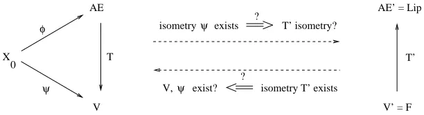
0into some vector space V . Firstly we want to find out under which

embedded isometrically into V and simultaneously V0is isometric isomorphic to F. Both questions will be answered by considering the mapping T of Definition 21 and its adjoint T0. The following treatment will be rather technical, and it might be helpful to have Figure 1 in mind, which shows which relations we want to prove.

X 0

AE’ = Lip

V’ = F T’ exist?

V,ψ

?

isometry T’ exists ?

AE

V

φ

ψ

T

exists T’ isometry? isometry ψ

Figure 1: Relations between Banach spaces and subspaces of Lipschitz functions. The left part

shows the commutative diagram corresponding to the free Banach space property of AE(

X

0). The right part shows the adjoint mapping T0 of T . The dotted arrows in the middle show the relationships we want to investigate.

Now we want to go into detail and start with the first question. For simplicity, we make the following definition.

Definition 23 (Dense isometric embedding) Let(

X

0,d)a metric space and V a normed space. A

mapping Ψ:

X

0→V is called a dense isometric embedding if Ψ is an isometry and if V is the

norm-closure of span_{Ψ(x); x_∈

X

0}.

Lemma 24 (Construction of F for given V ) Let (

X

0,d) be a pointed metric space, (V,_{k · k}V) a

normed space and Ψ:

X

0→V a dense isometric embedding. Then V0 is isomorphic to a closed

subspace F_⊂Lip₀(

X

0), and the canonical injection i : F→Lip0(

X

0)satisfieskik ≤1.

Proof Recall the notation mx :=Φ(x) from Section 3 and analogously denote vx:=Ψ(x). Let

T : AE(

X

0) →V the linear mapping with T◦Φ =Ψ as in Definition 21. As Ψ is an

isome-try, T satisfies _kT_k=1, and maps AE(

X

0) on some dense subspace of V . Consider the adjoint T0: V0_→AE(

X

0)0. It is well known (e.g., Chapter 4 of Rudin, 1991) thatkTk=kT0kand that T0

is injective iff the range of T is dense. Thus, in our case T0 is injective. As by construction also

hT mx,v0i=hT0v0,mxi, we have a unique correspondence between the linear functions in V0 and

some subspace F :=T0V0_⊂AE(

X

0)0: for g∈V0 and f =T0g∈Lip0(

X

0)we have g(vx) = f(mx)

for every x_∈

X

0. The canonical inclusion i corresponds to the adjoint T0.

Lemma 24 shows that the hypothesis space V0constructed by embedding

X

into V is isomorphic to a subset F_⊂Lip₀(

X

0). But it is important to note that this isomorphism is not isometric in general.

Let g_∈V0 and f _∈Lip₀(

X

0)be corresponding functions, that is f =T0g. Because ofkT0k=1 we

know that_kf_kAE0≤ kgk_V, but in general we do not have equality. This means that the marginskgk_V0