Stochastic Composite Likelihood
Joshua V. Dillon [email protected]
Guy Lebanon [email protected]
College of Computing
Georgia Institute of Technology Atlanta, GA, USA
Editor: Fernando Pereira
Abstract
Maximum likelihood estimators are often of limited practical use due to the intensive computation they require. We propose a family of alternative estimators that maximize a stochastic variation of the composite likelihood function. Each of the estimators resolve the computation-accuracy off differently, and taken together they span a continuous spectrum of computation-accuracy trade-off resolutions. We prove the consistency of the estimators, provide formulas for their asymptotic variance, statistical robustness, and computational complexity. We discuss experimental results in the context of Boltzmann machines and conditional random fields. The theoretical and exper-imental studies demonstrate the effectiveness of the estimators when the computational resources are insufficient. They also demonstrate that in some cases reduced computational complexity is associated with robustness thereby increasing statistical accuracy.
Keywords: Markov random fields, composite likelihood, maximum likelihood estimation
1. Introduction
Maximum likelihood estimation is by far the most popular point estimation technique in machine
learning and statistics. Assuming that the data consists of n,m-dimensional vectors
D= (X(1), . . . ,X(n)), X(i)∈Rm, (1)
and is sampled iid from a parametric distribution pθ0 with θ0∈Θ⊂R
r, a maximum likelihood
estimator (MLE) ˆθmln is a maximizer of the log-likelihood function ℓn(θ; D) =
n
∑
i=1
log pθ(X(i)), (2)
ˆ
θml
n =arg max
θ∈Θ ℓn(θ; D).
The use of the MLE is motivated by its consistency,1that is, ˆθmln →θ0as n→∞with probability 1 (Ferguson, 1996). The consistency property ensures that as the number n of samples grows, the
estimator will converge to the true parameterθ0governing the data generation process.
An even stronger motivation for the use of the MLE is that it has an asymptotically normal
distribution with mean vector θ0 and variance matrix (nI(θ0))−1. More formally, we have the
1. The consistency ˆθmln →θ0with probability 1 is sometimes called strong consistency in order to differentiate it from the weaker notion of consistency in probability P(|θˆml
following convergence in distribution as n→∞(Ferguson, 1996)
√ n(θˆml
n −θ0) N(0,I−1(θ0)), (3)
where I(θ)is the r×r Fisher information matrix
I(θ) =Epθ{∇log pθ(X)(∇log pθ(X))⊤}
with∇f representing the r×1 gradient vector of f(θ)with respect toθ. The convergence (3) is espe-cially striking since according to the Cramer-Rao lower bound, the asymptotic variance(nI(θ0))−1 of the MLE is the smallest possible variance for any estimator. Since it achieves the lowest pos-sible asymptotic variance, the MLE (and other estimators which share this property) is said to be asymptotically efficient.
The consistency and asymptotic efficiency of the MLE motivate its use in many circumstances. Unfortunately, in some situations the maximization or even evaluation of the log-likelihood (2) and its derivatives is impossible due to computational considerations. For instance this is the situation in many high dimensional exponential family distributions, including Markov random fields whose graphical structure contains cycles. This has lead to the proposal of alternative estimators under the premise that a loss of asymptotic efficiency is acceptable—in return for reduced computational complexity.
In contrast to asymptotic efficiency, we view consistency as a less negotiable property and prefer to avoid inconsistent estimators if at all possible. This common viewpoint in statistics is somewhat at odds with recent advances in the machine learning literature promoting non-consistent estimators, for example using variational techniques (Jordan et al., 1999). Nevertheless, we feel that there is a consensus regarding the benefits of having consistent estimators over non-consistent ones.
In this paper, we propose a family of estimators, for use in situations where the computation of the MLE is intractable. In contrast to many previously proposed approximate estimators, our estima-tors are statistically consistent and admit a precise quantification of both computational complexity and statistical accuracy through their asymptotic variance. Due to the continuous parameteriza-tion of the estimator family, we obtain an effective framework for achieving a predefined problem-specific balance between computational tractability and statistical accuracy. We also demonstrate that in some cases reduced computational complexity may in fact act as a regularizer, increasing robustness and therefore accomplishing both reduced computation and increased accuracy. This “win-win” situation conflicts with the conventional wisdom stating that moving from the MLE to pseudo likelihood and other related estimators result in a computational win but a statistical loss. Nevertheless we show that this occurs in some practical situations.
For the sake of concreteness, we focus on the case of estimating the parameters associated with Markov random fields. In this case, we provide a detailed discussion of the accuracy-complexity tradeoff. We include experiments on both simulated and real world data for several models in-cluding the Boltzmann machine, conditional random fields, and the Boltzmann linear chain model. Appendix B outlines a road-map of figures and the corresponding exposition.
2. Related Work
technique for approximating expectations and can be used to approximate the normalization term and other intractable portions of the log-likelihood and its gradient (Casella and Robert, 2004). Variational methods are techniques for conducting inference and learning based on tractable bounds (Jordan et al., 1999). A similar approach would be to conduct maximum likelihood estimation for a simpler model that is tractable.
Despite the substantial work on MCMC and variational methods, there are little practical results concerning the convergence and approximation rate of the resulting parameter estimators. Varia-tional techniques are sometimes inconsistent and it is hard to analyze their asymptotic statistical behavior. In the case of MCMC, a number of asymptotic results exist (Casella and Robert, 2004), but since MCMC plays a role inside each gradient descent or EM iteration it is hard to analyze the asymptotic behavior of the resulting parameter estimates. An advantage of our framework is that we are able to directly characterize the asymptotic behavior of the estimator and relate it to the amount of computational savings.
Our work draws on the composite likelihood method for parameter estimation proposed by Lindsay (1988) which in turn generalized the pseudo likelihood of Besag (1974). A selection of more recent studies on pseudo and composite likelihood are Arnold and Strauss (1991), Liang and Yu (2003), Varin and Vidoni (2005), Sutton and McCallum (2007) and Hjort and Varin (2008). Most of the recent studies in this area examine the behavior of the pseudo or composite likelihood in a particular modeling situation. We believe that the present paper is the first to systematically examine statistical and computational tradeoffs in a general quantitative framework. Possible ex-ceptions include the experimental study of texture generation by Zhu and Liu (2002), the work of Xing et al. (2003) which focused on inference rather than parameter estimation, and the examination of generalization performance of small- and large- scale learning systems by Bottou and Bousquet (2008). The work of Liang and Jordan (2008) is also interesting in that the authors employ com-posite likelihood m-estimators and asymptotic arguments to compare the risk of discriminative and generative models. However, our work differs in theme and technique—we explore the tradeoff between computation and accuracy by way of a fundamentally different estimator.
Composite likelihood techniques, and consequently our work, can be thought of as local con-trastive objectives (i.e., pseudo likelihood, concon-trastive divergence). Vickrey et al. (2010) present a non-local alternative in which the objective is not restricted to using the training label, but rather any assignment.
3. Stochastic Composite Likelihood
In many cases, the absence of a closed form expression for the normalization term prevents the computation of the log-likelihood (2) and its derivatives thereby severely limiting the use of the MLE. A popular example is Markov random fields, wherein the computation of the normalization term is often intractable (see Section 6 for more details). In this paper we propose alternative estimators based on the maximization of a stochastic variation of the composite likelihood.
We denote multiple samples using superscripts and individual dimensions using subscripts.
Thus X(jr) refers to the j-dimension of the r sample. Following standard convention we refer to
variable
XS def
={Xi: i∈S}, X−j
def
={Xi: i6= j}. (4)
We start by reviewing the pseudo log-likelihood function (Besag, 1974) associated with the data
D (1),
pℓn(θ; D) def =
n
∑
i=1
m
∑
j=1
log pθ(X(ji)|X−(i)j). (5)
The maximum pseudo likelihood estimator (MPLE) ˆθmpln is consistent, that is, ˆθmpln →θ0with
prob-ability 1, but possesses considerably higher asymptotic variance than the MLE’s(nI(θ0))−1. Its
main advantage is that it does not require the computation of the normalization term as it cancels out in the probability ratio defining conditional distributions
pθ(Xj|X−j) =pθ(Xj|{Xk: k6= j}) =
pθ(X)
∑xj pθ(X1, . . . ,Xj−1,Xj=xj,Xj+1, . . . ,Xm)
.
The MLE and MPLE represent two different ways of resolving the tradeoff between asymptotic variance and computational complexity. The MLE has low asymptotic variance but high computa-tional complexity while the MPLE has higher asymptotic variance but low computacomputa-tional complex-ity. It is desirable to obtain additional estimators realizing alternative resolutions of the accuracy complexity tradeoff. To this end we define the stochastic composite likelihood whose maximization provides a family of consistent estimators with statistical accuracy and computational complexity spanning the entire accuracy-complexity spectrum.
Stochastic composite likelihood generalizes the likelihood and pseudo likelihood functions by constructing an objective function that is a stochastic sum of likelihood objects. We start by defining the notion of m-pairs and likelihood objects and then proceed to stochastic composite likelihood.
Definition 1 An m-pair (A,B) is a pair of sets A,B⊂ {1, . . . ,m} satisfying A6= /0=A∩B. The likelihood object associated with an m-pair(A,B)and X is Sθ(A,B)def=log pθ(XA|XB)where XS is
defined in (4). The composite log-likelihood function (Lindsay, 1988) is a collection of likelihood objects defined by a finite sequence of m-pairs(A1,B1), . . . ,(Ak,Bk)
cℓn(θ; D) def =
n
∑
i=1
k
∑
j=1
log pθ(XA(i)
j|X
(i)
Bj). (6)
There is a certain lack of flexibility associated with the composite likelihood framework as each likelihood object is either selected or not for the entire sample X(1), . . . ,X(n). There is no allowance for some objects to be selected more frequently than others. For example, available computational resources may allow the computation of the log-likelihood for 20% of the samples, and the pseudo likelihood for the remaining 80%. In the case of composite likelihood if we select the full likelihood component (or the pseudo likelihood or any other likelihood object) then this component is applied to all samples indiscriminately.
In SCL, different likelihood objects Sθ(Aj,Bj) may be selected for different samples with the
The selection may be non-coordinated, in which case each component is selected or not indepen-dently of the other components. Or it may be coordinated in which case the selection of one com-ponent depends on the selection of the other ones. For example, we may wish to avoid selecting a
pseudo likelihood component for a certain sample X(i)if the full likelihood component was already
selected for it.
Another important advantage of stochastic selection is that the discrete parameterization of (6) defined by the sequence(A1,B1), . . . ,(Ak,Bk)is less convenient for theoretical analysis. Each
com-ponent is either selected or not, turning the problem of optimally selecting comcom-ponents into a hard combinatorial problem. The stochastic composite likelihood, which is defined below, enjoys contin-uous parameterization leading to more convenient optimization techniques and convergence analy-sis.
Definition 2 Consider a finite sequence of m-pairs(A1,B1), . . . ,(Ak,Bk), a data set D= (X(1), . . . ,
X(n)),β∈Rk+, and n iid, length k, binary random vectors Z(1), . . . ,Z(n)
i.i.d.
∼P(Z)withλj def
=E(Zj)>0.
The stochastic composite log-likelihood (SCL) is
scℓn(θ; D,Z)def=1
n
n
∑
i=1
mθ(X(i),Z(i)), where
mθ(X,Z)def= k
∑
j=1
βjZjlog pθ(XAj|XBj), (7)
where, for brevity, we typically omit D,Z in favor of scℓn(θ).
In other words, the SCL is a stochastic extension of (6) where for each sample X(i),i=1, . . . ,n, the
likelihood objects S(A1,B1), . . . ,S(Ak,Bk)are either selected or not, depending on the values of the
binary random variables Z1(i), . . . ,Zk(i)and weighted by the constantsβ1, . . . ,βk. Note that Z(ji)may
in general depend on Zr(i)but not on Zr(l)or on X(i).
When we focus on examining different models for P(Z) we sometimes parameterize it, for
example byλ, that is, Pλ(Z). This reuse ofλ(it is also used in Definition 2) is a notational abuse. We accept it, however, as in most of the cases that we considerλ1, . . . ,λk from Definition 2 either
form the parameter vector for P(Z)or are part of it. Often we refer to a particularλas a “policy” in order to emphasize its role as a “knob” in selecting particular m-pairs.
Some illustrative examples follow.
Independence. Factorizing Pλ(Z1, . . . ,Zk) =∏jPλj(Zj)leads to Z
(i)
j ∼Ber(λj)with complete
in-dependence among the indicator variables. For each sample X(i), each likelihood object
S(Aj,Bj)is selected or not independently with probabilityλj.
Multinomial. A multinomial model Z∼Mult(1,λ) implies that for each sample Z(i)a multivari-ate Bernoulli experiment is conducted with precisely one likelihood object being selected depending on the selection probabilitiesλ1, . . . ,λk.
Product of Multinomials. A product of multinomials is formed by a partition of the dimensions to
l disjoint subsets{1, . . . ,m}=C1∪ ···Clwhere ZCi∼Mult(1,(λj: j∈Ci)), that is,
P(Z) = c
∏
i=1
Loglinear Models. The distribution P(Z) follows a hierarchical loglinear model (Bishop et al., 1975). This case subsumes the other cases above.
In analogy to the MLE and the MPLE, the maximum SCL estimator (MSCLE) ˆθmsln estimates
θ0 by maximizing the SCL function. In contrast to the log-likelihood and pseudo log-likelihood
functions, the SCL function and its maximizer are random variables that depend on the indica-tor variables Z(1), . . . ,Z(n) in addition to the data D. As such, its behavior should be summarized
by examining the limit n→∞. Doing so eliminates the dependency on particular realizations of
Z(1), . . . ,Z(n) in favor of the the expected frequencies λj =EP(Z)Zj which are non-random
con-stants.
The statistical accuracy and computational complexity of the SCL estimator are continuous
functions of the parameters (β,λ) (component weights and selection probabilities respectively)
which vary continuously throughout their domain (λ,β)∈Λ×Rk
+. Choosing appropriate values
of(λ,β)retrieves the special cases of MLE, MPLE, maximum composite likelihood with each
se-lection being associated with a distinct statistical accuracy and computational complexity. The SCL
framework allows selections of many more values of(λ,β)realizing a wide continuous spectrum of
estimators, each resolving the accuracy-complexity tradeoff differently.
We include below a demonstration of the SCL framework in a simple low dimensional case. In the following sections we discuss in detail the statistical behavior of the MSCLE and its computa-tional complexity. We conclude the paper with several experimental studies.
3.1 Boltzmann Machine Example
Before proceeding we illustrate the SCL framework using a simple example involving a Boltzmann machine (Hinton and Sejnowski, 1983). Section 8.1 describes the specifics of this model. We con-sider in detail three SCL policies: full likelihood (FL), pseudo likelihood (PL), and a stochastic
combination of first and second order pseudo likelihood with the first order components p(Xi|X−i)
selected with probabilityλand the second order components p(Xi,Xj|X{i,j}c)selected with
proba-bility 1−λ.
Denoting the number of (binary) graph vertices, or nodes, by m, and the number of examples by
n, the computational complexity of the FL function measured in FLOP2counts is O m2(2m+n)
(for the log-likelihood) and O m22
2m+n m
2
for the log-likelihood gradient.3 The exponential
growth in m prevents such computations for large graphs.
The k-order PL function offers a practical alternative to FL (1-order PL corresponds to the tradi-tional pseudo likelihood and 2-order PL its analog, p(X{i,j}|X{i,j}c)). The complexity of computing
the corresponding SCL function is O m2
( mk
2k+n)
for the objective function and O m22 m
k
2k+
n m2for its gradient. The slower complexity growth of the k-order PL (polynomial in m instead
of exponential) is offset by its reduced statistical accuracy, which we measure using the normalized asymptotic variance
eff(θˆn) = det(Asymp Var(θˆn))
det(Asymp Var(θˆml
n ))
(8)
2. FLOP is the number of FLoating point OPerations.
3. With memoization the complexity of the gradient can be reduced to O m2
2m+n m2
which is bounded from below by 1 (due to Cramer Rao lower bound) and its deviation from 1 reflects its inefficiency relative to the MLE.
The MLE thus achieves the best accuracy but it is computationally intractable. The first order and second order PL have higher asymptotic variance but are easier to compute. The SCL frame-work enables adding many more estimators filling in the gaps between ML, 1-order PL, 2-order PL, etc.
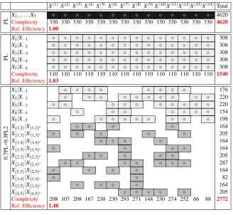
We illustrate three SCL functions in the context of a simple Boltzmann machine (five binary nodes, fourteen samples X(1), . . . ,X(14),θtrue= (−1,−1,−1,−1,−1,1,1,1,1,1)) in Figure 1. The top box refers to the full likelihood policy, that is, maximum likelihood. For each of the fourteen samples, the FL component is computed and their aggregation forms the SCL function which in this case equals the log-likelihood. The selection of the FL component for each sample is illustrated using a diamond box. The values under the boxes reflect the FLOP counts needed to compute the components and the total complexity associated with computing the entire SCL or log-likelihood is listed on the right. As mentioned above, the normalized asymptotic variance (8) is 1.
The pseudo likelihood function (5) is illustrated in the second box where each row correspond to one of the five PL components. As each of the five PL component is selected for each of the samples
we have diamond boxes covering the entire 5×14 array. The shade of the diamond boxes reflects
the complexity required to compute them enabling an easy comparison to the FL components in the top of the figure (note how the FL boxes are much darker than the PL boxes). The numbers at the bottom of each column reflect the FLOP marginal count for each of the fourteen samples and the numbers to the right of the rows reflect the FLOP marginal count for each of the PL components. In this case the FLOP count is less than half the FLOP count of the FL in top box (this reduction in complexity obtained by replacing FL with PL will increase dramatically for graphs with more than
5 nodes) but the asymptotic variance is 83% higher.4
The third SCL policy reflects a stochastic combination of first and second order pseudo
likeli-hood components. Each first order component is selected with probabilityλand each second order
component is selected with probability 1−λ. The result is a collection of 5 1-order PL components
and 10 2-order components with only some of them selected for each of the fourteen samples. Again diamond boxes correspond to selected components which are shaded according to their FLOP com-plexity. The per-component FLOP marginals and per example FLOP marginals are listed as the bottom row and right-most column. The total complexity is somewhere between FL and PL and the asymptotic variance is reduced from the PL’s 183% to 148%.
Additional insight may be gained at this point by considering Figure 3 which plots several SCL estimators as points in the plane whose x and y coordinates correspond to normalized asymptotic variance and computational complexity respectively. We turn at this point to considering the statis-tical properties of the SCL estimators.
4. Consistency and Asymptotic Variance of ˆθmsln
A nice property of the SCL framework is enabling mathematical characterization of the statistical
properties of the estimator ˆθmsln . In this section we examine the conditions for consistency of the
MSCLE and its asymptotic distribution and in the next section we consider robustness. The propo-sitions below constitute novel generalizations of some well-known results in classical statistics.
Proofs may be found in Appendix A. For simplicity, we assume that X is discrete and pθ(x)>0.
X(1)X(2)X(3)X(4) X(5) X(6) X(7) X(8) X(9)X(10)X(11)X(12)X(13)X(14) Total
F
L ComplexityX1, , . . . ,X5 330 330 330 330 330 330 330 330 330 330 330 330 330 330⋄ ⋄ ⋄ ⋄ ⋄ ⋄ ⋄ ⋄ ⋄ ⋄ ⋄ ⋄ ⋄ ⋄ 46204620
Rel. Efficiency 1.00
P
L
X1|X−1 ⋄ ⋄ ⋄ ⋄ ⋄ ⋄ ⋄ ⋄ ⋄ ⋄ ⋄ ⋄ ⋄ ⋄ 308
X2|X−2 ⋄ ⋄ ⋄ ⋄ ⋄ ⋄ ⋄ ⋄ ⋄ ⋄ ⋄ ⋄ ⋄ ⋄ 308
X3|X−3 ⋄ ⋄ ⋄ ⋄ ⋄ ⋄ ⋄ ⋄ ⋄ ⋄ ⋄ ⋄ ⋄ ⋄ 308
X4|X−4 ⋄ ⋄ ⋄ ⋄ ⋄ ⋄ ⋄ ⋄ ⋄ ⋄ ⋄ ⋄ ⋄ ⋄ 308
X5|X−5 ⋄ ⋄ ⋄ ⋄ ⋄ ⋄ ⋄ ⋄ ⋄ ⋄ ⋄ ⋄ ⋄ ⋄ 308
Complexity 110 110 110 110 110 110 110 110 110 110 110 110 110 110 1540
Rel. Efficiency 1.83
0
.7
P
L
+
0
.3
P
L
2
X1|X−1 ⋄ ⋄ ⋄ ⋄ ⋄ ⋄ ⋄ ⋄ 176
X2|X−2 ⋄ ⋄ ⋄ ⋄ ⋄ ⋄ ⋄ ⋄ ⋄ ⋄ 220
X3|X−3 ⋄ ⋄ ⋄ ⋄ ⋄ ⋄ ⋄ ⋄ ⋄ ⋄ 220
X4|X−4 ⋄ ⋄ ⋄ ⋄ ⋄ ⋄ ⋄ 154
X5|X−5 ⋄ ⋄ ⋄ ⋄ ⋄ ⋄ ⋄ ⋄ ⋄ 198
X{1,2}|X{1,2}c ⋄ ⋄ ⋄ ⋄ 164
X{1,3}|X{1,3}c ⋄ ⋄ ⋄ ⋄ ⋄ 205
X{1,4}|X{1,4}c ⋄ ⋄ ⋄ ⋄ 164
X{1,5}|X{1,5}c ⋄ ⋄ ⋄ ⋄ 164
X{2,3}|X{2,3}c ⋄ ⋄ ⋄ ⋄ ⋄ 205
X{2,4}|X{2,4}c ⋄ ⋄ ⋄ ⋄ ⋄ ⋄ ⋄ 287
X{2,5}|X{2,5}c ⋄ ⋄ ⋄ ⋄ 164
X{3,4}|X{3,4}c ⋄ ⋄ 82
X{3,5}|X{3,5}c ⋄ ⋄ ⋄ ⋄ 164
X{4,5}|X{4,5}c ⋄ ⋄ ⋄ ⋄ ⋄ 205
Complexity 208 107 208 167 230 230 293 271 148 230 274 252 66 88 2772
Rel. Efficiency 1.48
Figure 1: Sample runs of three different SCL policies for 14 examples X(1), . . . ,X(14)drawn from a 5 binary node Boltzmann machine (θtrue= (−1,−1,−1,−1,−1,1,1,1,1,1)). The poli-cies are full likelihood (FL, top), pseudo likelihood (PL, middle), and a stochastic combi-nation of first and second order pseudo likelihood with the first order components selected with probability 0.7 and the second order components with probability 0.3 (bottom).
The sample runs for the policies are illustrated by placing a diamond box in table entries corresponding to selected likelihood objects (rows corresponding to likelihood objects
and columns to X(1), . . . ,X(14)). The FLOP counts of each likelihood object determines
the shade of the diamond boxes while the total FLOP counts per example and per like-lihood objects are displayed as table marginals (bottom row and right column for each policy). We also display the total FLOP count and the normalized asymptotic variance (8).
Even in the simple case of 5 nodes, FL is the most complex policy with PL requiring a third of the FL computation. 0.7PL+0.3PL2 is somewhere in between. The situation is reversed for the estimation accuracy-FL achieves the lowest possible normalized asymp-totic variance of 1, PL is almost twice that, and 0.7PL+0.3PL2 somewhere in the middle.
The SCL framework spans the accuracy-complexity spectrum. Choosing the rightλvalue
Definition 3 A sequence of m-pairs(A1,B1), . . . ,(Ak,Bk)is m-pair identifiable, or simply
identifi-able, of pθif the map{pθ(XAj|XBj): j=1, . . . ,k} 7→pθ(X)is injective. In other words, there exists
only a single collection of conditionals{pθ(XAj|XBj): j=1, . . . ,k}that does not contradict the joint
pθ(X).
Proposition 1 Let Θ⊂ Rr be an open set, pθ(x) >0 and continuous and smooth in θ, and
(A1,B1), . . . ,(Ak,Bk) be a sequence of m-pairs for which {(Aj,Bj):∀j such thatλj >0} ensures
identifiability. Then the sequence of SCL maximizers is strongly consistent, that is,
P
lim
n→∞
ˆ
θn=θ0
=1.
The above proposition indicates that to guarantee consistency, the sequence of m-pairs needs to satisfy Definition 3. It can be shown that a selection equivalent to the pseudo likelihood function, that is,
S
={(A1,B1), . . . ,(Am,Bm)} where Ai={i},Bi={1, . . . ,m} \Ai (9)ensures identifiability and consequently the consistency of the MSCLE estimator. Furthermore,
every selection of m-pairs that subsumes
S
in (9) similarly guarantees identifiability and consistency.The proposition below establishes the asymptotic normality of the MSCLE ˆθn. The asymptotic
variance enables the comparison of SCL functions with different parameterizations(λ,β).
Proposition 2 Making the assumptions of Proposition 1 as well as convexity ofΘ⊂Rrwe have the following convergence in distribution
√
n(θˆmsln −θ0) N(0,ϒΣϒ)
where
ϒ−1=
∑
kj=1
βjλjVarθ0(∇Sθ0(Aj,Bj)),
Σ=Varθ0
k
∑
j=1
βjλj∇Sθ0(Aj,Bj) !
.
The notationVarθ0(Y)represents the covariance matrix of the random vector Y under pθ0 while the
notations →p , in the proof below denote convergences in probability and in distribution
(Fergu-son, 1996).∇represents the gradient vector with respect toθ.
Whenθis a vector the asymptotic variance is a matrix. To facilitate comparison between
dif-ferent estimators we follow the convention of using the determinant, and in some cases the trace, to measure the statistical accuracy. See Chapter 4 of Serfling (1980) for some heuristic arguments for doing so. Figures 1,2,3 provide the asymptotic variance for some SCL estimators and describe how it can be used to gain insight into which estimator to use.
The fact that√n(θˆn−θ0)converges in distribution to a Gaussian with zero mean (for the MLE and similarly for SCL estimators as we show above) implies that the estimator’s asymptotic
behav-ior, up to n−1/2 order, is determined exclusively by the asymptotic variance. That means that the
Taylor series with more terms) show that the bias decays in the faster rate of n−1 (Cox and Snell, 1968). We thus follow the statistical convention of conducting first order asymptotic analysis and concentrate on the estimator’s asymptotic variance.
The statistical accuracy of the SCL estimator depends onβ(weight parameters) andλ(selection
parameter). It is thus desirable to use the results in this section in determining what values ofβ,λto use. Directly using the asymptotic variance is not possible in practice as it depends on the unknown
quantityθ0. However, it is possible to estimate the asymptotic variance using the training data. We
describe this in Section 7.
5. Robustness of ˆθmsln
We observed in our experiments (see Section 8) that the SCL estimator sometimes performed better on a held-out test set than did the maximum likelihood estimator. This phenomenon seems to be in contradiction to the fact that the asymptotic variance of the MLE is lower than that of the SCL maximizer. This is explained by the fact that in some cases the true model generating the data
does not lie within the parametric family {pθ:θ∈Θ} under consideration. For example, many
graphical models (HMM, CRF, LDA, etc.) make conditional independence assumptions that are often violated in practice. In such cases the SCL estimator acts as a regularizer achieving better test set performance than the non-regularized MLE. We provide below a theoretical account of this phenomenon using the language of m-estimators and statistical robustness. Our notation follows the one in van der Vaart (1998).
We assume that the model generating the data is outside the model family P(X)6∈ {pθ:θ∈Θ}
and we extend the notation of mθ(X,Z)in (7) with,
ψθ(X,Z)=def∇mθ(X,Z), ˙
ψθ(X,Z)=def∇2m
θ(X,Z), and
Ψn(θ)=def 1
n
n
∑
i=1
ψθ(X(i),Z(i)),
noting that ˙ψθ(X,Z)is a matrix of second order derivatives.
Proposition 3 below generalizes the consistency result by asserting that ˆθn→θ0whereθ0is the point on{pθ:θ∈Θ}that is closest to the true model P, as defined by
θ0=arg max
θ∈Θ M(θ) where M(θ)
def
= −
k
∑
j=1
βjλjD(P(XAj|XBj)||pθ(XAj|XBj)),
or equivalently,θ0satisfies
EP(X)EP(Z)ψθ0(X,Z) =0.
When the SCL function reverts to the log-likelihood function,θ0becomes the KL projection of the
true model P onto the parametric family{pθ:θ∈Θ}.
Proposition 3 Assuming the conditions in Proposition 1 as well as supθ:kθ−θ0k≥εM(θ)<M(θ0)for
The added condition maintains thatθ0is a well separated maximum point of M. In other words
it asserts that only values close toθ0 may yield a value of M that is close to the maximum M(θ0).
This condition is satisfied in the case of most exponential family models.
Proposition 4 Assuming the conditions of Proposition 2 as well asEP(X)EP(Z)kψθ0(X,Z)k2<∞,
EP(X)EP(Z)ψ˙θ0(X)exists and is non-singular,|Ψ¨i j|=|∂2ψθ(x)/∂θiθj|<g(x)for all i,j andθin a
neighborhood ofθ0for some integrable g, we have
√
n(θˆn−θ0) =−(EP(X)EP(Z)ψ˙θ0)−
1√1
n
n
∑
i=1
ψθ0(X
(i),Z(i)) +o
P(1) (10)
or equivalently
ˆ
θn=θ0−(EP(X)EP(Z)ψ˙θ0)−
11
n
n
∑
i=1
ψθ0(X
(i),Z(i)) +o
P
1
√ n
. (11)
Above, fn=oP(gn)means fn/gnconverges to 0 with probability 1.
Corollary 1 Assuming the conditions specified in Proposition 4 we have
√
n(θˆn−θ0) N(0,(EP(X)EP(Z)ψ˙θ0)−
1(
EP(X)EP(Z)ψθ0ψ⊤θ0)(EP(X)EP(Z)ψ˙θ0)−
1). (12)
Equation (11) means that asymptotically, ˆθn behaves as θ0 plus the average of iid RVs. As
mentioned in van der Vaart (1998) this fact may be used to obtain a convenient expression for the asymptotic influence function, which measures the effect of adding a new observation to an existing large data set. Neglecting the remainder in (10) we have
I
(x,z)=defθˆn(X(1), . . . ,X(n−1),x,Z(1), . . . ,Z(n−1),z)−θˆn−1(X(1), . . . ,X(n−1),Z(1), . . . ,Z(n−1))≈ −(EP(X)EP(Z)ψ˙θ0)−1 1
n
n−1
∑
i=1
ψθ0(X
(i),Z(i)) +1
nψθ0(w,z)−
1
n−1
n−1
∑
i=1
ψθ0(X
(i),Z(i))
!
=−(EP(X)EP(Z)ψ˙θ0)−11
nψθ0(w,z) + (EP(X)EP(Z)ψ˙θ0)−
1 1
n(n−1) n−1
∑
i=1
ψθ0(X
(i),Z(i))
=−1
n(EP(X)EP(Z)ψ˙θ0)−
1ψ
θ0(w,z) +oP
1
n
. (13)
Corollary 1 and Equation (13) measure the statistical behavior of the estimator when the true distribution is outside the model family. In these cases it is possible that a computationally effi-cient SCL maximizer will result in higher statistical accuracy as well. This “win-win” situation of improving in both accuracy and complexity over the MLE is confirmed by our experiments in Section 8.
We finally note that the above analysis is not limited to misspecified models. For example, the influence function may be used to detect the robustness of ˆθnto outliers or rare events (it is desirable
6. Stochastic Composite Likelihood for Markov Random Fields
Markov random fields (MRF) are some of the more popular statistical models for complex high dimensional data. Approaches based on pseudo likelihood and composite likelihood are naturally well-suited in this case due to the cancellation of the normalization term in the probability ratios
defining conditional distributions. More specifically, a MRF with respect to a graph G= (V,E),
V ={1, . . . ,m}with a clique set
C
is given by the following exponential family modelpθ(x) =exp
∑
C∈C
θCfC(xC)−log Z(θ) !
,
Z(θ) =
∑
xexp
∑
C∈C
θcfC(xC) !
. (14)
The primary bottlenecks in obtaining the maximum likelihood are the computations log Z(θ)and
∇log Z(θ). Their computational complexity is exponential in the graph’s treewidth and for many
cyclic graphs, such as the Ising model or the Boltzmann machine, it is exponential in|V|=m.
In contrast, the conditional distributions that form the composite likelihood of (14) are given by (note the cancellation of Z(θ))
pθ(xA|xB) = ∑ x′
(A∪B)c
exp
∑C∈CθCfC((xA,xB,x′(A∪B)c)C)
∑ x′(A∪B)c
∑ x′′A
exp
∑ C∈C
θCfC((x′′A,xB,x′(A∪B)c)C)
. (15)
whose computation is substantially faster. Specifically, The computation of (15) depends on the size of the sets A and(A∪B)c and their intersections with the cliques in
C
. In general, selecting small|Aj|and Bj= (Aj)c leads to efficient computation of the composite likelihood and its gradient. For
example, in the case of|Aj|=l,|Bj|=m−l with l≪m we have that k≤m!/(l!(m−l)!)and the
complexity of computing the cℓ(θ)function and its gradient may be shown to require time that is at
most exponential in l and polynomial in m.
7. Automatic Selection ofβ
As Proposition 2 indicates, the weight vectorβand selection probabilitiesλplay an important role
in the statistical accuracy of the estimator through its asymptotic variance. The computational
com-plexity, on the other hand, is determined byλindependently ofβ. Conceptually, we are interested in
resolving the accuracy-complexity tradeoff jointly for bothβ,λbefore estimatingθby maximizing
the SCL function. However, since the computational complexity depends only onλwe propose the
following simplified problem: Selectλbased on available computational resources, and then given
λ, select theβ(andθ) that will achieve optimal statistical accuracy.
Selectingβthat minimizes the asymptotic variance is somewhat ambiguous asϒΣϒin
Proposi-tion 2 is an r×r positive semidefinite matrix. A common solution is to consider the determinant as
a one dimensional measure of the size of the variance matrix,5and minimize
J(β) =log det(ϒΣϒ) =log detΣ+2 log detϒ. (16)
A major complication with selecting βbased on the optimization of (16) is that it depends on
the true parameter valueθ0which is not known at training time. This may be resolved, however,
by noting that (16) is composed of covariance matrices under θ0 which may be estimated using
empirical covariances over the training set. To facilitate fast computation of the optimalβwe also
propose to replace the determinant in (16) with the product of the diagonal elements. Such an approximation is motivated by Hadamard’s inequality (which states that for symmetric matrices
det(M)≤∏iMii) and by Gerˇsgorin’s circle theorem (see below). This approximation works well in
practice as we observe in the experiments section. We also note that the procedure described below involves only simple statistics that may be computed on the fly and does not contribute significant additional computation (nor do they require significant memory).
More specifically, we denote K(i j)=Covθ0(∇Sθ0(Ai,Bi),∇Sθ0(Aj,Bj))with entries K
(i j)
st , and
approximate the log det terms in (16) using
log detϒ=−log det
k
∑
j=1
βjλjK(j j)≈ − r
∑
l=1 log
k
∑
j=1
βjλjK( j j)
ll
log detΣ=log detVarθ0 k
∑
j=1
βjλj∇Sθ0(Aj,Bj) !
=log det
k
∑
i=1
k
∑
j=1
βiλiβjλjK(i j)
≈
r
∑
l=1 log
k
∑
i=1
k
∑
j=1
βiλiβjλjKll(i j).
We denote (assuming A is a n×n matrix) for i ∈ {1, . . . ,n}, Ri(A) = ∑j6=i Ai j
and let
D(Aii,Ri(A))(Diwhere unambiguous) be the closed disc centered at Aiiwith radius Ri(A). Such a
disc is called a Gerˇsgorin disc. The result below states that for matrices that are close to diagonal, the eigenvalues are close to the diagonal elements making our approximation accurate.
Theorem 1 (Gerˇsgorin’s circle theorem, for example, Horn and Johnson, 1990) Every eigen-value of A lies within at least one of the Gerˇsgorin discs D(Aii,Ri(A)).Furthermore, if the union of
k discs is disjoint from the union of the remaining n−k discs, then the former union contains exactly k and the latter n−k eigenvalues of A.
Algorithm 1 solves for θ,β jointly using alternating optimization. The second optimization
problem J(β;·)is done using the approximation above and may be computed with minimal
addi-tional computation. The components of this objective are typically freely available when scℓ is
minimized with Newton-type methods. In practice we found that such an approach leads to a
selec-tion ofβthat is close to optimal, despite loose convergence criteria for the minimization of the scℓ
objective (see Sec. 8.3 and Figures 14, 20 for results).
8. Experiments
We demonstrate the asymptotic properties of ˆθmsln and explore the complexity-accuracy tradeoff for
three different models-Boltzmann machine, linear Boltzmann MRF and conditional random fields. In terms of data sets, we consider synthetic data as well as data sets from sentiment prediction and text chunking domains.
In Appendix B we list all figures by subject. The basic road-map is to explore SCL for a theoret-ical Boltzmann machine and then to explore two data sets using both generative and discriminative
Algorithm 1 Calculate ˆθmsl
Require: {Xi}i∈Iandλ,β(0)
1: t←1
2: while t<MAXITS do
3: θ(t)←arg min scℓ(θ;{Xi}i∈I,λ,β(t−1)) 4: if converged then
5: return θ
6: end if
7: β(t)←arg min J(β;{K(i j)}(i,j)∈J,λ,θ)
8: t←t+1
9: end while
10: return false
8.1 Toy Example: Boltzmann Machines
We illustrate the improvement in asymptotic variance of the MSCLE associated with adding higher order Boltzmann machine likelihood components with increasingly higher probability. The Boltz-mann machine can be parameterized as,
pθ(x) =exp
∑
i<j
θi jxixj−logψ(θ) !
, x∈ {0,1}m.
To be able to accurately compute the asymptotic variance we use m=5 withθbeing a 52
dimen-sional vector with half the components+1 and half−1. Since the asymptotic variance of ˆθmsln is a
matrix we summarize its size using either its trace or determinant.
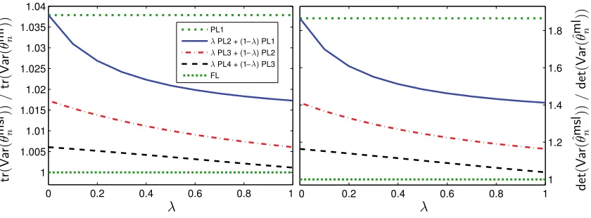
Figure 2 displays the asymptotic variance, relative to the minimal variance of the MLE, for the
cases of full likelihood (FL), pseudo likelihood (|Aj|=1) PL1, stochastic combination of pseudo
likelihood and 2nd order pseudo likelihood (|Aj|=2) componentsλPL2+ (1−λ)PL1, stochastic
combination of 2nd order pseudo likelihood and 3rd order pseudo likelihood (|Aj|=3) components
λPL3+(1−λ)PL2, and stochastic combination of 3rd order pseudo likelihood and 4th order pseudo
likelihood (|Aj|=4) componentsλPL4+ (1−λ)PL3.
The graph demonstrates the computation-accuracy tradeoff as follows: (a) pseudo likelihood is the fastest but also the least accurate, (b) full likelihood is the slowest but the most accurate, (c) adding higher order components reduces the asymptotic variance but also requires more
computa-tion, (d) the variance reduces with the increase in the selection probability λof the higher order
component, and (e) adding 4th order components brings the variance very close the lower limit and with each successive improvement becoming smaller and smaller according to a law of diminishing returns.
Figure 3 displays the asymptotic accuracy and complexity for different SCL policies for m=9
binary valued vertices of a Boltzmann machine. We explore three polices in which we denote pseudo
likelihood components of size, or order, k. These policies include: λ1β1PL1+λ2(1−β1)PL2,
0 0.2 0.4 0.6 0.8 1 1
1.005 1.01 1.015 1.02 1.025 1.03 1.035 1.04
0 0.2 0.4 0.6 0.8 1
1 1.2 1.4 1.6 1.8 PL1
PL2 + (1 ) PL1
PL3 + (1 ) PL2
PL4 + (1 ) PL3
FL
Figure 2: Asymptotic variance matrix, as measured by trace (left) and determinant (right), as a function of the selection probabilities for different stochastic versions of the SCL func-tion.
lie to the right and top of that boundary may be improved by selecting a policy below and to the left of it.
8.2 Local Sentiment Prediction
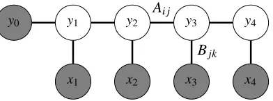
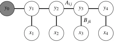
Our first real world data set experiment involves local sentiment prediction using a conditional MRF model. The data set consisted of 249 movie review documents having an average of 30.5 sentences each with an average of 12.3 words from a 12633 word vocabulary. Each sentence was manually labeled as one of five sentimental designations: very negative, negative, objective, positive, or very positive. As described in Mao and Lebanon (2007) (where more information may be found) we considered the task of predicting the local sentiment flow within these documents using regularized conditional random fields (CRFs) (see Figure 4 for a graphical diagram of the model in the case of four sentences).
As is common practice, we curtail overfitting through a L2regularizer, exp{−(2nσ2)−1||θ||2 2},
which is strong whenσ2is small and weak whenσ2is large. We considerσ2a hyper-parameter and
select it through cross-validation, unless noted otherwise.
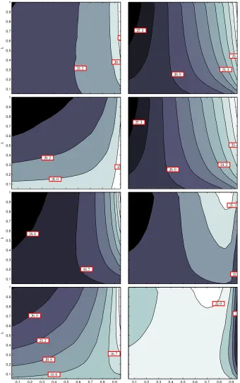
Figure 5 shows the contour plots of train and test log-likelihood as a function of the SCL
param-eters: weightβand selection probability λ. The likelihood components were mixtures of full and
pseudo (|Aj|=1) likelihood (rows 1,3) and pseudo and 2nd order pseudo(|Aj|=2) likelihood (rows
2,4). Aj identifies a set of labels corresponding to adjacent sentences over which the probabilistic
1.030 1.04 1.05 1.06 1.07 1.08 0.2
0.4 0.6 0.8 1 1.2 1.4 1.6 1.8
2x 10
4
Normalized Asymptotic Variance
Complexity (FLOP)
♦λ1β1PL1+λ2(1-β1)PL2
λ1β1PL1+λ2(1-β1)PL3
⋆⋆λ1β1PL2+λ2(1-β1)PL3
PL1 PL2
Figure 3: Computation-accuracy diagram for three SCL families:λ1β1PL1+λ2(1−β1)PL2,
λ1β1PL1+λ2(1−β1)PL3, λ1β1PL2+λ2(1−β1)PL3 (for multiple values ofλ1,λ2,β1) for the Boltzmann machine with 9 binary nodes. The pure policies PL1 and PL2 are in-dicated by black circles and the computational complexity of the full likelihood inin-dicated by a dashed line (corresponding normalized asymptotic variance is 1). The PL3 pure pol-icy is beyond the scale of the diagram. As the graph size increases, the computational cost increases dramatically, in particular for the full likelihood policy and to a lesser extent for the pseudo likelihood policy.
decreasing the influence of full likelihood in favor of pseudo likelihood. The fact that this happens
for (relatively) weak regularization,σ2=10, and indicates that lower order pseudo likelihood has a
regularization effect which improves prediction accuracy when the model is not regularized enough. We have encountered this phenomenon in other experiments as well and we will discuss it further in the following subsections.
Figure 6 displays the complexity and negative log-likelihoods (left:train, right:test) of
differ-ent SCL estimators, sweeping throughλandβ, as points in a two dimensional space. The shaded
y0 y1
x1
y2
x2
y3
Ai j
x3
Bjk
y4
x4
Figure 4: Graphical representation of a four token conditional random field (CRF). A, B are weight matrices and represent state-to-state transitions and state-to-observation outputs. Shad-ing indicates the variable is conditioned upon while no shadShad-ing indicates the variable is generated by the model.
achievable region with the exact position on that boundary depending on the required solution of the computation-accuracy tradeoff.
8.3 Text Chunking
This experiment consists of using sequential MRFs to divide sentences into “text chunks,” that is, syntactically correlated sub-sequences, such as noun and verb phrases. Chunking is a crucial step
towards full parsing. For example,6the sentence:
He reckons the current account deficit will narrow to only # 1.8 billion in September.
could be divided as:
[NPHe] [VPreckons] [NPthe current account deficit] [VPwill narrow] [PPto] [NPonly #
1.8 billion] [PPin] [NPSeptember].
where NP, VP, and PP indicate noun phrase, verb phrase, and prepositional phrase.
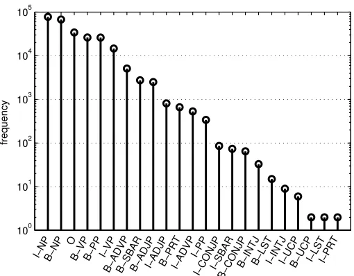
We used the publicly available CoNLL-2000 shared task data set. It consists of labeled partitions of a subset of the Wall Street Journal (WSJ) corpus. Our training sets consisted of sampling 100 sentences without replacement from the the CoNLL-2000 training set (211,727 tokens from WSJ Sections 15-18). The test set was the same as the CoNLL-2000 testing partition (47,377 tokens from WSJ Section 20). Each of the possible 21,589 tokens, that is, words, numbers, punctuation, etc., are tagged by one of 11 chunk types and an O label indicating the token is not part of any chunk. Chunk labels are prepended with flags indicating that the token begins (B-) or is inside (I-) the phrase. Figure 7 lists all labels and respective frequencies. In addition to labeled tokens, the data set contains a part-of-speech (POS) column. These tags were automatically generated by the Brill tagger and must be incorporated into any model/feature set accordingly.
In the following, we explore this task using various SCL selection policies on two related, but fundamentally different sequential MRFs: Boltzmann chain MRFs and CRFs.
8.3.1 BOLTZMANNCHAINMRF
Boltzmann chains are a generative MRF that are closely related to hidden Markov models (HMM). See MacKay (1996) for a discussion on the relationship between Boltzmann chain MRFs and
1
20. 8 23. 2
λ
0.1 0.2 0.3 0.4 0.5 0.6 0.7 0.8 0.9
23. 3
24. 3 26. 0
27. 3
23.
26. 0 29. 2
λ
0.1 0.2 0.3 0.4 0.5 0.6 0.7 0.8 0.9 1
23. 3
24. 3 26. 0
27. 3
16. 7 18. 6
λ
0.1 0.2 0.3 0.4 0.5 0.6 0.7 0.8 0.9 1
21. 3
22.
16. 7
18. 6 20. 8 23. 2 26. 0
β
λ
0.1 0.2 0.3 0.4 0.5 0.6 0.7 0.8 0.9
0.1 0.2 0.3 0.4 0.5 0.6 0.7 0.8 0.9 1
22. 0
23
β
0.1 0.2 0.3 0.4 0.5 0.6 0.7 0.8 0.9
Figure 5: Train (left column) and test (right column) neg. log-likelihood contours for maximum SCL estimators for the CRF model. L2 regularization, exp{−(2nσ2)−1||θ||22},
parame-ters areσ2=1 (rows 1,2) andσ2=10 (rows 3,4). Rows 1,3 are stochastic mixtures of
Figure 6: Scatter plot representing complexity and negative log-likelihood (left:train, right:test) of
SCL functions for CRFs with L2 regularization parameterσ2=1/2. The points represent
different stochastic combinations of full and pseudo likelihood components. The shaded region represents impossible accuracy/complexity demands. Since the boundary of the obtainable region is empirical, the optimal beta always lies on this boundary. By varying
λ,βwe are able to smoothly span complexity (wall seconds) and accuracy.
100
101
102
103
104
105
I−NPB−NP O
B−VPB−PP I−VP
B−ADVPB−SBARB−ADJPI−ADJPB−PRTI−ADVP
I−PP
I−CONJPI−SBARB−CONJPB−INTJB−LSTI−INTJI−UCPB−UCP
I−LSTI−PRT
frequency
HMMs. We consider SCL components of the form p(X2,Y2|Y1,Y3), p(X2,X3,Y2,Y3|Y1,Y4) which we refer to as first and second order pseudo likelihood (with higher order components generalizing in a straightforward manner).
y0 y1
x1
y2
x2
y3 Ai j
x3 Bjk
y4
x4
Figure 8: Graphical representation of a four token Boltzmann chain. A, B are weight matrices and represent preference in particular state-to-state transitions and state-to-feature emissions. Only the start state is conditioned upon while all others are generative.
The nature of the Boltzmann chain constrains our feature set to only encode the particular token present at each position, or time index. In doing so we avoid having to model additional depen-dencies across time steps and dramatically reduce computational complexity. Although SCL is precisely motivated by high treewidth graphs, we wish to include the full likelihood for demonstra-tive purposes—in practice, this is often not possible. Although POS tags are available we do not include them in these features since the dependence they share on neighboring tokens and other
POS tags is unclear. For these reasons our time-sliced feature vector, xi, has only a single-entry one
and cardinality matching the size of the vocabulary (21,589 tokens).
As in Section 8.2, we control overfitting through a L2regularizer, exp{−(2nσ2)−1||θ||2
2}, which
is strong whenσ2is small and weak whenσ2is large. Here again we chooseσ2via cross-validation
unless otherwise noted. More often though, we show results for several representativeσ2to
demon-strate the roles ofλandβin ˆθmsln .
Figures 9 and 10 depict train and test negative log-likelihood, that is, perplexity, for the SCL estimator ˆθmsl100with a pseudo/full likelihood selection policy (PL1/FL). As is our convention, weight
βand selection probabilityλcorrespond to the higher order component, in this case full likelihood.
The lower order pseudo likelihood component is always selected and has weight 1−β. As expected
the test set perplexity dominates the train-set perplexity. As was the situation in Sec. 8.2, we note that the lower order component serves to regularize the full likelihood, as evident by the abnormally largeσ2.
We next demonstrate the effect of using a 1st order/2nd order pseudo likelihood selection policy (PL1/PL2). Recall, our notion of pseudo likelihood never entails conditioning on x, although in
principle it could. Figures 11 and 12 show how the policy responds to varying both λ and β.
Figure 13 depicts the empirical tradeoff between accuracy and complexity. Figure 14 highlights the
effectiveness of theβheuristic. See captions for additional comments.
8.3.2 CRFS
183. 3 λ 0.1 0.2 0.3 0.4 0.5 0.6 0.7 0.8 0.9 145. 6 156. 7 183. 3 251. 2 0.1 0.2 0.3 0.4 0.5 0.6 0.7 0.8
0.9 137. 9
145. 6 156. 7 183. 3 251. 2 0.1 0.2 0.3 0.4 0.5 0.6 0.7 0.8 0.9 193. 1 196. 7 205. 8 244. 0 β λ
0 0.2 0.4 0.6 0.8 1
0.1 0.2 0.3 0.4 0.5 0.6 0.7 0.8 0.9 193. 1 196. 7 205. 8 244. 0 β
0 0.2 0.4 0.6 0.8 1
0.1 0.2 0.3 0.4 0.5 0.6 0.7 0.8 0.9 193. 1 196. 7 205. 8 244. 0 β
0 0.2 0.4 0.6 0.8 1
0.1 0.2 0.3 0.4 0.5 0.6 0.7 0.8 0.9
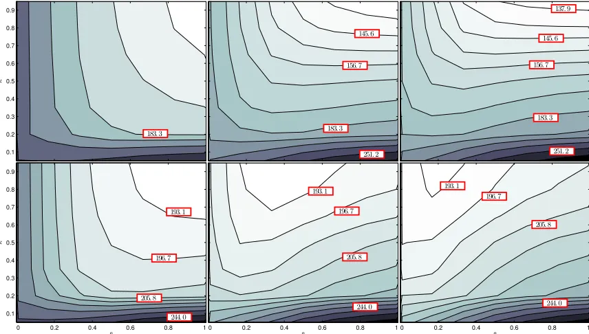
Figure 9: Train set (top) and test set (bottom) negative log-likelihood (perplexity) for the
Boltz-mann chain MRF with pseudo/full likelihood selection policy (PL1/FL). The x-axis,β,
corresponds to relative weight placed on FL and and the y-axis, λ, corresponds to the
probability of selecting FL. PL1 is selected with probability 1 and weight 1−β.
Con-tours and labels are fixed across columns. Results averaged over several cross-validation folds, that is, resampling both the train set and the PL1/FL policy. Columns from left to
right correspond to weaker regularization,σ2={500,2500,5000}. The best achievable
test set perplexity is about 190.
Unsurprisingly the test set perplexity dominates the train set perplexity at eachσ2
(col-umn). For a desired level of accuracy (contour) there exists a computationally favorable regularizer. Hence ˆθmsln acts as both a regularizer and mechanism for controlling accuracy and complexity.
pseudo likelihood is more traditional, for example, p(Y2|Y1,Y,3,X2)and p(Y2,Y3|Y1,Y,4,X2,X3)are valid 1st and 2nd order pseudo likelihood components.
We employ a subset of the features outlined in Sha and Pereira (2003) which proved competitive for the CoNLL-2000 shared task. Our feature vector was based on seven feature categories, resulting in a total of 273,571 binary features (i.e., ∑i fi(xt) =7). The feature categories consisted of word
140 150 160 170 180 190 200 210 220
neg. log−likelihood
0 0.2 0.4 0.6 0.8 1
190 195 200 205 210 215 220 225 230
β
neg. log−likelihood
0 0.2 0.4 0.6 0.8 1
β
0 0.2 0.4 0.6 0.8 1
β
Figure 10: Train set and test set perplexities for the Boltzmann chain MRF with PL1/FL selection
policy (see above layout description). The x-axis is againβand the y-axis perplexity.
Lighter shading indicates FL is selected with increasing frequency. Note that as the
regularizer is weakened the range in perplexity spanned by λincreases and the lower
bound decreases. This indicates that the approximating power of ˆθmsln increases when
unencumbered by the regularizer and highlights its secondary role as a regularizer.
the L2 regularizer, exp{−(2σ2)−1||θ||2
2}, which is strong whenσ2 is small and weak when σ2 is
large.
We demonstrate learning on two selection policies: pseudo/full likelihood (Figures 15 and 16) and 1st/2nd order pseudo likelihood (Figures 17 and 18). In both selection polices we note a
sig-nificant difference from the Boltzmann chain, βhas less impact on both train and test perplexity.
Intuitively, this seems reasonable as the component likelihood range and variance are constrained by the conditional nature of CRFs. Figure 19 demonstrates the empirical accuracy/complexity tradeoff
and Figure 20 depicts the effectiveness of theβheuristic. See captions for further comments.
8.4 Complexity/Regularization Win-Win
173. 0 λ 0.1 0.2 0.3 0.4 0.5 0.6 0.7 0.8 0.9 157. 9 173. 0 0.1 0.2 0.3 0.4 0.5 0.6 0.7 0.8 0.9 145. 2 150. 7 157. 9 173. 0 0.1 0.2 0.3 0.4 0.5 0.6 0.7 0.8 0.9 193. 3 198. 5 β λ
0 0.2 0.4 0.6 0.8 1
0.1 0.2 0.3 0.4 0.5 0.6 0.7 0.8 0.9 191. 0 193. 3 198. 5 β
0 0.2 0.4 0.6 0.8 1
0.1 0.2 0.3 0.4 0.5 0.6 0.7 0.8 0.9 191. 0 193. 3 198. 5 216. 9 β
0 0.2 0.4 0.6 0.8 1
0.1 0.2 0.3 0.4 0.5 0.6 0.7 0.8 0.9
Figure 11: Train set (top) and test set (bottom) perplexity for the Boltzmann chain MRF with 1st/2nd order pseudo likelihood selection policy (PL1/PL2). The x-axis corresponds to PL2 weight and the y-axis the probability of its selection. PL1 is selected with
probability 1 and weight 1−β. Columns from left to right correspond to σ2 =
{5000,10000,15000}. See Figure 9 for more details. The best achievable test set
per-plexity is about 189.5.
In comparing these results to PL1/FL, we note that the test set contours exhibit less
per-plexity for larger areas. In particular, perper-plexity is lower at smallerλvalues, meaning a
computational saving over PL1/FL at a given level of accuracy.
In Figure 5 we note this phenomenon when comparingσ2=1 toσ2=10 across the selection
policies PL1/FL and PL1/PL2. That is, the weaker regularization and more restrictive selection policy, that is, PL1/PL2, is able to achieve comparable test set perplexity.
For the text chunking experiments, we observe a striking win-win when using the Boltzmann chain MRF, Figures 9 and 11. Notice that as regularization is decreased (comparing from left to right), the contours are pulled closer to the x-axis. This means that we are achieving the same perplexity at reduced levels of computational complexity. The CRF however, only exhibits the win-win to a minor extent. We delve deeper into why this is might be the case in the following section.
8.5 λ,σ2Interplay
Throughout these experiments we fixed σ2 and either swept over (λ,β) or used the heuristic to
145 150 155 160 165 170 175 180 185
neg. log−likelihood
0 0.2 0.4 0.6 0.8 1
190 192 194 196 198 200 202 204 206
β
neg. log−likelihood
0 0.2 0.4 0.6 0.8 1
β
0 0.2 0.4 0.6 0.8 1
β
Figure 12: Train (top) and test (bottom) perplexities for the Boltzmann chain MRF with PL1/PL2 selection policy (x-axis:PL2 weight, y-axis:perplexity; see above and previous).
PL1/PL2 outperforms PL1/FL (Fig. 10) test perplexity despite PL1/FL including FL as a special case (i.e.,(λ,β) = (1,1)). We speculate that the regularizer’s indirect connection to the training samples precludes it from preventing certain types of overfitting. See Sec. 8.4 for more discussion.
how the optimal σ2 changes as a function ofλ. In Figure 21 we used theβheuristic to evaluate
train and test perplexity over a(λ,σ2)grid. We used CRFs and the text chunking task as outlined in Section 8.3.2.
For the PL1/FL policy, we observe that for small enoughλthe optimalσ2, that is, theσ2with
smallest test perplexity, has considerable range. At some point there are enough samples of the higher-order component to stabilize the choice of regularizer, noting that it is still weaker than the optimal full likelihood regularizer. Conversely, the PL1/PL2 regularizer has an essentially constant optimal regularizer which is relatively much weaker.
As a result, we believe that the lack of win-win for the chunking CRF follows from two effects.
In the case of the PL1/FL policy the contour plots are misleading since there is no single σ2that
performs well across allλ∈[0,1]. For the PL1/PL2 there is simply little change in regularization
necessary acrossλ.
9. Discussion
The proposed estimator family facilitates computationally efficient estimation in complex graphical
en-neg. log−likelihood
flops
140 160 180 200 220 240
2 2.01 2.02 2.03 2.04 2.05 2.06 2.07
x 1013
neg. log−likelihood
140 150 160 170 180 190
2.5 3 3.5 4 4.5
x 1013
Figure 13: Accuracy and complexity tradeoff for the Boltzmann chain MRF with PL1/FL (left) and PL1/PL2 (right) selection policies. Each point represents the negative log-likelihood (perplexity) and the number of flops required to evaluate the composite likelihood and its gradient under a particular instantiation of the selection policy. The shaded region is the convex hull of the points and represents empirically unobtainable combinations of computational complexity and accuracy. Particularly interesting is the difference between policies and against the discriminative CRF, cf. Figure 19.
ables the resolution of the complexity-accuracy tradeoff in a domain and problem specific manner. The framework is generally suited for Markov random fields, including conditional graphical mod-els and is theoretically motivated. When the model is prone to overfit, stochastically mixing lower order components with higher order ones acts as a regularizer and results in a win-win situation of improving test-set accuracy and reducing computational complexity at the same time.
It is interesting to note that the SCL framework may be generalized to random m-estimators beyond likelihood objects. That is, instead of a fixed m-function we may consider a linear combi-nation of stochastic objects (appearing or not with some probability). Such estimators go beyond traditional m-estimator but may be analyzed using techniques similar to the ones developed in this paper. Although not a random m-estimator, the work of Dillon et al. (2010) borrows SCL concepts to facilitate budgeted semi-supervised learning. This too would benefit from a random m-estimator interpretation and indeed many machine learning tasks may fit nicely into such a framework.