University of New Orleans University of New Orleans
ScholarWorks@UNO
ScholarWorks@UNO
University of New Orleans Theses and
Dissertations Dissertations and Theses
12-15-2006
Energy Efficient Cluster Head Selection in Fixed Wireless Sensor
Energy Efficient Cluster Head Selection in Fixed Wireless Sensor
Networks
Networks
Irfanuddin Ahmed
University of New Orleans
Follow this and additional works at: https://scholarworks.uno.edu/td
Recommended Citation Recommended Citation
Ahmed, Irfanuddin, "Energy Efficient Cluster Head Selection in Fixed Wireless Sensor Networks" (2006). University of New Orleans Theses and Dissertations. 476.
https://scholarworks.uno.edu/td/476
This Thesis is protected by copyright and/or related rights. It has been brought to you by ScholarWorks@UNO with permission from the rights-holder(s). You are free to use this Thesis in any way that is permitted by the copyright and related rights legislation that applies to your use. For other uses you need to obtain permission from the rights-holder(s) directly, unless additional rights are indicated by a Creative Commons license in the record and/or on the work itself.
Energy Efficient Cluster Head Selection in Fixed
Wireless Sensor Networks
A Thesis
Submitted to the Graduate Faculty
of the University of New Orleans
in partial fulfillment of the
requirements for the degree of
Master of Science
in
Computer Science
by
Irfanuddin Ahmed
B.C.A J.B. Institute of Technology, 2001
Acknowledgements
I would like to thank my advisor Dr. Jing Deng for his constant availability, guidance and
support. He is one of his classes encouraged me to take up research in Wireless Sensor Networks
for which I am very grateful to him. His clarity of thought and constant availability was a major
factor in this thesis. I would like to express my heartfelt appreciation for it.
I would also like to thank professors on my thesis committee Dr. Adlai DePano and Dr. Bin
Fu. I was honored to take classes under these distinguished professors, whose commitment and
knowledge about the subject helped me understand the intricacies of computer science. Learning
under them is a humbling experience. I express gratitude for getting an opportunity to learn
under them.
On a personal note, I would like to thank my family without whom; this would not have been
possible. It was their backing and resolve that helped me go through all the hurdles. I would also
like to take this opportunity to dedicate this thesis to my brother and my family who have been
there to back me whenever I needed them. Last but not the least I would like to thank Almighty
Table of Contents
Table of Figures ... iv
Table of Tables ... iv
Abstract ... v
Chapter I: Introduction... 1
I.1 Background ... 1
I.2 Energy Loss in CH Selection in Wireless Sensor Network...4
I.3 Thesis Organization……….7
Chapter II: Related Work... 8
Chapter III: Details of Cluster Head Selection Schemes... 11
III.1 Assumptions ... 11
III.2 Cluster Head Selection Techniques... 13
III.3 Cost & Overhead ... 18
Chapter IV: Performance Evaluation... 21
IV.1 Methodology... 21
IV.2 Network Types ... 22
IV.3 Network – Assumptions ... 23
IV.4 Results... 24
Chapter V: Conclusion... 36
Chapter VI: Future Work ... 37
References... 39
Table of Figures
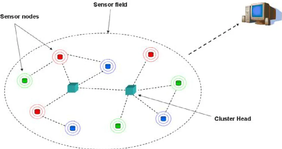
Figure 1: Wireless sensor network... 3
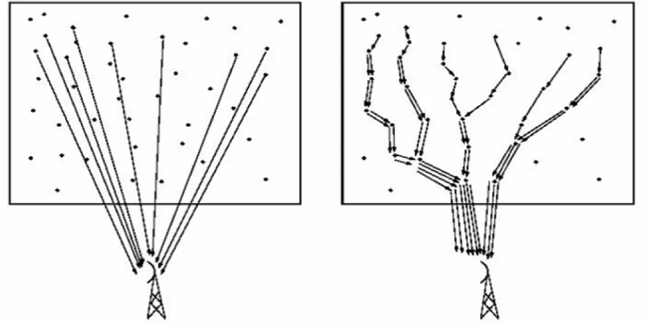
Figure 2: Single Hop Vs Multi Hop Network Topology... 5
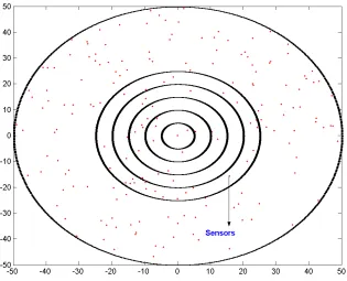
Figure 3: Distance Based Technique ... 15
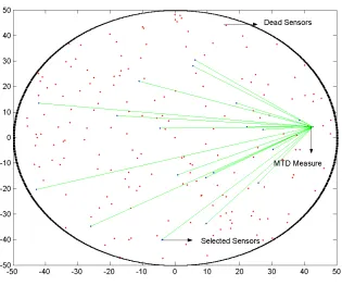
Figure 4: MTD Technique ... 16
Figure 5: Distance Node Degree (DNT) Technique... 18
Figure 6: Random Sensor Network for Cluster Radius 25... 25
Figure 7: Random Sensor Network for Cluster Radius 50... 25
Figure 8: Network lifetime – Random Network of Radius 25 ... 26
Figure 9: Network lifetime – Random Network of Radius 50 ... 26
Figure 10: Network lifetime – Random Network of Radius 100 ... 27
Figure 11: Custom network of radius 25 with condensed area ... 28
Figure 12: Custom network of radius 50 with condensed area ... 28
Figure 13: Network lifetime of CSN radius 25 with variable radii... 30
Figure 14: Network lifetime of CSN radius 50 with variable radii... 30
Figure 15: Cluster head selection plots in RSN... 32
Figure 16: Cluster head selection plots in CSN... 32
Figure 17: Lifetime-Coverage plot for custom network of radius 25 ... 33
Abstract
Energy is the main bottleneck for wireless sensor networks and it has dominating effects on
network lifetime. Sensors have finite energy and during the process of sensing and transmitting
data to the cluster head they lose energy. Sensors that are furthest away from the cluster head
require more energy than the closer ones. These losses of energy cause sensors to die faster,
lower coverage area and hence network death.
In this paper we investigate techniques to maximize the network lifetime by selecting the
most optimal cluster head. The proposed technique is in context of cluster-based wireless sensor
networks, the others being un-clustered sensor networks. The cluster head selection technique is
based upon distance and node degree. The key idea of the scheme is to choose new cluster heads
according to their distance and node degree toward the original cluster head location. The benefit
of such a technique is to reduce the overall consumption of energy, thus increasing the network
I Introduction:
I.1 Background:
Recent technological advances have led to the development of smaller, cheaper,
multifunctional and efficient sensors. Sensors are small radio devices which are deployed to
relay sensed information. Sensors are made up of a radio, a processing unit, memory unit,
sensing unit and an energy source which is usually a battery. Sensors along with base station
together form one sensor network.
Unlike the traditional sensors, in the remote sensor network a vast numbers of sensors are
densely deployed. Multitudes of sensors are deployed in remote inhospitable environments to
better study and understand it. These sensors network and transmit sensed data over a wireless
channel.
When their sensed data is intelligently combined it gives us a better understanding of the
remote environment. Such application of sensors can be seen in areas of defense, human
sciences, geology, biological contamination, etc. All these areas are considered inhospitable yet
information about the extent of their impact is essential in critical decision making. Since sensors
operate in these inhospitable environments, they need to be robust, reliable, and efficient with
high lifetime. These factors are essential to gather data of better quality and for longer length of
time.
In order to study phenomenon sensors can be deployed in the following ways.
Firstly, sensors can be in remote location far away from the phenomenon. Sensors like these
Secondly, sensors can de deployed in numbers in and around the phenomenon. The topology
of the network need not be pre-determined. They can be dropped in numbers in and around the
phenomenon. But this kind of deployment requires the sensors to have self-organizing
capabilities using intelligent algorithms and protocols.
These sensors do not just relay raw data. The sensed data is partially processed using an
on-board processor and is usually compressed. This compression helps the sensors to reduce the
energy required to send the data. In this way it can send more data for a given amount of energy.
The compressed data is then relayed forward to central nodes where it is further processed.
The feature described above of a sensor network has wide applications. Some of them include
but are not limited to military, health, wildlife habitat monitoring, structural monitoring, target
tracking etc. In essence, sensor networks provide immediate and fast access to partially
processed end-user data.
In the future, we envision development of better sensors like “smart dust” along with
algorithms and protocols. Sensor networks will become part of our day-to-day lives. Variety of
applications can be envisioned that depend upon the wireless ad hoc networking technology.
Since the requirements of sensor networks are so unique than the techniques proposed for
traditional wireless ad-hoc networks may not be well-suited for sensor networks.
The points below illustrate this further
The number of sensors deployed in a network is exponentially higher to number of nodes
in ad hoc network;
Sensor nodes are less mobile;
Sensors are densely deployed to overcome fault tolerance and energy constraints;
Ad hoc networks usually use point-to-point communication while sensors use broadcast
methods to communicate;
Since sensors are deployed in high numbers, they may not have a unique global ID for
unique identification. A unique global ID also increases length of data packet;
Sensors are constrained in memory, energy and processing capabilities;
Sensor location is not predetermined.
There are different kinds of sensors depending upon the physical variable they measure.
These variables can be thermal, electromagnetic, mechanical, optic and radiation, acoustic,
motion, orientation and distance sensors. They are able to monitor different variables like
temperature, heat, pressure, chemicals, light, radiation, sound etc.
Micro-sensing and wireless networking, together form the sensor network. Their application
in day-to-day life can be seen extensively in video surveillance, robotics, automotives, air traffic
One of the most important constraints of a sensor network is energy. Energy is usually
supplied by a local battery. Since sensor nodes are deployed in hostile environments it may be
hard or impossible to replace or recharge the battery. Thus protocols need to be energy-efficient
to best conserve and retain the sensor while still maintaining the data quality. Trade-offs can be
made with other factors depending upon the priority, quality and nature of sensed data.
In this work we focus on methods and techniques to preserve and efficiently use energy in a
sensor.
I.2 Energy Loss in CH Selection in Wireless Sensor Network:
Many researchers are currently involved in the development of energy-efficient schemes for
wireless sensor networks. Most of the latest studies mainly focus on different algorithms,
transmission, routing protocols and data compression techniques to save battery and extend the
lifetime of the sensor and the network.
Sensors are usually classified into different types of networks depending upon topology, order
of data traversal, routing methods etc. Some of them are explained below.
They can be classified as clustered or un-clustered. In the case of without clusters, sensed data
can be relayed in a single hop or multi-hop fashion to the base station or data sink. In
cluster-based sensor networks, sensors can relay their sensed data to the appointed or elected cluster
head of a given cluster. Data to the cluster heads can be transmitted in a single and multi-hop
fashion.
Cluster heads can be special kind of sensors with higher energy, processing or memory. In
serves as cluster head in a given round or it can elected by sensors in the cluster itself. This is
also called “heterogeneous sensor network”.
Custer heads can be ordinary sensors given additional duty of a cluster head due to various
selection parameters which can be distance, energy, centrality, etc, elected either by base station
or sensors in the cluster itself. This is also called “homogeneous sensor network”.
Sensors in cluster-based sensor network can be of fixed or dynamic nature. Fixed cluster
sensor network is composed of sensors that are associated with a single cluster permanently from
the moment they are deployed till the time they run out of energy. Dynamic cluster based sensor
network, the sensors change their cluster depending on the parameter on which it is pre
programmed. Some of the parameters can be distance, energy, proximity to the data sink, size of
the cluster etc.
In our work we look into the case of fixed cluster-based single-hop sensor network. In
particular we examine the loss of energy incurred by them due to different selection techniques
of the cluster heads. In fixed cluster-based sensor network, sensor nodes are dispersed over the
area of the cluster.
Intuitively, we know that as the distance between sensor and cluster head increases, the
transmission energy of the sensor increases. With the traffic pattern and energy consumption rate
the distribution of sensors with higher energy constantly changes in the cluster.
To compensate for this constant change we need to co-locate the cluster head so as to
minimize the energy consumption of sensor thus increasing the network lifetime. This process of
co-locating involves the process of identifying potential sensors that can serve as cluster heads,
and selecting one among them.
The important point is: which parameters need to be considered for selection of cluster head.
As we shall discuss further on we will observe that certain parameters have profound impact on
the selection of cluster head.
Since network lifetime is tightly coupled with the lifetime of sensors. It is essential that we
look for methods to first increase the lifetime of sensors. This, in turn, will have a direct impact
on the lifetime of the network.
There can be many factors that help in cluster head selection. But we have to keep in mind
which factors consume more energy. In order to determine certain factors, the sensor needs to
spend energy. For instance in measuring the distance between sensor A and sensor B, if A is
measuring the distance between itself and B, then it spends energy proportional to the distance
between itself and B. Hence, we have to make sure that the chosen factors are energy-efficient
It is important that sensors select a cluster head autonomously instead of transmitting the
selection parameters to the base station. This is important because of two important factors. First,
it saves energy of transmission to the base station. Secondly, it saves time of transmission,
selection and retransmission of results. This helps the sensors get back to sensing faster and in an
energy-efficient manner.
In this work, we propose a technique to select a cluster head autonomously and in an energy
efficient manner. This mitigates the adverse impact of base station cluster head selection on the
network lifetime. The technique takes into consideration the then present traffic pattern and
sensors above the minimum energy threshold and then calculates the best sensors from the list of
available ones to select a new cluster head.
This work, also demonstrates the performance gain in selection of cluster heads from the
proposed technique. The technique is deployed in generic sensor network and real life networks.
The generic sensor network simulates a standard sensor network deployed over an area
randomly. While the real life network tries to simulate disproportionate distribution of sensors
which can be expected in real life environments.
The results show that the proposed technique does enhance the lifetime of the sensor and also
the lifetime of the network.
I.3 Thesis Organization:
The remainder of this thesis is structured as follows: In Chapter II, we review the related
work, what has been proposed in a matter of efficient cluster head selection techniques and
extending the network lifetime in general. We present our technique and discussions in Chapter
Distance Node-Degree Technique (DNT) achieves when compared to other schemes. In Chapter
V, we summarize the work. Finally, Chapter VI proposes ideas, possible future research related
to our scheme.
II Related Work:
Sensor networks have evolved as an important platform for research and computing. The
application of these networks in areas of military, medicine, surveillance, day-to-day activities
has increased considerably. It is due to this fact that increasing research is being conducted on
these specialized devices and networks. These tiny sensors carry along with them sensing unit,
processing unit, memory unit, mobility unit if any and a energy source that is battery. It is under
very rare circumstances that the sensors battery is manually replaced or recharged, due to the
nature of their deployment. Hence energy is the most telling factor in a sensor.
Energy efficiency is the most researched topic in wireless sensor networks. Over the years
many interesting studies have been proposed to reduce the energy consumption of the sensors
and increase the lifetime of the network.
Many papers like [1, 2, 3, 4, 7, 11, 16] discuss the different techniques in which energy
efficiency can be attained. Sensors once deployed on the field, either need to be clustered or left
un-clustered. Most of the techniques discuss about clustering of senor networks after their
deployment. There are only a few papers that directly deal with the cluster head selection in a
cluster like HEED, Fuzzy Logic, LEACH-Centralized, LEACH.
The reason for the optimization of the cluster head selection techniques is to reduce energy
consumption. There are many parameters that help make this decision. Different technique uses
placed in inhospitable environments with a non pre determined topology. We argue that this is
one of the prime reasons for autonomous cluster head selection and also an energy efficient one.
Nonetheless, we will observe schemes that require sensors to transmit cluster head selection
information to the base station for processing. This is not only costly but also inadvertently
reduces the network lifetime.
The HEED [1] protocol initially distributes the sensors in different clusters using a distributed
clustering algorithm. For intra cluster energy efficiency it uses energy consumption as a
parameter to decide the cluster head The energy consumption is determined by the average
energy it takes for a sensor to transmit a unit of data to the cluster head. It uses Average
Minimum Reachability Power (AMRP). For every given sensor which can be potential cluster
head AMRP is calculated. The AMRP of a sensor is the measure of the expected intra cluster
communication energy consumption if the given sensor becomes a cluster head. HEED assumes
variable power levels are allowed in intra cluster communication.
The LEACH [4] protocol uses a deterministic cluster head selection technique. LEACH uses
randomized rotation of high energy cluster head positions among the sensors in the network. In
this way load of the energy consumption is distributed among other nodes.
The operation of LEACH is divided into rounds. Each round has two phases setup phase and
steady phase. In the setup phase sensors are organized into clusters. In the steady phase, data
transmission from the sensors to their respective cluster head begins. Since being cluster head is
an energy consuming process each node takes turn to become cluster head.
Each sensor elects itself as cluster head in the beginning by assigning itself a probabilistic
value. This value is based on energy of the node, recently performed cluster head operation or
probabilistic value and sensors with lower energy have lower value. The value also get effected
due to other factors too. If the sensor was earlier a cluster head in the same round then the value
goes down when compared to a sensor with similar energy and which has not served as cluster
head. The LEACH scheme tries to balance the energy consumption of the sensor by rotating the
duties of cluster head for a given list of sensors. This enables the sensors to serve as cluster head
but also not sap their energy to below critical threshold. Thus the sensor with the higher value
becomes the cluster head for a given round.
The scheme in paper [16] describes energy adaptive method to select cluster heads. The main
idea is to avoid choosing sensor with lower residual energy and higher energy dissipation as
cluster heads. It bases its selection on three factors: initial energy level, total dissipated energy
level of the sensor and initial average energy level of all in-cluster sensors.
In this method, the node after determining it current residual energy level checks with the
current average energy level. The current average energy level is determined by taking the
average of the current residual energies of nodes in the cluster. If it is lower then; it lowers it
probability of becoming the next cluster head, else it will increase it.
LEACH-Centralized [7] uses a centralized clustering algorithm to form clusters and associate
cluster heads for the sensors. First the sensors send their location information to the base station.
Then the base station computes the average node energy and nodes which are below the average
cannot be cluster head for the given round.
Using the remaining nodes as possible cluster heads, the base station finds cluster using the
simulated annealing algorithm [5].
This algorithm tries to minimize the amount of energy for the non cluster head sensors to
cluster head and the non cluster head nodes. The algorithm allows the sensors to disassociate
themselves from earlier cluster head and scan the area for other cluster heads. If a sensor finds a
cluster head closer to it, than the others it associates with the closer one. This process of dynamic
association enables the sensor to make a decision in its best interest, by utilizing the least power
to communicate with the cluster heads.
Paper [3] proposes a fuzzy logic approach to cluster head selection. The sensor is selected by
the base station after sensors transmit the selection parameters to it. The selection parameters are
node concentration, current residual energy, node centrality with respect to entire cluster. These
parameters are also refereed as fuzzy descriptors. This technique uses a central control algorithm
to select the cluster head. The model of fuzzy logic control consists of fuzzifier, fuzzy rules,
fuzzy inference engine and a defuzzifier. It uses the most commonly used fuzzy inference engine
called Mamdani Method [6]. The process is performed is four steps: Fuzzification of input
variables, rule evaluation, aggregation of rule outputs and defuzzification.
The method described above relies on a complex computing structure to process the selection
parameters to output the best probability of a sensor acting as the next cluster. This method
requires heavy processing, memory and energy, which is not feasible for our sensor network.
III Details of Cluster Head Selection Schemes:
III.1 Assumptions:
Sensor networks differ in protocols, data sensing pattern, density, coverage and topology
depending on the nature of data they are sensing or quality level of data that needs to be
We make certain assumptions for the network that we studied, which are as follows:
●Density of the network can increase exponentially to gather better quality data. This
increase is due to limited sensing range of the senor for low energy consumption in order to
have better coverage; we need to have more sensors. Hence the increase. We in our work use
between 0.01 to 0.05 sensors per unit area.
●Sensors transmit the data to the cluster head in a single hop fashion.
●Sensors constantly sense important data and relay it to the cluster head. They relay it at a
constant rate of one packet per time unit.
●Sensors do not have mobility in the field.
●The cluster head receives the sensed data from other sensors, and periodically send a
control signal across the cluster.
●The first cluster head after deployment is in the center of a given cluster. Initially all the
sensed data is sent to the first cluster head.
●The cluster head selection schemes start after the initial cluster head drops below the
minimum energy threshold.
●The network is considered dead if it falls below a pre determined sensing coverage area
called minimum coverage threshold.
●Sensor network is made up nodes that are similar to each other is every aspect. This
III.2 Cluster Head Selection Techniques:
III.2.1 Motivation:
Sensors once deployed are divided into clusters. Each cluster has a cluster head and a certain
set of sensors assigned to it. This process of dividing the sensors into clusters is called
“clustering” and is usually performed by a clustering algorithm. This initialization process also
called the “setup phase” is usually done by the base station or other method as determined by the
protocol.
The next phase is the steady phase. It is in this phase that the sensors assigned to a cluster
transmit the sensed data to the cluster head. The transmission is either single hop or multi hop.
The cluster head in turn can either transmit it forward to the base station directly or to other
cluster heads depending upon the agreed protocol. After a period of time transmitting data by
sensors to the cluster head within the cluster, the sensors start losing energy and hence go below
an energy threshold, below which the sensor is considered dead.
Due to different traffic rate, congestion, presence of data to be sensed and distance between
sensor and the cluster head; different sensor have different energy consumption rate. Due to this
uneven energy consumption rate the topology of the network changes constantly.
Having a cluster head in a predetermined position with a changing network topology, leads to
low network lifetime. The location of the cluster head or the sensor holding the duties of the
cluster head should also change. The change should hence increase the sensor lifetime and also
III.2.2 Methodology of Proposed Schemes:
We examine a single cluster and the methods used to select cluster heads. The cluster can be
part of a bigger sensor network with multiple clusters and remote base station. When the first
cluster head (i.e., the one in the middle of the cluster) drops below the minimum energy
threshold we begin the process of selecting the new cluster head. Minimum energy threshold is a
pre determined constant value, if a sensors residual energy drops below this value it is considered
dead.
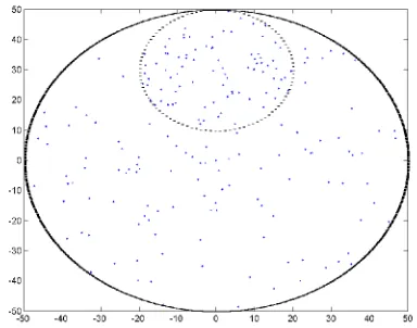
III.2.2.1 Distance-Based Scheme:
During the steady phase, in the distance-based scheme, the cluster head of the earlier round
scans the area around it for a radius equal to node-sensing range. If no sensors above the
minimum energy threshold are found then the radius is doubled, then tripled and so on and so
forth.
This process goes on until at least one sensor is located in the vicinity. The sensor which is the
closest to the earlier cluster head is elected as next cluster head. This selection process of sensors
carries on until the coverage area drops below a minimum coverage threshold.
This scheme works well in clusters with high node density and with normal sensor
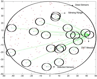
Fig. 3 Distance Based Selection method
The above figure is a sample of a random sensor network of radius 50 with 0.02 node density
per unit area. The circles highlight the increasing radius of scanning if no sensors are located
with energy more than minimum threshold. The innermost circle is reflective of the node range
of the sensor, and the increase of it in multiples.
III.2.2.2 Minimum Total Distance Scheme:
In this scheme the cluster head of the earlier round scans the whole cluster for sensors with
energy higher than minimum threshold. Once the sensors are located, a measurement of
Each sensor is assumed to the next cluster head and sum of distances between itself and the
rest of the selected sensors is measured. The sensor with the least value of this summation of
distance is selected as the next cluster head.
This is intuitively the best selection method but it is very costly. The amount of energy spent
by each sensor in calculating the distance between itself and other sensors is very high. In an
energy-conscious networking environment like the wireless sensor network, this kind of energy
usage is not acceptable. This technique, although good, is costly and would suit base station
processing.
Fig. 4 Minimum Total Distance Technique
The above figure is a sample of Minimum Total Distance technique cluster head selection
distance to other active sensors. This figure is reflective of a sensor going through that process.
The sensor measures its distance to all other sensors (the green lines). As we can see this clearly
is an energy-sapping process.
Hence, even though this is intuitively a better technique, it is not energy-efficient. Far too
much energy is expended during the selection process.
III.2.2.3 Distance-Node Degree Technique (DNT):
As we have seen earlier schemes are either too costly (energy consumption) or they do not
provide us with better cluster heads for the network. So in order to provide better selection with
less energy consumption we proposed a new technique called Distance-Node Degree technique
(DNT).
In this method the cluster head of the earlier round scans the cluster for sensors above the
minimum energy threshold. The selected list of sensors is applied with a cost function.
)) ND * (Q2 (D min
Pi i i
In this function Di is the Distance between the sensor and the original cluster head (i.e., the
first cluster head after network deployment)
NDi is the node degree of the sensor, which is calculated as follows: the sensor scans the area
within the node sensing range. For every sensor that is above the minimum energy threshold the
sensor adds one in the node degree.
Q2 is a constant called the node degree constant.
The sensor which has the least value of the above cost function is selected as the next cluster
As we will observe later the value of Q2 is very essential to the selection of best cluster head. It
balances the weight given to both distance and node degree of a sensor.
This scheme described an energy efficient and autonomous selection method. This scheme
will enable the sensors to make autonomous cluster head selection decisions without involving
the base station. This has two potential benefits, the reduced cost of transmitting the selection
parameters to the base station and the time delay between selection need and selection decision.
Fig. 5 DNT Technique
III.3 Cost & Overhead:
We will initially look into the different cost factors. Then we will look individually in each
During the lifetime of the sensor the activities it performs are: sensing data, processing data,
transmitting data, receiving data. In our network we assume that only transmitting data requires
considerable energy, while the others use negligible amounts.
The energy required to transmit data depends upon the size of data and distance it has to be
sent. For simplicity we assume the size of the data is unity. Then the energy to transmit becomes
directly proportional to the distance between itself and destination. Let us look into each of the
proposed schemes and cost or overhead they incur during selection of new cluster head.
The sensor energy consumption is calculated using the following equation. This equation is
derived from paper [17].
K2
γ
D)^ ,
λ.K1.max(D
Ei min
Where Ei is the energy consumption for senor i, is the sensor traffic rate, K1 is the energy
consumption rate constant that is related to distance, represent the path loss exponent (usually
>= 2), Dmin is the minimum distance below which the energy consumed by the sensor is
constant, D is the distance between sensor and the cluster head, K2 is the data receiving constant.
For simplicity we assume Dmin to be zero.
Distance Based Scheme: This scheme consumes the least energy while selecting a new
cluster head. The process of selection consists of scanning the sensing range near the earlier
cluster head.
The sensing range is usually a small value. The energy to scan the area can be derived from
the above equation, in which “nodeRange” is equal to the sensing range of the sensor.
K2 γ) ^ (nodeRange * K1 * λ
E
Minimum Total Distance Scheme: This is intuitively the best scheme for selection of
cluster heads. But in terms of energy used it is costly. The energy used by this scheme can again
be derived from the following equation.
min(Di) MTD )^2) y (y )^2 x (x D p i 1 i i p n 1 n i n i n i
Here p is the list of sensors in the cluster that have more than the minimum energy threshold,
Di is the summation of distance between the sensor “i” and the other sensors, MTDi gives the
minimum distance. Sensors with this distance as the total distance become the next cluster head.
Even though this scheme does provide us with an intuitively better selection it is too costly to
implement in energy conscious sensor network. As we can clearly see the amount of energy used
to calculate the distance between a given sensor and others is very high.
We will see further in the simulations the effect of such a costly scheme on the network
lifetime.
Distance-Node Degree Scheme: The cost of this scheme is just a little bit above the distance
based scheme but the performance is better. In this scheme the earlier cluster head scans the
cluster for potential sensors using these conditions: sensors should have more than the minimum
energy threshold, sensors should not have served as cluster heads earlier.
In this process their is certain amount of energy spent which can be calculated as follows
K2 γ )^ D (R * K1 * λ
Ei Org.CH
Here “i” is the cluster head of the earlier round, R is the radius of the cluster and Dorg.CH is the
cluster when the network is deployed. As we can see this is a done only once during a round of
cluster head selection.
IV Performance Evaluation:
IV.1 Methodology:
In order to implement our cluster head selection techniques, we first need to simulate a close
to real time, sensor network. We first study the types of sensors networks, their classification and
then model our network to simulate these real time networks.
These simulations of networks help us to determine the best cluster head selection scheme for
different types of network.
A standard energy consumption model is needed to determine the energy consumption rate of
each sensor for every data transmission.
Energy consumption for unit data packet for a sensor is given by the following:
K2 γ D)^ , max(D * K1 * λ E )^2 y -(y )^2 x -(x D min i q i q i i
In order to determine this, we first need to calculate the distance between the sensor and the
receiver. This energy consumption rate is the amount of energy deducted from the sensors
energy reserves.
If a sensor A transmits N data packets to sensor B; the energy consumption rate for the data
Sensors also consume energy when they receive data packets. This energy is quantitatively
very small compared to the transmission energy. This is the reason we do not consider this
energy.
This energy consumption model is implemented for the variety of sensors networks we
simulate.
IV.2 Network Types:
In our study we mostly use different kinds of 2-D networks. Each one of those network
convey a different state of the sensing environment. Each of them is also used for different
sensing purposes. The networks are: Random Distribution Sensor Network, Custom Distribution
Sensor Network.
Random Distribution Sensor Network: The topology of this network is the even
distribution of sensors across the cluster. This gives the network the maximum coverage area.
They are usually deployed in situation where the phenomenon is evenly spread out, where all
regions of the phenomenon need to equally sensed. The deployment of such network resembles a
manually planted sensor network.
Custom Distribution Sensor Network: The topology of such networks more or less
resembles real life situations. The sensors when dropped from a height or deployed scatter across
the floor in an uneven fashion. This resembles sensors being dropped for surveillance from a
plane etc. Sensors when deployed on a geographically uneven terrain, causes uneven
distribution. This leads to pockets in the cluster, with certain areas of high concentration and
certain scanty areas. These are the kind of networks we are most interested in primarily because
IV.3 Network - Assumptions: Both our sensor networks are designed as follows:
Network is made up of high number of nodes. Cluster density varying between
densities 0.01-0.05.
Cluster of different radii are also simulated. Radii from 5-20 times the node sensing
range are used.
We consider the network dead when the coverage area drops below “40%”. This
number was derived from [18] which consider this number as “high collapse risk level”
when more than one third of the sensors have used their energy resources.
Data transmission from nodes to the cluster head is carried out in a single hop
fashion.
Nodes in the network do not have a sleeping mechanism build in.
All nodes have an initial battery energy level of 10^5.
The path loss constant is set to 2 for our entire simulations both custom and
random.
Amount of energy used by nodes to sense within the sensing range is negligible.
In custom sensor network we use area called “condensed area”. This area has 2.5
times more node density than other areas. This area reflects a situation, where sensors are
unevenly distributed and hence higher concentration.
All nodes in the network are immobile. They retain the same location after being
deployed and are location aware.
The first cluster head called the “original cluster head” of the network is the sensor at
the middle of the cluster. In our 2-D network the co-ordinates sensor at (0,0) forms our
The node sensing range is set to 5. This value is used so that the technique can also
be implemented for networks with small cluster radii.
The cluster head periodically broadcasts control signal over the cluster, for the
sensors to transmit it the sensed data.
IV.4 Results:
All our simulations have been run on Matlab 7.0.1, and our data set consists of 100 different
network topologies for each of the networks generated by our program.
IV.4.1 Random Sensor Network:
We simulate four techniques on a random sensor network. They are: Minimum Total
Distance, Average Minimum Reach ability Power (AMRP) from HEED protocol, Distance
Based technique (DT) and Distance-Node degree technique also called “DNT Scheme”.
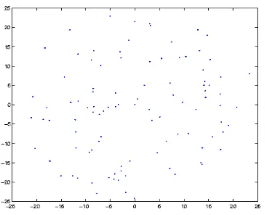
The simulations were run for 100 different network topologies of the similar nature. Below
we visually represent how a typical random sensor network appears. Fig. 6 illustrates the random
sensor network for a cluster of radius 25. Similarly Fig. 7 illustrates random sensor network for a
Fig. 6 Sample Random Sensor Distribution over Cluster Radius 25
Fig.7 Sample Random Sensor Distribution over Cluster Radius 50.
As we see from the above figures the networks are of similar nature distributed over different
cluster areas and different node density.
Further we illustrate the network lifetimes of the different techniques in this family of random
networks.
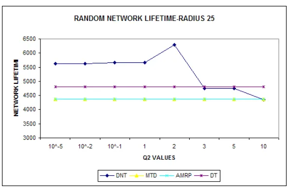
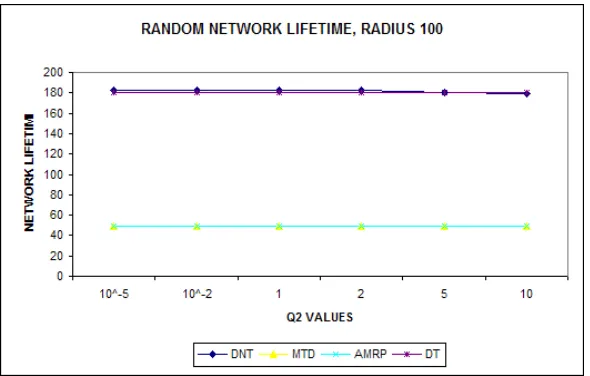
Figures 8, 9, 10 shows the average network lifetime observed for cluster of radii 25, 50, and
100. We have taken an average of 100 such network topologies with similar nodal density and
cluster radius for each graph.
Our objective in the plots was to show the behavior of a given network when the value of Q2
changes. As we observe in almost all the plots when Q2 value is 2 the DNT scheme outperforms
the other schemes. This value of “2” was arrived at after exhaustive simulation performed on
hundreds of network topologies of similar nature, size and density.
The definition of network lifetime in our simulation is the total cumulative lifetime of all the
cluster heads that served during the lifetime of the network.
We define lifetime in this fashion due to our traffic pattern. We assume that all our nodes are
sensors are supposed to transmit the data to the cluster energy till the cluster head runs out of
energy. We take the lifetime of the cluster head as a measurement factor.
Fig.8 Avg. Network Lifetime for MTD, AMRP, DT, DNT schemes over Cluster Radius 25
Fig. 10 Avg. Network Lifetime for MTD, AMRP, DT, DNT schemes over Cluster Radius 100
Fig. 8,9,10 Network Lifetimes measured in a Random network using Minimum Total Distance
(MTD), Average Minimum Reach ability Power(AMRP), Distance Based Technique (DT),
Distance-Node Degree Technique (DNT).
The network lifetime of the Distance-Node degree technique is slightly higher than distance
technique. As the value of “Q2” increases, the distance node degree scheme given more weight
to sensors with higher number of active neighbors. This is reflected in the lifetime of the sensor
network. When the value of “Q2” increases further, the probability of selecting sensors with
high number of active neighbors increases.
This leads to the DNT scheme giving less weight to the distance, which causes it to move
away from the center. As we saw from the distribution of sensors in the random network, the
sensors are almost evenly distributed. Therefore, when the DNT scheme gives less weight to the
distance between selected cluster head and distance to the original cluster head; it leads to the
We know from our energy consumption equation that as distance between sensors increase
the energy dissipated also increases. Due to this we observe the drop in the network lifetime for
DNT schemes with high “Q2” values.
IV. 4.2 Custom Sensor Network:
We deploy the same techniques as discussed above on a custom network of varying
condensed area size. In these simulations we use custom networks of radii 25, 50, 100. Each of
these clusters is tested with condensed area of 1/10, 1/5,1/2.5, 1/2 times the cluster radius.
These condensed areas have 2.5 times the node density as compared to other areas. Following
figure will provide a visual illustration of the custom network. Fig. 11, 12 has cluster of radius
25, 50. Each of them has a condensed area radius 1/2.5 times the radius of the cluster.
Fig. 11 Cluster Radius 25, Condensed Area 2.5 times
node density
Fig. 12 Cluster Radius 50, Condensed Area 2.5 times
node density.
Further we illustrate the network lifetimes observed with the schemes on these networks. As
as the value of Q2 increases the cost function discussed earlier gives more weight to the node
degree of a sensor as a criteria for selection.
If the value is increased unchecked then the selection becomes node degree centric. This will
lower the lifetime of the network because sensors with higher node degree are selected as cluster
heads and the distance is not taken into consideration.
Extensive simulation results again show that when Q2 equals 2. The DNT technique out
performs the other schemes.
Figures 13, 14 are plots of technique implemented on custom network with variable
condensed area radius.
Fig. 13 (a) Condensed Area of Radius 2.5 Fig. 14 (a) Condensed Area of Radius 5
Fig. 13 (c) Condensed Area of Radius 10 Fig. 14 (c) Condensed Area of Radius 20
Fig. 13 (d) Condensed Area of Radius 12.5 Fig. 14 (d) Condensed Area of Radius 25
Let us observe the simulation results plots here. From the above figures we see a significant
increase in lifetime of the custom sensor network. We observe again, that as the value of “Q2”
increases the selection of DNT scheme becomes node centric. But we also know that these
networks are special where the node concentration in certain pockets of the cluster is higher than
the others. Due to this we observe a little difference in performance of this network from the
random sensor network for higher “Q2” values.
Extensive simulation has shown us that when Q2 is equal to 2 the network lifetime is higher.
But is also shows us that, in certain network topologies of custom network of similar
concentration of nodes, the higher Q2 value performs even better than Q2 equal to 2. But these
Since these occurrences do not form a bulk of the simulation, we still select Q2 equal 2 as the
safe bet for higher network lifetime.
IV 4.3 Cluster Head Selection Plots:
In the plots below we take up a random and custom network and plot the sensors selected as
Cluster heads in each of the schemes individually.
This will visually illustrate the pattern of selection of cluster heads in each of the schemes and
differences between them. Fig. 15, 16 shows us the different sensors elected as cluster heads.
RANDOM CH PLOT CUSTOM CH PLOT
Fig. 15 (a)Random Network- MTD CH Plot Fig. 16 (a) Custom Network -MTD CH Plot
Fig. 15 (c) Random Network- Distance Only CH
Plot Fig. 16 (c) Custom Network Distance Only CH Plot
Fig. 15 (d) Random Network -DNT CH Plot Fig. 16 (d) Custom Network - DNT CH Plot
Fig. 15 Sensors Plots for Random Distribution network. Red color on the plot show the sensors selected as CH and the numbers signify the order in which they were selected
Fig. 16 Sensors Plots for Custom Distribution network. Red color on the plot show the sensors selected as CH and the numbers signify the order in which they were selected
Let us study the above figures here; the MTD scheme in both the network selects the sensors
with least cumulative distance. As expected those sensors have to one closer to the center.
Therefore we observe a similar pattern of selection in both types of networks.
Fig. 15 (b), 16(b) represents the Average Minimum Reach ability Power scheme from the HEED
protocol. AMRP relies on the minimum energy consumption rate of sensor for cluster head
selection. Energy in turn relies on distance to determine the consumption rate. Hence the selected
Fig 15(c), 16(c) illustrates the distance technique as we can clearly see the sensors are closer to
the center purely on node availability and distance basis.
Figures 15(d), 16(d) visually appears as hybrid between MTD, AMRP and Distance Technique.
The energy consumption of the scheme is also hybrid in nature consuming slightly greater than
distance technique but far less AMRP or MTD techniques.
IV 4.4 Lifetime-Coverage Plot:
Lifetime coverage plot shows us the behavior of a scheme in its lifetime. The definition of
lifetime in this plot is the time from which the sensors start transmitting the data to the cluster
head till the time the network coverage area falls below 40%.
The plots below are for custom sensor network. We try to study distance node degree lifetime
(Q2=2) along with other schemes. This plot gives us an insight into the behavior of coverage
area throughout the lifetime of the network.
Fig. 18 Lifetime Coverage for cluster of radius 50,with condensed radius 20 with 2.5 times the node density
In the above figures we illustrate the different techniques and the best case for DNT technique
(i.e. Q2 =2). The figure illustrates that DNT technique works better than others by selecting the
best cluster heads consistently in custom sensor network.
Similarly we also plot the lifetime coverage chart Random Sensor network and we observe
that even though the lifetime of the DNT technique is higher than other including Distance based
technique; In its lifetime it consistently performs over and equal to the distance technique.
The definition of coverage area is an amount of area of a cluster that can still be sensed. The
area can only be sensed by sensors which have energy above the minimum threshold. The total
coverage area is sum of the individual areas covered by sensors. If this total coverage area falls
Fig. 19 Lifetime Coverage for cluster of radius 50 in Random Network
Fig. 20 Lifetime Coverage for cluster of radius 50 in Random Network.
As we observe the performance of DNT technique even though is higher in the best case
scenario. Over the period of the network lifetime it performs closer to the distance based
This shows us that DNT scheme is better suited for custom networks which are a simulation
of real world sensor networks.
V Conclusion:
We have proposed a distance-node degree based technique to extend the lifetime of the
network.
The distance-node degree technique acquires a balance between the cost-efficient distance
technique and the very costly but intuitively better minimum-total-distance technique. DNT
technique utilizes the distance of the selected sensor and the node degree of the sensor in a cost
function with a constant Q2. The balanced selection of Q2 enables the scheme to select sensors
which are the best suited for the responsibility given a certain condition of the network which
leads the DNT scheme to perform much better than the others.
Through extensive simulation, we have shown that our proposed scheme extends the lifetime
of the network. We have also shown that the scheme is energy-efficient in terms of selection of
cluster head and also enables the sensors to make autonomous decisions.
In the best case scenario, we have seen the DNT scheme having a higher coverage area than
the other scheme throughout the lifetime of the network.
Our scheme also does not rely on the base station to make selection decisions. This capability
to make autonomous decisions enables the sensor network to consume less network and energy
resources. This inadvertently enhances quality of data received by reducing the traffic on the
wireless channels, reducing collisions of data, which in turn reduces retransmissions.
Finally, the efficiency of the scheme is illustrated when comparing with the mentioned
VI Future Work:
Through our simulation we have tried to mimic the real-world situation. Nonetheless, the
width and depth of wireless sensor networks is humongous which leaves more than enough
opportunity for better schemes to be developed.
The huge amount of parameters involved in a wireless sensor network like routing, data
transmission, clustering, cluster head selection, sleep scheduling etc. All these when embedded
with the proposed scheme with further enhance the network lifetime.
In our work we simulated with an initial cluster head in the middle of the cluster. Future work
can decide on deployment while the base station is still collecting data about the sensors to select
the best fit sensor as cluster head and not use a pre determined cluster head.
Many sleep scheduling schemes can also be implement along with DNT scheme to further
enhance the network lifetime.
The scheme proposed in this paper is a reactive scheme. By this we mean that after the
network deployment the scheme waits for the earlier cluster head to drop below its energy
threshold.
Instead future work can present a scheme which is proactive, which can pre-determine the
traffic pattern upon the location and sensitivity of reporting phenomenon. This would enable to
select closer to the phenomenon as cluster head to reduce the energy consumption of these
reporting sensor. The sensors which are far wont transmit data since they do not have any new
sensed data.
The original sensor instead of being placed in the center could be placed by the scheme
proactively. The scheme should be able to determine on deployment the sensing need and select
It would be interesting to observe the scheme to work with compression and multi hop
routing. This would enable us to see the performance of the scheme for a sensor network with
References:
[1] Ossama Younis and Sonia Fahmy “Distributed Clustering in Ad Hoc Sensor Networks: A
Hybrid, Energy-Efficient Approach” Proceedings of IEEE INFOCOM, 2004
[2]Fan Ye, Gary Zhong, Songwu Lu, Lixiaaa Zhang - “PEAS: A Robust Energy Conserving
Protocol for Long Lived Sensor Networks”
[3] Indranil Gupta, Denis Riordan, Srinivas Sampalli “Cluster-head Election using Fuzzy
Logic for Wireless Sensor Networks”.
[4]Wendi B. Heinzelman, P Chandrakasan, Hari Balakrishnan “An Application-Specific Protocol
Architecture for Wireless Micro sensor Networks” in IEEE Transactions on Wireless
Communications, Oct 2002,pp. 660-670.
[5]T Murata , H Ishibuchi, “Performance evaluation of genetic algorithms for flow shop
PART scheduling problems”.
[6] M. Negnevitsky, “Artificial Intelligence: A guide to intelligent systems”, Addition-Wesley,
Reading, MA, 2001
[7] W.Heinzelman, A. Chandrakasan and H. Balakrishnan, “Energy-efficient communication
Conference on System Sciences (HICSS), Maui,HI, Jan. 2000, pp.3005-3014
[8] P. Agarwal and C. Procopiuc, “Exact and approximation algorithms for clustering,” in Proc.
9th Annu. ACM-SIAM Symp. Discrete Algorithms,Baltimore, MD, Jan. 1999, pp. 658–
667.
[9] K Kalpakis, K Dasgupta, P Namjoshi “Efficient algorithms for maximum lifetime data
gathering and aggregation in wireless sensor networks” Computer Networks, 2003
[10] Schurgers, C.Srivastava, M.B, “Energy efficient routing in wireless sensor networks”
Military Communications Conference, 2001.MILCOM 2001
[11] D Cosic, S Loncaric, “New Methods for Cluster Selection in Unsupervised Fuzzy
Clustering” Proceedings of the 41th Anniversary Conference KoREMA
[12] Ian F. Akyildiz, Weilian Su, Yogush Sankarasubramanian, and Erdal Cayirci, “A
Survey on Sensor Networks,” IEEE Communications Magazine,40(8): 102-1 14,
August 2002.
[13] Wendi Rabiner Heinzelman, Anantha Chanfrakasan, and Hari Balakrishnam,
“Energy-Efficient Communication Protocol for Wireless Microsensor Networks”, 2000 IEEEThe Hawaii
[14] D. Tian and N.D. Georganas, “A Coverage- Preserving Node Scheduling Scheme for Large
Wireless Sensor Networks,” ACM Workshop on Wireless Sensor Networks and Applications,
October, 2002.
[15] D. Tian and N.D. Georganas, “A Node Scheduling Scheme for Energy Conservation in
Large Wireless Sensor Networks,” Wireless Communications and Mobile Computing Journal,
May, 2003.
[16] Tillapart, P.; Thumthawatworn, T.;Pakdeepinit, P.; Yeophantong, T.; Charoenvikrom,
S.; Daengdej, J.; “Method for cluster heads selection in wireless sensor networks” ,Aerospace
Conference, 2004. Proceedings. 2004 IEEE
[16] Liang Ying, Yu Haibin , “ Energy Adaptive Cluster Head Selection for Wireless Sensor
Networks” , Parallel and Distributed Computing, Applications and Technologies, 2005. PDCAT
2005.
[17] J Deng, YS Han, WB Heinzelman, PK Varshney, “Scheduling Sleeping Nodes in High
Density Cluster-based Sensor Networks”, Computer Communications: special issue onASWN04,
2005
[18] I.F. Akyildiz, W. Su, Y. Sankarasubramaniam, E. Cayirci, Broadband and Wireless
Networking Laboratory, School of Electrical and Computer Engineering, Georgia Institute of
Vita
Irfanuddin Ahmed was born in Hyderabad; India in 1981.He did his Bachelors in J.B Institute of
Technology in 2001. He was accepted in the Masters program in Computer Science of UNO in