Optimization of H Shape Micro strip Patch antenna Using PSO and Curve Fitting

5

X

October 2017

Optimization of H-Shape Micro strip Patch

antenna Using PSO and Curve Fitting

Chandravilash Rai1, Sonu Lal2

1

Scholar (M.Tech, digital communication)2 Professor, Department of Electronics and Communication engineeringIES College of Technology, RGPVBhopal India

Abstract: This paper present particle swarm optimization(PSO) based design of a single band H-shape microstrip patch antenna using HFSS and curve fitting. A shape H of the patch is used to express optimization technique. PSO technique used to obtain geometry parameter for effective antenna performance. The performance of conventional antenna is compare with the performance of PSO optimized antenna. In the Result show that PSO optimized antenna resonance exactly at 2.4Ghz and also improvement in bandwidth from 16.10% to 18.22%.

Keywords - Particle swarm optimization, Bandwidth, curve fitting, HFSS, Micro strip patch antenna, H-shaped antenna

I. INTRODUCTION

During last several year, microstrip antenna have been more popular in the field of wireless communication because of small in size, small in weight, low manufacturing cost, easy in fabrication. Due to fast development of wireless communication, there is a demand of large bandwidth and high data rate of the system. Narrow bandwidth main drawback of the microstrip antenna. Enhancement of bandwidth is required for various application. Many technique proposed by researchers like increased the thickness of the substrate by gap-coupling, using stacked patch structure and different type of feeding technique. So that improvement of bandwidth and reduction in size is major issue in the design of microstrip antenna [1-3]

In this paper , H shaped patch is used in the design of microstrip antenna. Particle swarm optimization (PSO) has been used for optimization of antenna, ansoft HFSS software is used for simulation of antenna and graphmatica is used for curve fitting. Many feeding technique are available but microstrip line feed used in this work.

II. ANTENNACONFIGRATION

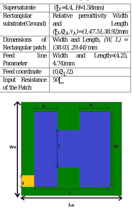
The objective is to design a single band microstrip patch antenna for wireless communication resonance at 2.4Ghz. the substrate material is chosen as a RT Duriod with permittivity 4.4 and loss tangent as 0.0013 with substrate height 1.58mm. the substrate dimension 38.92*47.51*1.58 mm3 (La*Wa*h). for this antenna we have taken length of the patch (L) is 29.44mm and width (W) is 38.03mm mounted on the substrate. The microstrip feed line with length is 4.74mm and width is 4.25 mm have been used for this antenna. Dimension describe in table 1 and geometry of H shape antenna show in fig 1.

A. Design Procedure

1) Determinethe width of the microstrip patch antenna by equation(1)

2) =

(Є )/ (1)

Determine effective dielectric constant, Ɛreff, using equation (2)

Ɛreff=(Ɛ )+(Ɛ )[1 + 12 ] (2)

3) Calculate the length extension ΔL,by using equation (3)

∆

= 0.412(Ɛ . )( . )

(Ɛ . )( . ) (3)

4) The patch length of the microstrip antenna is calculated by using equation(4) L=

Where the effective length( Leff) of the patch =

√Ɛ (5)

5) dimensions of ground is determine by a= 6h + L

a=6h +W

Table 1: Parameter for H-shape patch antenna

Figure 1: Geometry of Proposed Antenna

III. PARTICLE SWARM OPTIMIZATION TECHNIQUE

Particle swarm optimization (PSO) technique discovered by Eberhart and Kennedy in 1995, it is inspired by social behavior of a swarm of bees, fish and any other animal which is moving in the group. It is based on random probability distribution algorithm[4] when a group of bees in garden, they always try to discover a huge number of flower[5]. This method is used when a large number of particle from a group moving around in search space seeking for a optimized solution [3] . In this technique every particle is supposed as a point in an N- dimensional space, which adjust its flying according to its flying experience as well as its flying experience of other particle[6]. Each particle seek to change its position using the details of current position, the current velocity , the distance between the current position and the personal best position(Pbest), the distance between the current position and global best position (Gbest). The algorithm is formulated by below equation.

Vid = W×Vid – 1 +C×η1×(Pid-1 – Pid-1) +C2×η2×(Pgd - Xid– 1)(6)

Xid=Xid-1 + Vid(7)

Supersaturate ( =4.4, H=1.58mm) Rectangular

substrate(Ground)

Relative permittivity Width

and Length

( , , )=(1,47.51,38.92)mm

Dimensions of Rectangular patch

Width and Length, (W, L) = (38.03, 29.44) mm

Feed line Parameter

Width and Length=(4.25, 4.74)mm

Feed coordinate (0, /2) Input Resistance

of the Patch

Where Vid is the velocity &Pidis the best position of the ith particle, Pgd dimension, Xid is the position, C1 & C2 are position constant,

η1 & η2 are random function in the range (0,1), w is the inertia weight[7]

Produce the initial population is the primary step in PSO Algorithms. The primary evaluation of populations is called the “fitness function”. If the fitness value is large, then performance will be better. After the calculation of the fitness function, the fitness value and maximum number of the iterations are determined to know whether or not the evolution process is completed (Maximum generation number reached)[4-6].

A. Optimization by PSO

The parameter (a,b,c and d) of the antenna is optimized to form the position of the particle. The Fitness of every position is based on the cost function and input provided other parameter(dielectric constant, size of the substrate, substrate thickness). The antenna characteristic has single objective (e.g. only resonant frequency or only bandwidth) or multi objective (both resonance frequency and bandwidth) frequency of antenna taken mutually. The objective of this optimization process was keeping the resonance frequency near to 2.4Ghz and maximize the fractional bandwidth(FBW) by varying the parameter (a, b, c and d).

B. Curve fitting

To generate the relationship between resonance frequency or FWB and parameter of antenna. First one parameter is varied while keeping other parameter constant. table 2 show the range of all parameter

Table 2:range of parameter H-shape antenna

Parameter a is varied from 6mm to 17mm with increment of 1mm same way b, c is varied from initial value to final value with increment of 1mm but d is varied from 0.5mm to 6.5mm with increment of 0.5mm. so total (11+16+28+12+1)68 are obtainable and for every antenna calculated resonance frequency and FBW . Apply this value in the Graphmatica (curve fitting software) and obtained the relationship between parameter (a,b,c, and d) and resonance frequency and FBW two of these given below.

BW1= 0.0006*a^4 - 0.0228*a^3 - 0.0442*a^2 + 6.6337*a - 32.0705 (6) FR1 = 1.0642*10^-5a^4 - 7.8571*10^-5a^3 - 0.0019a^2 + 0.038a + 1.7607 (7)

C. Fitness function

The Root Mean Square Error Ei is used to generate the fitness function. The Root Mean Square ErrorEi is evaluated by below formulas

Ei = ∑ ( − ) (8)

Where Pi j is the rate suppose by the separate program i for fitness case j. Pi j = Tj and Ei = 0 is necessary for perfect fitness. By using above fitness function our fitness formulas is

F(x)= ( − arg ) + ( − arg )

Where,

M and N are the biasing constant of each term and arg , arg are the desired resonance frequency and desired bandwidth.

M is bias to develop PSO optimization for the resonance frequency and N is bias to develop PSO optimization bandwidth FBW[6].. Paramete r Initial value Final value

a 6mm 17mm

b 1mm 17mm

c 9mm 37mm

Table 3: Comparison between Conventional to Optimized Antenna

IV. RESULT AND DISCUSSIONS

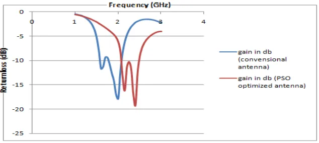
By help of above relationship we wrote a MATLAB program for PSO and RMSE based fitness function and than run it. The value of M and N are fix at 0.40 and 0.60, and iteration 200 with 100 particle. We found the value of four optimized parameter show in the table 3. Design and simulated the optimized antenna with help of ansoft HFSS and than compare with conventional antenna show in fig 2.

Figure 2: Comparison of Return Loss graph

V. CONCLUSION

In this work PSO is used for optimization the parameter of the antenna. After optimization bandwidth increase from 16.10% to 18.22% and antenna resonance at 2.4Ghz frequency. It can be conclude that PSO is fast and accurate optimization technique. In the return loss plot show that antenna resonated exactly at 2.4GHZ so PSO restricted that version from central frequency.

REFERENCES [1] A.BALANIS, Antenna Theory Third Edition, Analysis and Design4

[2] MT Islam, N Misran,T C Take, design Optimization of microstrip patch antenna using particle swarm optimization,Electrical Engineering and Informatics, 2009. ICEEI '09. on International Conference

[3] A Das, MN Mohanty and R K Mishra, optimized design for H slot antenna for bandwidth improvement ,power communication and information technology conference 2015 IEEE

[4] Kennedy, J., Eberhart, R.C.: Particle swarm optimization. Proc. IEEE Int. Conf.

[5] Shi Y. and Eberhart. R.C, "A modified particle swarm optimizer, "Proceedings of the IEEE International Conference on Evolutionary Computation. IEEE Press, Piscataway, NJ (1998), pp. 69-73.

[6] ] Vivek Rajpoot, D K Srivastava, optimization of I shape Microstrip Antenna Using PSO And Curve Fitting, Published on 11 Oct.2014 By Springer Science New Yark 2014

[7] Y Choukikar, S K Behera, R K Mishra , optimization of dual band microstrip patch antenna using PSO, IEEE apply electromagnetic conference 2009 [8] Ansoft HFSS study manual, HFSS .13.

[9] ] Gilat, Amos: MATLAB An Introduction with Applications. Wiley,Hoboken, NJ (2008)

Parameter Conventional antenna

PSO Optimized Antenna

a (mm) 11 1.5

b(mm) 13 4.3

c(mm) 16 25

d(mm) 4 5.4

(GHz) 2.00 2.4