Image Denoising using Principal Component Analysis in Wavelet Domain and Total Variation Regularization in Spatial Domain

Image Denoising using Principal Component Analysis in

Wavelet Domain and Total Variation Regularization in

Spatial Domain

Brajesh Kumar Sahu

Samrat Ashok Technological Institute, Vidisha

Preety D. Swami

Department of Electronics & instrumentation Samrat Ashok Technological Institute, Vidisha

ABSTRACT

This paper presents an efficient denoising technique for removal of noise from digital images by combining filtering in both the transform (wavelet) domain and the spatial domain. The noise under consideration is AWGN and is treated as a Gaussian random variable. In this work the Karhunen-Loeve transform (PCA) is applied in wavelet packet domain that spreads the signal energy in to a few principal components, whereas noise is spread over all the transformed coefficients. This permits the application of a suitable shrinkage function on these new coefficients and elimination of noise without blurring the edges. The denoised image obtained by using the above algorithm is processed again in spatial domain by using total variation regularization. This post processing results in further improvement of the denoised results. Experimental results show better performance in terms of PSNR as compared to the performance of the methods when incorporated individually.

Keywords

Image denoising, Principal component analysis, Total variation regularization, Wavelet packet transform.

1. INTRODUCTION

Real world images do not exist without the noise. Principal sources of noise in the digital images arise during image acquisition and transmission. The amount of noise depends on the different factors such as CCD cameras, light levels and sensor temperature. During transmission, images are corrupted mainly due to interference in the channel used for transmission. The mathematical model of noisy image is given by

𝑓 = 𝑓 + 𝜂 (1)

Where 𝑓 is the noisy image, 𝑓 is the original image and 𝜂 is the additive white Gaussian noise with zero mean and standard deviation 𝜎. All denoising methods are a type of low pass filtering. Filtering can be done in the spatial domain or in the transform domain. Filtering in the transform domain is more efficient and introduces fewer artifacts. The traditional linear filtering methods in spatial domain are Wiener filtering and mean filtering, whereas nonlinear filtering can be done through median filtering [1,2]. The drawback of these filtering methods is that they do not preserve the edges in the denoised image. Donoho and Johnstone introduced denoising via wavelet thresholding [3,4,5] and it is now widely applied in science and engineering applications. It is based on thresholding (adaptive or nonadaptive)

of the wavelet coefficients obtained from the orthogonal discrete wavelet transform (DWT) of data. The wavelet coefficients in the frequency detail subbands can be thresholded by means of soft/hard thresholding operator. Another image denoising scheme is by using Principal Component Analysis (PCA) [6,7]. It transforms the original data set in to PCA domain and by preserving only the most significant principal components, the noise and trivial information can be removed. In [8], PCA based method was proposed for image denoising using local pixel grouping. Drawback of this scheme is that due to its computational complexity it is very slow.

The proposed work combines the good properties of wavelet packet analysis with those of principal component analysis, realized using the Karhuen-loeve (KL) transform in wavelet domain. The KL transform in wavelet packet domain fully decorrelate the frequency subbands, wherein the energy of the signal is clustered in few principal components while the noise energy spread over all transformed coefficients. This allows to apply a suitable shrinkage function to these new coefficients, thus removing noise without blurring the edges. The resulting image is processed again in spatial domain by using total variation regularization.

Rest of the paper is organized as follows: Section 2 presents the general theory of wavelet packet decomposition. Section 3 briefly reviews the procedure of PCA. Image denoising using total variation regularization is presented in Section 4. Section 5 is devoted for the description of the proposed algorithm and Section 6 presents the experimental results and comparison. Finally, Section 7 concludes the paper.

2.

WAVELET

PACKET

DECOMPOSITION

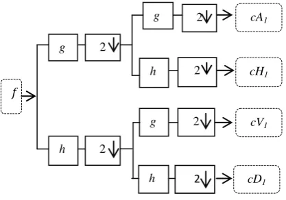
Fig 1: First level wavelet packet decomposition

3. PRINCIPAL COMPONENT ANALYSIS

PCA [6,10,11] is a classical decorrelation technique which is mostly used for data compression, patter recognition and noise reduction. A remarkable property possessed by PCA is that the energy of signal concentrates on a small subset of PCA transformed data set while the noise energy spreads over the whole dataset. Therefore, signal and noise can be distinguished in the PCA transform domain.

Assume z = [𝑧1,𝑧2, 𝑧3… . . 𝑧𝑚 ] to be an m- component vector variable. Z, the 𝑚 × 𝑛 sample matrix of z, is given by

Z =

𝑧11 𝑧12 … 𝑧21 _𝑧22 _… ⋮ ⋮ ⋮

𝑧1𝑛 𝑧2𝑛 ⋮ 𝑧𝑚1 _𝑧𝑚2 _{… 𝑧𝑚}𝑛

(2)

For i = 1, 2, 3 ………m and j = 1, 2, 3 ……n,𝑧_𝑖𝑗 is the discrete sample of variable 𝑧𝑖. The ith row of sample matrix given by Zi = [𝑧_𝑖1 𝑧_𝑖 2 … … . 𝑧_𝑖𝑛], is the sample vector of 𝑧𝑖.The mean value of 𝑧𝑖 is estimated as µ𝑖= 𝐸 𝑧 𝑖 ≈ _𝑛1 𝑛𝑗 =1Zi j . Thus the mean value vector of z is given by

µ = 𝐸[z] = [µ1 µ2 … . . . µm]𝑇 (3)

Centralized vector z = z − µ, and the element of z is𝑧 𝑖= 𝑧𝑖− µ𝑖 . The sample vector of 𝑧 𝑖 isZ i= Zi− µ𝑖= [𝑧 𝑖1𝑧 𝑖2… . 𝑧 𝑖𝑛], where 𝑧 _𝑖𝑗 = 𝑧_𝑖𝑗 − µ𝑖. Accordingly the centralized matrix Z of Z is given by

Z = Z 1 Z 2 ⋮ Z m

=

𝑧 11 𝑧 12 … 𝑧 21 _{𝑧 2}1 _… ⋮ ⋮ ⋮

𝑧 1𝑛 𝑧 2𝑛 ⋮ 𝑧 𝑚1 _{𝑧 𝑚}2 _{… 𝑧 𝑚}𝑛

(4)

The co-variance matrix of Z is calculated as

Ω ≈ (1/n)Z ZT (5)

In PCA transformation, an orthonormal transformation matrix P is calculated to decorrelate Z , i.e. X = PZ such that the co-variance matrix of X is diagonal. The co-variance matrix Ω of Z is symmetrical so it can be written as

Ω = ФᴧФT (6) where, Ф = [ɸ1ɸ2… … … . . ɸ𝑚] is the 𝑚 × 𝑚 orthonormal eigenvector matrix and ᴧ = 𝑑𝑖𝑎𝑔{𝜆1, 𝜆2, … … . , 𝜆𝑚} is the diagonal eigenvalue matrix with 𝜆1≥ 𝜆2… … … … ≥ 𝜆𝑚 . The terms ɸ1, ɸ2, … … … , ɸm and 𝜆1, 𝜆2, … … . , 𝜆𝑚 are the eigenvectors and eigenvalues of Ω respectively. By putting P = ФT (7)

Z can be decorrelated, i.e. X = PZ and ᴧ= (1/n ) X X𝑇 .

4. TOTAL VARIATION

REGULARIZATION

Total variation, also known as the total variation regularization process is based on the principle that the signals with excessive and possible spurious details have high total variation, that is, integral of absolute gradient of the signal is high. By using this principle, upon reducing the total variation of the signal results in a close match to the original signal, thus removing undesired details (noise) while preserving the important details such as edges. For an input image𝑓 the goal of total variation is to estimate𝑓"that has a smaller total variation than 𝑓 (noisy image) but is close to 𝑓 . One measure of closeness is sum of square error.

Total variation denoising problem is of the form proposed in [12].

min_𝑓" 𝑙𝑚₂ 𝑓 − 𝑓" 2+ 𝑣(𝑓") (8)

Where

𝑣 𝑓" = 𝑓𝑖 ,𝑗 _𝑖+1,𝑗" − 𝑓_𝑖,𝑗" 2+ 𝑓_{𝑖,𝑗 +1}" − 𝑓_𝑖,𝑗" 2

(9)

and lm is the regularization parameter, which plays an important role in denoising. If 𝑙𝑚= 0, there is no denoising. Depending upon the noise level, 𝑙𝑚 can have a value between 0 and 1.

5. PROPOSED DENOISING ALGORITHM

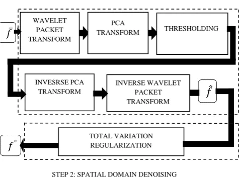
In this section the proposed denoising algorithm is discussed. The original image 𝑓, of size 𝑚 × 𝑚 is corrupted by additive white Gaussian noise (𝜂) with zero mean and standard deviation σ. The noisy image is represented by 𝑓 𝑓 = 𝑓 + 𝜂 . Denoising is performed in two steps; Step 1: Wavelet packet denoising using PCA, Step 2: Post processing of the denoised image of step1 through the Total Variation Regularization in the spatial domain. The block diagram of the proposed technique is shown in Fig. 2.

Step 1: In the first step, the wavelet packet decomposition of noisy image is obtained by using the well-known tensor product technique. The l level decomposition of the noisy image (𝑓 ) of size 𝑚 × 𝑚turns out in to T = 2𝑙× 2𝑙 subband images represented by𝑐𝑗 (𝑗 = 1, 2, … 2𝑙× 2𝑙 ), each of size of 𝑘 = 𝑚/2𝑙_{× 𝑚/2}𝑙_{. Each sub image is arranged in the form of a} singlerow of matrixZ. Thus,2𝑙× 2𝑙 subbands when arranged in the matrix Z, makes the dimension of the matrix to be (2𝑙× 2𝑙_{) × ( 𝑚/2}𝑙_{× 𝑚/2}𝑙_{). Then KL (PCA) transform is applied to} the matrix Z and the transformed matrix is represented by X. The PCA transformed wavelet packet coefficients are represented by 𝑐 𝑗 ,𝑘. The KL transform separates the signal and 𝑓

cA1

cH1

cV1

cD1 2

g

2 h 2

g

2

2 g

h 2

noise energy, thus allowing to apply a new thresholding rule as proposed in [13]. All the frequency sub bands whose mean energy is less than the Gaussian noise variance (𝜎2) are discarded and an exponential shrinkage function as proposed in [14] is applied to the retained coefficients.

𝐹𝑡(𝑥) = 𝑎−𝑕 𝑡2

𝑥2if 𝑥 ≠ 0 with

0 otherwise 𝑎 ≥ 1 &𝑕 ≥ 0 (10) The threshold t is band dependent which means that each subband (𝑐𝑗) has an individual threshold depending on the mean energy of subband (i.e., 𝜆𝑗) and is given by 𝑡𝑗 for j =1, 2, 3……. (2𝑙× 2𝑙 ).

𝑡𝑗 = 𝜆𝑗𝜎2

𝜆𝑗−𝜎2 (11)

The thresholded coefficient is given by𝑐 𝑗 ,𝑘 𝑗 = 1, 2, … 2𝑙×

2𝑙 𝑎𝑛𝑑 𝑘=1, 2,…𝑚/2𝑙× 𝑚/2𝑙.

𝑐 𝑗 ,𝑘= 𝐹𝑡𝑗 𝑐 𝑗 ,𝑘 × 𝑐 𝑗 ,𝑘 if 1 k 𝑐 𝑗 𝑐 𝑗 𝑇_{≥ 𝜎}2 0 otherwise (12) Application of inverse PCA and then the inverse wavelet packet transform to the thresholded coefficients results in the denoised image of step 1.

Step 2: In the second step, the resulting denoised image 𝑓 of step 1 is treated as input image for denoising in the spatial domain by using the total variation regularization using Equation (8), and Chambolle‟s minimization algorithm proposed in [15].

STEP 1: WAVELET DOMAIN DENOISING

STEP 2: SPATIAL DOMAIN DENOISING

Fig 2: Block diagram of proposed denoising algorithm.

6. EXPERIMENTAL RESULTS AND

COMPARISON

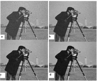
The performance of the proposed denoising algorithm is tested on four gray-scale images shown in Fig. 3, each having a size of 512×512. These test images have been corrupted with Gaussian noise with different values of standard deviation (σ = 5, σ = 10, σ = 15, σ =25, σ =35). In the first step of the proposed

denoising algorithm, 3 level (l=3) wavelet packet decomposition is performed using „sym8‟ wavelet for decomposition instead of „db4‟ used by the authors in [13]. The near symmetry property of „sym8‟ wavelet finds advantage over „db4‟ in image processing applications as symmetry is a desirable property for the human visual system. For exponential shrinkage, a possible choice for the parameters h and a is h=4 and a=2 (generally these values depend on the amount of noise). In the second step of denoising, the denoised images obtained from the first step are further processed with TV regularization with differing values of regularization parameter 𝑙𝑚. Each image with standard deviation of noise (σ = 35, 25, 15, 10, 5) were tested for all possible values of 𝑙𝑚ranging from 0.1 to 0.9. Experiments show that, higher value of 𝑙𝑚 is required for post-processing of images that were suffering from low noise levels and vice-versa. TV regularization parameter taken is 𝑙𝑚= 0.1, 0.2, 0.5, 0.7, 0.9 for the noise deviation σ = 35, 25, 15, 10, 5 respectively. Table 1 shows the experimental results in terms of root mean square error (RMSE) and peak signal to noise ratio (𝑃𝑆𝑁𝑅 = 20 log10(255/RMSE)). Table 2 shows the comparison of denoised results of proposed method with the soft thresholding (using the universal threshold) method, TV regularization method and PCA in wavelet domain method in terms of RMSE and PSNR. It is very clear from the comparative table that only for the low noise deviation (σ = 5) , PSNR of denoised Lena image of proposed method is low as compared to TV regularization method while for higher noise deviations, it is the highest as compared to all the methods under comparison. The PSNR of denoised cameraman and MRI image of proposed method for all noise deviations is high as compared to all the methods under comparison. For the denoised peppers image of proposed method, the PSNR is low as compared to TV regularization method for low noise deviation (σ = 5, σ = 10, σ = 15), but for higher noise deviations (σ = 25, σ = 35), the proposed method provide the best results. Denoised images of Lena, Cameraman, MRI, and Pepper by using different methods (TV regularization, PCA in wavelet domain, and proposed method) are shown in Fig. 4, Fig. 5, Fig. 6 and Fig. 7 respectively.

Fig3: Test images (a) Lena; (b) Cameraman; (c) MRI; (d) Peppers

𝑓

𝑓

𝑓"

THRESHOLDING PCA

TRANSFORM WAVELET

PACKET TRANSFORM TRANSFORM

INVERSE WAVELET PACKET TRANSFORM INVESRSE PCA

TRANSFORM

TOTAL VARIATION REGULARIZATION

a

_b

Table 1. Numerical results on the test images with several noise standard deviation values.

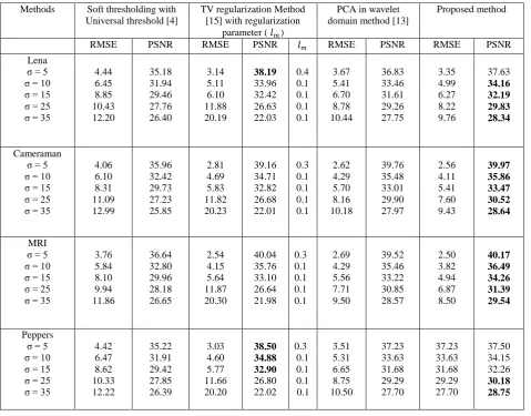
Table 2. Comparison between the soft thresholding with universal threshold method [4], TV regularization method [15], PCA in wavelet domain method [13], and proposed method in terms of RMSE and PSNR.

Noise deviation (σ) and TV regularization parameter (lm)

Lena Cameraman MRI Peppers

RMSE PSNR RMSE PSNR RMSE PSNR RMSE PSNR

σ = 5 lm = 0.9 3.35 37.63 2.56 39.97 2.50 40.17 3.40 37.50 σ = 10 lm = 0.7 4.99 34.16 4.11 35.86 3.82 36.49 5.00 34.15 σ = 15 lm = 0.5 6.27 32.19 5.41 33.47 4.94 34.26 6.22 32.26 σ = 25 lm = 0.2 8.22 29.83 7.60 30.52 6.87 31.39 7.90 30.18 σ = 35 lm = 0.1 9.76 28.34 9.43 28.64 8.50 29.54 9.31 28.75

Methods Soft thresholding with Universal threshold [4]

TV regularization Method [15] with regularization

parameter ( 𝑙𝑚)

PCA in wavelet domain method [13]

Proposed method

RMSE PSNR RMSE PSNR 𝑙𝑚 RMSE PSNR RMSE PSNR

Lena σ = 5 σ = 10 σ = 15 σ = 25 σ = 35

4.44 6.45 8.85 10.43 12.20 35.18 31.94 29.46 27.76 26.40 3.14 5.11 6.10 11.88 20.19 38.19 33.96 32.42 26.63 22.03 0.4 0.1 0.1 0.1 0.1 3.67 5.41 6.70 8.78 10.44 36.83 33.46 31.61 29.26 27.75 3.35 4.99 6.27 8.22 9.76 37.63 34.16 32.19 29.83 28.34 Cameraman σ = 5 σ = 10 σ = 15 σ = 25 σ = 35

4.06 6.10 8.31 11.09 12.99 35.96 32.42 29.73 27.23 25.85 2.81 4.69 5.83 11.82 20.23 39.16 34.71 32.82 26.68 22.01 0.3 0.1 0.1 0.1 0.1 2.62 4.29 5.70 8.16 10.18 39.76 35.48 33.01 29.90 27.97 2.56 4.11 5.41 7.60 9.43 39.97 35.86 33.47 30.52 28.64 MRI σ = 5 σ = 10 σ = 15 σ = 25 σ = 35

3.76 5.84 8.10 9.94 11.86 36.64 32.80 29.96 28.18 26.65 2.54 4.15 5.64 11.87 20.30 40.04 35.76 33.10 26.64 21.98 0.3 0.1 0.1 0.1 0.1 2.69 4.29 5.56 7.71 9.50 39.52 35.46 33.22 30.85 28.57 2.50 3.82 4.94 6.87 8.50 40.17 36.49 34.26 31.39 29.54 Peppers σ = 5 σ = 10 σ = 15 σ = 25 σ = 35

Fig 4: (a) Lena noisy image with σ = 25; (b) denoised image with TV regularization algorithm, PSNR=26.63; (c) denoised image with PCA in wavelet domain, PSNR=29.26; (d) denoised image with proposed algorithm, PSNR=29.83.

Fig 5: (a) Cameraman noisy image with σ = 25; (b) denoised image with TV regularization algorithm, PSNR=26.68; (c) denoised image with PCA in wavelet domain, PSNR=29.90; (d) denoised image with proposed algorithm, PSNR=30.52.

a b

c d

a b

Fig 6: (a) MRI noisy image with σ = 25; (b) denoised image with TV regularization algorithm, PSNR=26.64; (c) denoised image with PCA in wavelet domain, PSNR=30.85; (d) denoised image with proposed algorithm, PSNR=31.39.

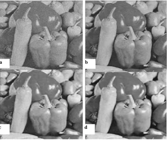
Fig 7: (a) Peppers noisy image with σ = 25; (b) denoised image with TV regularization algorithm, PSNR=26.80; (c) denoised image with PCA in wavelet domain, PSNR=29.29; (d) denoised image with proposed algorithm, PSNR=30.18.

h

d c

a b

c d

7. CONCLUSION

This paper presents a denoising algorithm which is a combination of denoising in both the wavelet domain and the spatial domain. The first stage of denoising is performed by applying PCA on the wavelet packet transform coefficients. PCA owns the property of decorrelation and thus energy of signal concentrates on a small subset of PCA transformed data set while the noise energy spreads over the whole dataset. By applying a suitable shrinkage function, signal and noise are separated in the PCA domain. The second stage of denoising is a post processing step performed in spatial domain using total variation regularization. Experimental results demonstrated that the proposed method can effectively suppress the noise and at the same time effectively preserve the edges without blurring.

8. REFERENCES

[1] S. Jayaraman, S. Esakkirajan, and T. Veerakumar, Digital image processing, McGraw Hill, India, 2012.

[2] S. Dangeti, “Denoising technique comparison,” M Tech thesis, Andhra University college of Engineering, Visakhapatnam, India, 2000.

[3] D. L. Donoho and I. M. Johnstone, “Ideal spatial adaptation via a wavelet shrinkage,” Biometrica, vol. 81, pp. 425-455, 1994.

[4] D. L. Donoho, “De-noising by soft-thresholding,” IEEE Trans. on Information Theory, Vol. 41, pp. 613-627, 1955. [5] D. L. Donoho and I. M. Johnstone, “Adapting to unknown

smoothness via Wavelet shrinkage,” Journal of American Statistical Association, Vol. 90, pp. 1200-1224, 1995. [6] D. D. Muresan, T.W. Parks, “Adaptive principal

components and image denoising,” International

Conference on Image Processing, Vol. 1, pp. 1101-1104, 2003.

[7] Y. Zu, Lecture notes on “Machine learning: Principal component analysis,” 10-701, Spring 2012.

[8] L. Zhang, W. Dong, and D. Zhang, “Two stage image denoising by principal component analysis with local pixel grouping,” Pattern Recognition, Vol. 43, pp. 1531-1549, 2010.

[9] R. C. Gonzalez, and R. E. Woods, Digital image processing, Pearson Education, india, 2010.

[10] A. Ghodsi, Dimensionality reduction a short tutorial, Department of statistics and actuarial science, University of Waterloo, Canada, 2006.

[11] A. Farag, and S. Elhabian, A tutorial on principal component analysis, University of Louisville, CVIP lab, 2009.

[12] L.I. Rudin, S. Osher, and E. Fatemi, “Nonlinear total variation based noise removal algorithm,” Physican D,Vol. 60, pp. 258-268, 1992.

[13] S. Bacchelli, and S. Papi, “Image denoising using principal component analysis in the wavelet domain,” Journal of Computational and Applied Mathematics, Vol. 189, pp. 606-621, 2006.

[14] S. Bacchelli, and S. Papi, “Filtered wavelet thresholding methods,” Journal of Computational and Applied Mathematics, Vol. 164-165, pp. 39-52, 2004.

[15] A. Chambolle, “An algorithm for total variation minimization and applications,” Journal of Mathematical Imaging and Vision, Vol. 20, pp. 89-97, 2004.