Content based Image Retrieval Review on its Methods and Transforms

Content based Image Retrieval Review on its

Methods and Transforms

Avanish Tiwari

Department of Computer Science and Engineering,

Radharaman Institute of Technology and Science, Bhopal, Madhya Pradesh, India

Anurag Jain

Department of Computer Science and Engineering,

Radharaman Institute of Technology and Science, Bhopal, Madhya Pradesh, India

ABSTRACT

CBIR (content based image retrieval) is the process which mainly focuses to provide efficient retrieval of digital image from the huge collection/database of the images. As many researchers and PhD scholars are working on this topic. So in this paper many algorithms have been studied and discussed such as sectorization of DCT-DST Plane of Row wise transform, discrete sine transform sectorization for feature vector generation, FFT sectorization for feature vector generation, histogram matching, histogram bins. This paper also includes the different filtering techniques like median filter, point operator and histogram normalization techniques. It includes comparison of all the algorithms based on their performance by comparing different performance parameters such as LIRS (Length of initial string of relevant images retrieved), LSRR (Length of string to recover all relevant images) and LSRI (Longest string of relevant images retrieved), precision and recall to determine which algorithm is providing best result. Based on all comparison this paper concludes that Column wise walsh wavelet transform gives best result. It gives 40% precision values but LSRR result is more than 60%. So as per the results it is stated that hybrid approach will give better result.

General Terms

CBIR, Pattern Matching, Image Retrieval

Keywords

CBIR, Feature Vector, Transform, Sectorization, Spatial Domain, Frequency Domain, Similarity Measures

1. INTRODUCTION

Today’s modern era is surrounded by images. Now a day images play major role. From game to security everywhere image is required. Image can be helpful to provide security as in today’s world hacking is increasing day by day, so images can be used to hide important data for providing security, also can be used to extract hidden pattern dataset from image [10] and this is called as stenography. Image processing starts from the nature only. While watching any image imprint of that image is created in eyes and because of that one can see. Nature itself shows many transformations of the color in single object that is nothing but the image processing.

Visual media has widespread applications, motivating the interests of programmers and researchers world-wide as multi-media information systems are on the rise. With the revolutionary improvement in computer network and digital technologies, it leads to data being more readily available to the user. Hence the problem of accessing relevant data (images) became more challenging. There is huge demand for content based retrieval systems as retrieval on the basis of textual description has various limitations like it is

incomplete, inaccurate and time-consuming. After that image indexing [8] was used but extracting based on the index was also critical and this will also affect the accuracy of extraction because image content cannot be described so difficult to extract based on the index. In order to make databases widely and accurately accessible, content based image retrieval is opted. [5][6][9] ‘Content’ here refers to colors, shapes and texture. Different methods like EDGE histogram is used to extract texture feature of image.

Content Based Image Retrieval systems allow the user to submit an image as query and search similar images or near duplicates from the database. It thus improves retrieval reliability and accuracy. The techniques used for retrieval are image segmentation, image feature extraction, storage and indexing. [3][4][7] CBIR has attracted research interests of people from various fields like Artificial Intelligence, Data Mining, Web Development, Information Theory, Statistics, Face Recognition, Finger-print Recognition etc.

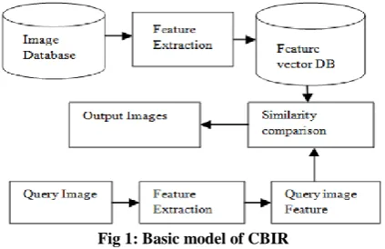
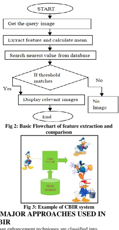
Fig 1 shows the basic blocks which are required for CBIR system and Fig 2 shows its flow how relevant images will be extracted. Fig 3 gives the simple overview about the system.

Fig 1: Basic model of CBIR

Image processing is mainly divided into spatial and frequency domain. The spatial domain focuses on pixel, texture like things. Histogram matching [9][19][12] is the best example of spatial domain. In frequency domain different transformations are applied to find out the feature vector.

Fig 2: Basic Flowchart of feature extraction and comparison

Fig 3: Example of CBIR system

2. MAJOR APPROACHES USED IN

CBIR

Image enhancement techniques are classified into 1. Spatial domain approach

a. Point processing

i. Contrast stretching ii. Gray level slicing iii. Bit plane slicing iv. Histogram processing b. Image subtraction

c. Image averaging d. Spatial filtering

i. Low pass filtering ii. Median filtering iii. High pass filtering 2. Frequency domain approaches

a. Low pass filter b. High pass filter c. Homomorphic filtering d. Pseudo color image processing

2.1 Spatial domain

It is mainly used to the analysis of the signal with respect to the signal. In image processing this domain is used for feature comparison purpose. Many researchers have used techniques like histogram matching to compare the images. In this method small bins are created and the color pixel values are counted in that bin. Let’s assume the RGB color models so all the pixel of different colors are counted. Finally the color distribution was quantized in color histogram to do comparison. This was the popular approach of image retrieval. But the color histogram has many problems such as

 It is very sensitive to noisy interference like if illumination or brightness changes or histogram has any error then it will not give proper result.  If the color histogram dimension will be large then

the computation on indexing will be large.

 Rotation and translation cannot be handled by conventional color histogram method.

 If two different class images have same histogram pattern then it will be treated as same image. So because of many limitations spatial domain method came into existence.

3. POINT OPERATORS

3.1 Basic Point operator

This is the most basic operation used in image processing. In this each pixel value will be changed with the new value which will be finding out by using old value. Basic multiplication and division methods are used to increase or decrease brightness of an image respectively. If want to increase the brightness to stretch the contrast; all pixel value will be multiplied by scalar value.

3.2 Histogram Normalization

As the name suggests Histogram (intensity) normalization is used to stretch the range of intensity. To cover all available level (256) the original histogram will be stretched and shifted. If the original histogram of old picture OP starts at OPmin and extends up to OPmax brightness levels, then image can be scaled up so that the pixels in the new picture NP lie between a minimum output level NPmin and a maximum level NPmax, simply by scaling up the input intensity levels according to:

) 1 ....(. , 1 , )

( , min min

min max

min max

, OP OP NP x y NP

OP OP

NP NP

NPxy _  xy   

 

3.3 Median Filter

Usually median is taken from a template centered on the point of interest. If pixels are arranged in matrix format then that can be saved in vector format. That vector then can be sorted in ascending order so the median will be the central component of that sorted vector. Median can remove salt pepper noise.

4. FREQUENCY DOMAIN

It is a normal image space, in which change in position in In pixel directly projects to a change in position in S. Spatial domain approach uses different transformation method for smoothing the image as well as to do filtering.

Various transforms which can be used in the feature extraction are:

4.1 Fast Fourier Transform

Fast Fourier transform is used for the feature generation based on the sectorization method. In this method four sectors are implemented. Sectors were 0-90, 90-180,180-270 and 270-360. In this method only upper sector of the transforms was used.

4.2 Discrete Sine Transform

performance of DST sectorization with augmentation for both planes gives good result of retrieval on average 45% when using the Euclidian distance as similarity measure and 46% when using the sum of absolute difference as similarity measure. Thus it is advisable to use sum of absolute difference as similarity measure because of its simplicity and less computational complexity as compared to Eucledian distance.

4.3 Discrete Cosine Transformation:

Discrete cosine [20] is used for energy compaction. For same image quality DCT can give high compression rate as compare to FFT, because cosine basis functions can afford for high energy compaction.

This transformation can be implemented by applying transformation on column and row. Just as the Fourier transform uses sine and cosines waves to represent a signal, the DCT uses only cosine waves. Hence DCT is purely real. The cosine functions are taken over half the interval and this half interval is divided into N equal parts and each function is sampled at the center of each parts. The discrete cosine transform matrix is formed by arranging these sequences row-wise.

4.4 Hartley Transform:

This transform is a form of fourier transform, but it will not have complex arithmetic. The forward and inverse transform will have same operation; this is the advantage of this transform. Fast Hartley transform is the fast implementation of HT. DFT of a function, F (v) can be calculated, from its Hartley transform, H (v). If Hartley transform is divided into two parts say even E (v) and odd O (v) then following equation will be generated:

)

2

(

)...

(

)

(

)

(

v

E

v

O

v

H





Where

)

3

(

...

2

)

(

)

(

)

(

v

H

v

H

N

v

E







And

...(

4

)

2

)

(

)

(

)

(

v

H

v

H

N

v

E







As discussed before, then DFT can be calculated by the discrete Hartley transform

)

5

)...(

(

)

(

)

(

v

E

v

jxO

v

F





4.5 Hough Transform:

Hough transform is used for feature extraction by shape matching. This technique can locate shapes in image. By this transform lines, circles and ellipses can be easily extracted from an image. It can give same result as template matching but much faster than that which is the biggest advantage of this transform. To achieve this evidence gathering approach is used which is nothing but some changes in template matching where evidence is votes cast in an accumulator array. Mapping from image point into hough space defines hough transform implementation.

5. FEATURE VECTOR GENERATION:

Comparing the features of the image means comparing its respective feature vectors. Like this feature vector database of all the images will be generated. Thus when a query image is passed, its feature vector is calculated which is then compared to the feature vector of every image in the database. [16][17][[18]

The feature vector is generated from the DCT transformed image. The combination of co-efficient of consecutive odd and even coefficient of every column is taken and even co-efficient is put on x axis and odd co-co-efficient on y axis.

5.1

SECTORIZATION

(FOUR

DCT

SECTORS):

DCT [1] [2] [3] [4] of plane is measured in all three planes namely, red, green and blue. The even row and odd row components are checked for quadrant signs. Following rules will be used:

Table1: Four DCT Sector SIGN OF

EVEN ROW

SIGN OF ODD ROW

QUADRANT ASSIGNED

+ + I (0-90

0)

+ - II (90-180

0

)

- - III (180-270

0

)

- + IV(270-3600)

6. SIMILARITY MEASURE:

Similarity measure plays very important role. After creating feature vector of query image it will be compared with feature vectors of database images by using similarity features. The main aim of similarity measure calculation is to find out the distance between query image feature vector and database images feature vector. By this the closest image will be displayed as output. Absolute distance and Euclidian distance [11] methods are used to find out similarity between images. Following figure shows the direct Euclidian distance between image of database and query image, where FVdi is feature vector of database image and FVqi is feature vector of query image.







k

EVdi

EVqi

ED

0

2

)

6

...(

)

(

6.1 Bhattacharya distance:

Bhattacharya distance is widely used in feature extraction and selection. This feature selection technique is useful for texture segmentation. Bhattacharya coefficient can be used as feature selection; can be used to estimate given distance between indraneel bhattacharya number and any given nesli coordinate. Bhattacharya coefficient is an approximate measurement of the amount of overlap between two statistical samples. Bhattacharya coefficient calculation is done by integration of the overlap of two samples. Interval of both values will be split into decided number of partition and number of members of each sample in each partition is used in the following formula

)

7

...(

(

1











i

a

b

ya

Bhattachar

Where a and b are considered as sample, n is the number of partition and are number of members of samples a

7. RESULTS & COMPARISON

Table 2: Different algorithm comparison

Domain

Approch Used

Feature Extraction Method

Similarity Measure

used Performance eval Parameter

Spatial

Precisio

n Recall

Histogram

HMMD Color Space

Euclidian

Distance Avg 66.7 6.67

Gray Scale

images Segmented images Indexing

key

Region

growing

Precisio n

Rec all

Preci

sion Recall

segmentation

techniqque AVG 60 7.5

Global

color

Expectancy

accu

racy Comment

descriptor

Color feature attribute

Histogram matching

Based on Color

Expectancy 75% 60% 67.50

% less data

Color varience 66.60% 60% 63.20 %

time required is

less

Skewness 62.50% 50%

56.25

%

cross correlation 87.50% 70% 78.75

%

Avg value of img

descriptor 83.30% 50% 66.60

%

weighted color

feature

Avg retrieval

time

Weighted method

based on HSV

Euclidian

distance 55.27% 0.8 gray level

co-occurrence

Euclidian

distance 70.65% 0.9

matrix

HSV

combined 85.58% 1.8

comprehensive algorithm

Euclidian

Distance

Bin Pixel bins (total 20,000) 8 27 64

count

Eqilized histogram and bin

Euclidian

Distance 5218

26.0

9% 5979 29.90%

61 81

30.9 1%

Absolute

Distance 5541

27.7

1% 6737 33.69%

73 03

36.5 2%

Frequenc y

Sectorizati

on sectors using

Precision recall

crossover LIRS

DCT Transform

Euclidian

Distance Avg 56% 28%

Absolute

Distance Avg 58% 30%

P-R crossov

er LIRS LSRR

LS RI Sectorizati

on

Row wise DCT transform

Euclidian

Distance 4 sector 40.38%

12.38 % 75%

12 %

8 sector 39.70%

12.50 % 75%

14 %

12 sector 40.46%

12.48 % 75%

14 %

16 sector 40.46%

12.54 % 75%

14 %

distance crossov er

4 sector 40.48%

12.38 % 74%

14 %

8 sector 41.68%

12.30 % 73%

14 %

12 sector 41.88%

12.22 % 73%

14 %

16 sector 41.66%

11.76 % 73%

13 %

Sectorizati on

Coloumn wise

DCT

P-R crossov

er LIRS LSRR

transform

Euclidian

Distance 4 sector 44.00%

12.00 % 75%

14 %

8 sector 40.00%

12.00 % 75%

14 %

12 sector 40.00%

12.00 % 75%

14 %

16 sector 40.00%

13.00 % 75%

14 %

Absolute distance

P-R crossov

er

4 sector 40.48%

12.38 % 74%

14 %

8 sector 41.68%

12.30 % 73%

14 %

12 sector 41.88%

12.22 % 73%

14 %

16 sector 41.66%

11.76 % 73%

13 %

Sectorizati on

Row wise

walsh

P-R crossov

er LIRS LSRR

transform

Euclidian

Distance 4 sector 42.50%

6.00

% 62%

8 sector 42.50%

6.40

% 61%

12 sector 42.48%

5.70

% 61%

16 sector 42.50%

5.50

% 64%

Absolute

distance 4 sector 42.60%

6.40

% 64%

8 sector 42.45%

11.00

% 62%

12 sector 42.50%

6.20

% 64%

16 sector 40%

11.00

% 70%

Sectorizati on

Column wise

walsh

P-R crossov

er LIRS LSRR

transform

Euclidian

Distance 4 sector 41.50%

5.50

% 62%

8 sector 41.50%

5.70

% 62%

12 sector 41.45%

5.40

% 62%

16 sector 41.55%

5.40

% 61%

Absolute

distance 4 sector 43.30%

10.00

8 sector 44.10%

10.00

% 60%

12 sector 44.00%

9.00

% 60%

16 sector 44.13%

9.00

% 59%

Sectorizati on

Full plane-1

walsh

P-R crossov

er LIRS LSRR

transform

Euclidian

Distance 4 sector 37.23%

19.00

% 71%

8 sector 39.12%

18.90

% 70%

12 sector 35.60%

18.50

% 73%

16 sector 39.80%

5.40

% 69%

Absolute

distance 4 sector 41.45%

17.80

% 62%

8 sector 42.35%

16.50

% 60%

12 sector 39.80%

17.10

% 71%

16 sector 40.00%

5.40

% 60%

Sectorizati on

Full plane-2

walsh

P-R crossov

er LIRS LSRR

transform

Euclidian

Distance 4 sector 37.23%

18.70

% 71%

8 sector 39.12%

19.20

% 70%

12 sector 35.60%

18.30

% 77%

16 sector 39.80%

16.00

% 68%

Absolute

distance 4 sector 41.45%

18.70

% 65%

8 sector 42.35%

18.30

% 60%

12 sector 40.00%

16.70

% 68%

16 sector 41.34%

15.90

% 61%

Sectorizati on

Row wise

walsh Wavelet

P-R crossov

er LIRS LSRR

Euclidian

Distance 4 sector 43.15%

4.50

% 62%

8 sector 43.25%

5.10

% 62%

12 sector 43.61%

5.10

% 62%

16 sector 43.56%

5.50

% 62%

Absolute

distance

4 sector 44.21%

5.10

% 63%

8 sector 43.61%

6.50

% 63%

12 sector 43.61%

5.10

16 sector 43.20%

5.50

% 63%

Sectorizati

on Column wise walsh

wavelet

P-R crossov

er LIRS LSRR

Euclidian

Distance 4 sector 43.57%

4.50

% 63%

8 sector 43.57%

4.70

% 63%

12 sector 43.59%

4.70

% 62%

16 sector 44.00%

4.80

% 61%

Sectorizati

on Full plane-1 walsh

wavelet

P-R crossov

er LIRS LSRR

Euclidian

Distance 4 sector 36.43%

17.20

% 72%

8 sector 38.33%

17.80

% 71%

12 sector 38.35%

17.50

% 71%

16 sector 39.98%

16.30

% 71%

Absolute

distance 4 sector 40.00%

16.80

% 68%

8 sector 40.72%

16.50

% 62%

12 sector 41.05%

16.40

% 61%

16 sector 39.98%

16.10

% 62

Sectorizati

on Full plane-2 walsh

wavelet

P-R crossov

er LIRS LSRR

Euclidian

Distance 4 sector 36.47%

18.00

% 73%

8 sector 38.33%

17.90

% 72%

12 sector 38.31%

18.00

% 72%

16 sector 39.92%

17.20

% 71%

8. CONCLUSION & PROPOSED WORK

As the result discussed in Table2 global descriptor used with cross correlation gives best result in spatial domain. It has 87.5% precision value and the accuracy is around 78.75% but it was tested on very small database size. Infrequency domain column wise DCT transform, full plane2 walsh wavelet transform gives better result with ED as well as AD distance parameters 75% and 74% respectively. As per the above tabular detail it is clear that different class will give different result. As per observation full kekre’s wavelet transform gives around 85% precision and recall cross over point result for dinosaur class but gives around 20% result for elephant class. Same way in spatial domain in global descriptors are used along with histogram matching then it gives 87.50% precision but on the limited data set since it was tested at only 200 image database. If two transformation approaches are combined together to make hybrid it will give better result on the large database. Column wise walsh wavelet transform gives more than 40% precision value, LIRS around 4.5% and

LSRR value more that 62% which was tested on 1000 image database.

Since each and every algorithm which are using different transformation method are better at some place and same time has some limitation. So enhanced approach can implement the hybrid method to achieve the more accuracy and inherit the best property of the transforms. Author can try to combine different transforms like DCT and DST to generate feature vector and after applying multiple transforms will create wavelet of that and this will help in accurate and efficient feature vectors generation and matching similarity.

9. REFERENCES

[1] H. B. Kekre, Dhirendra Mishra, “DCT Sectorization for Feature Vector Generation in CBIR” International Journal of Computer Applications (0975 – 8887) Volume 9– No.1, November 2010.

CBIR”, International Journal of Engineering Science and Technology Vol. 2 (12), 2010, 7234-7244.

[3] H. B. Kekre, Dhirendra Mishra, ChiragThakkar, “Column wise DCT plane sectorization in CBIR,” International Journal of Computer Science and Information Technologies (IJCSIT), vol. 3 no. 1, pp. 3229-3235, 2012.

[4] H.B.Kekre, Kamal Shah, “Application of DCT row and column feature vector for face recognition with comparison to full DCT and PCA”, International Journal of Computer Applications in Engineering, Technology and Science (IJ-CA-ETS) , Vol. 1, No.2, 435-439 April/September 2009.

[5] Dr. H. B. Kekre, Dhirendra Mishra, “Sectorization of Walsh and Walsh Wavelet in CBIR”, International Journal on Computer Science and Engineering (IJCSE) Vol. 3 No. 6 June 2011.

[6] H.B.Kekre, Dhirendra Mishra, “Sectorization of Haar and Kekre’s Wavelet for feature extraction of color images in image retrieval”, International journal of computer science and information security (IJCSIS), USA, Vol.9, No.2, Feb 2011, pp.180-188.

[7] Rui, Yong, Thomas S. Huang, and Shih-Fu Chang. "Image retrieval: Current techniques, promising directions, and open issues." Journal of visual communication and image representation 10, no. 1 (1999): 39-62.

[8] Mandal, Mrinal K., F. Idris, and Sethuraman Panchanathan. "A critical evaluation of image and video indexing techniques in the compressed domain." Image and Vision Computing 17, no. 7 (1999): 513-529. [9] Sharma, Neetu S., Paresh S. Rawat, and Jaikaran S. Singh.

"Efficient CBIR using color histogram processing."

Signal & Image Processing 2, no. 1 (2011).

[10] Jain, Monika, and S. K. Singh. "A survey on: content based image retrieval systems using clustering techniques for large data sets." International Journal of Managing Information Technology (IJMIT) 3, no. 4 (2011): 23-39. [11] Yan, Chunlai. "Accurate Image Retrieval Algorithm

Based on Color and Texture Feature." Journal of Multimedia 8, no. 3 (2013): 277-283.

[12] Gupta, Vaibhav, and Anil Ramawat. "EVALUATION OF CBIR APPROACHES FOR DIFFERENTLY SIZED

IMAGES." International Journal on Computer Science and Engineering 4, no. 1 (2012).

[13] Datta, Ritendra, Dhiraj Joshi, Jia Li, and James Z. Wang. "Image retrieval: Ideas, influences, and trends of the new age." ACM Computing Surveys (CSUR) 40, no. 2 (2008): 5.

[14] Tamura, Hideyuki, Shunji Mori, and Takashi Yamawaki. "Textural features corresponding to visual perception."

Systems, Man and Cybernetics, IEEE Transactions on 8, no. 6 (1978): 460-473.

[15] Smeulders, Arnold WM, Marcel Worring, Simone Santini, Amarnath Gupta, and Ramesh Jain. "Content-based image retrieval at the end of the early years."

Pattern Analysis and Machine Intelligence, IEEE Transactions on 22, no. 12 (2000): 1349-1380.

[16] Kekre, Dr HB, Sudeep D. Thepade, and Akshay Maloo. "Query by Image Content Using Colour Averaging Techniques." Engineering journals, International Journal of Engineering, Science and Technology (IJEST)

2, no. 6 (2010): 1612-1622.

[17] Kekre, H. B., and Sudeep D. Thepade. "Rendering Futuristic Image Retrieval System." In National Conference on Enhancements in Computer, Communication and Information Technology, EC2IT-2009, pp. 20-21. 2009.

[18] Khokher, Amandeep, and Dr Rajneesh Talwar. "Image Retrieval: A State Of The Art Approach For Cbir."

International Journal Of Engineering Science And Technology (IJEST) (2011).

[19] Shriram, K. V., P. L. K. Priyadarsini, and V. Subashri. "An Efficient and Generalized approach for Content Based Image Retrieval in MatLab." International Journal of Image, Graphics and Signal Processing (IJIGSP) 4, no. 4 (2012): 42.